Parametric study and dynamic response analysis of three single curved discrete pontoon floating bridges

ABSTRACT

In this paper, three curved floating bridge concepts with a uniform span of 500 m and different radii of curvature are proposed for the crossing of the coastal waters in Singapore. The bridge girder is supported by 4 pontoons along the bridge length and the two ends are connected to the shore. Three different girder cross-sections are considered. Static analysis is first carried out considering the bridge's self-weight, water current forces and various tidal conditions. Next, eigen value and regular wave analyses are performed to assess the effect of bridge radius, cross-sectional rigidity and end connection on the bridge behaviour. Based on the results, several bridge configurations are selected for further study. Finally, irregular wave analysis is carried out to investigate the realistic bridge performance under operational and extreme environmental conditions. Conclusions are drawn based on the simulation results. Recommendations on the design parameters for further investigations are made.

KEYWORDS:

• Floating bridge
• curved bridge
• hydroelasticity
• irregular waves
• tidal variation

1. Introduction

To sustain the development of coastal metropolises, it is preferable to explore the possibility of utilising the sea space to accommodate excessive industry and transport facilities (Jiang et al. 2018 2019, 2021a, 2021b; Dai et al. 2018, 2019, 2020b). Several notable sea-crossing bridges have been constructed over the world, such as the King Fahd Causeway (1986, Saudi Arabia), the Great Seto Bridge (1988, Japan), the Hangzhou Bay Bridge (2008, China), etc. However, when the water depth is very deep and/or the seabed is extremely soft at a location where a bridge is needed, conventional piers supporting the bridge superstructure become very difficult to be constructed. Under such situations, floating bridges may be a superior and economical alternative as the self-weight and the vehicle loads can be supported by the natural buoyancy of seawater via the use of pontoons or floaters. Additionally, a floating bridge may be removed and relocated with ease by using tugboats when needed.

There is a long history of floating bridges. The first floating bridge can be dated back to about 480 BC, when two rows of floating bridges were constructed for military usage by laying decks over hundreds of boats placed side by side. The first modern floating steel Galata Bridge was completed in 1912. Since then, several other floating bridges were built globally, including the Lacey V. Murrow Bridge (2020m, 1940, USA), the Evergreen Point Bridge (2350 m, 1963, USA), and the Homer Hadley Bridge (1772m, 1989, USA) which were built on Lake Washington, and the Hood Canal Bridge (2398 m, 1961, USA) in Seattle area, USA. In recent decades, two curved floating bridges, namely the Bergsøysund Bridge (931 m, 1992, Norway) and the Nordhordland Bridge (1614 m, 1994, Norway) were built for the crossing of the fjords in Norway. In 2000, the floating movable Yumemai Bridge (876 m, 2000, Japan) was built in Japan (Watanabe and Utsunomiya 2003; Watanabe et al. 2004b).

There are mainly two types of floating bridges: (1) continuous pontoon bridges like the Lacey V. Murrow Bridge and the Hood Canal Bridge, and (2) discrete pontoon bridges like the Bergsøysund Bridge and the Nordhordland Bridge. Different analysis methods have been developed for studying the responses of these two types of floating bridges. Modal expansion method and direct calculation method (Kashiwagi 2000; Watanabe et al. 2004a) are two key frequency domain analysis methods for continuous pontoon floating bridges, while time domain methods can also be used. Hydroelasticity should be considered (Watanabe et al. 2003; Fu et al. 2005) if the bridge is expected to behave flexibly and especially when the eigen frequencies of the bridge are near the environmental load excitation frequency regions. For discrete pontoon bridges, hydrodynamic properties regarding a single pontoon may be considered individually when the pontoon spacing is large enough. The Finite Element Method (FEM) can be used for the bridge superstructure and other structural components. If the pontoons are close to each other or close to the shore, the hydrodynamic interactions between pontoons and the shore should be taken into consideration (Seif and Inoue 1998). A time domain method to simulate the dynamic behaviours of a three-span suspension bridge with two floating pylons was developed (Xu et al. 2017). A sensitivity-based FEM updating method was proposed and applied to the analysis of the Bergsøysund Bridge (Petersen and Øiseth 2017). Model tests on Bergsøysund Bridge were carried out in the ocean basin at MARINTEK (Now Sintef Ocean) in 1989 and the results were compared with numerical calculations based on potential flow theory. The comparison showed that the potential flow theory is able to produce satisfactory predictions (Løken et al. 1990). Furthermore, the uncertainties associated with employing a coupled SIMO-RIFLEX simulation for a curved floating bridge under wave- and current-induced responses were very recently examined through comparison with available model test results (Viuff et al. 2020). The study also shows that the numerical tool is able to generate reliable and accurate results.

Bridge pontoons provide vertical support to the superstructure, while the horizontal bridge stiffness can be achieved by modifying the geometrical properties of the bridge, or/and by engaging additional mooring systems. The Bergsøysund Bridge (Solland et al. 1993) and the Nordhordland Bridge use curved geometrical designs to achieve the arch effect in the horizontal plane and thus no side-anchored mooring systems are needed. Structural modal property is an important aspect and is affected by several parameters including the bridge cross-sectional properties, bridge end connections, number of pontoons, pontoon designs, and bridge curvatures, etc. The dynamic responses of bridges could be excited by various types of environmental loads. Besides, the responses can be strongly amplified due to resonance. An important issue of the floating bridge designs for the crossing of Norwegian fjords is the inhomogeneous environmental conditions, which imposes challenges to the proper modelling of the environmental loads on the bridge structure (Cheng et al. 2018b, 2018c; Dai et al. 2020a, 2021a, 2021b). The wave inhomogeneity is found to induce different dynamic responses when compared with homogeneous wave conditions. Ship collision is also an important aspect of the design consideration. The damage due to collisions on the pontoon wall and bridge girder has been investigated numerically (Sha et al. 2019; Sha and Amdahl 2019). Design limit states of bridge structures, including the Fatigue Limit States (FLS), Ultimate Limit State (ULS), Service Limit State (SLS) and Accidental Limit State (ALS), define various design criteria under different loading conditions. These design limit states pose challenges to the analysis of floating bridges, but ensure proper service states under operational conditions and survivability under extreme or accidental conditions (Lwin 2000; 16th ISSC COMMITTEE VI.2 2006).

In this paper, curved floating bridges with a short span of 500 m are proposed for dynamic response analysis. These bridges are vertically supported by four discrete pontoons. They have potential applications for the crossing of shallow coastal waters in Singapore with a water depth of up to 30 m. Owing to the dense population and high transportation demand, the bridge girder is designed to carry dual three-lane traffic carriageways. To investigate the geometrical effect on the dynamic properties of floating bridges, three different bridge configurations are considered in this study, namely, a straight bridge, a curved bridge with a radius of 1000 m, and a curved bridge with a radius of 500 m. When compared with existing floating bridges, the proposed bridge designs have some distinct features. Firstly, the floating bridge application for a short span crossing with a shallow water depth due to weak seabed conditions. Secondly, they are designed for the crossing of shallow coastal waters in Singapore. Owing to the coastal shallow water condition, the environmental conditions and hydrodynamic loads are significantly different from those deep water conditions. This study investigates different bridge design options under this unique condition. And thirdly, the bridge girders have relatively high flexural rigidities especially in the transverse direction due to the need to carry wide carriageways, thus the design parameters are expected to be different from existing floating bridges. Through numerical investigations, the technical feasibility of these bridge options is evaluated, with the focus on their structural and hydrodynamic performance. Numerical models of the proposed curved floating bridges are first established and then verified by a theoretical model. Next, parametric studies are carried out to examine the various effects of bridge curvature, cross-sectional properties and end connections on the dynamic responses of the bridges. Based on these studies, further improvement on the design could be proposed in the future.

2. Model description

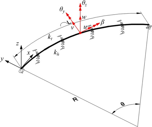
The proposed floating bridges are vertically supported by four identical pontoons. The pontoons have an elliptical cylinder shape with an overall length of 60 m, a width of 22 m and a height of 9 m. The pontoons are treated as rigid bodies with 6 degrees of freedom (D.O.Fs) as shown in Figure 1. The elliptical shape is chosen for the purpose of effectively reducing the current drag forces applied to the pontoon. The three bridge configurations with different radii of curvature are presented in Figure 2. Also shown in this figure are the global coordinate system, local coordinate system, pontoon positions, as well as the geometrical parameters used in the modelling of the bridges. The four pontoons (PT) named PT1, PT2, PT3 and PT4 are evenly distributed along the bridge length, and the pontoon major axis is parallel to the global X-axis. The two ends of the bridge are termed End 1 and End 2. The level of the Center of Gravity (C.O.G) of the pontoon is at −2, and 5 m for that of the bridge girder. The weight of the bridge girder is estimated to be 39.9 ton/m. Note that the stability of the pontoons has been studied previously (Wan et al. 2017b). The dimension and weight parameters of the pontoons and the bridge girder are listed in Table 1.

Figure 1. Elliptic cylinder pontoon supporting the bridge, and the modes of the rigid body motion.

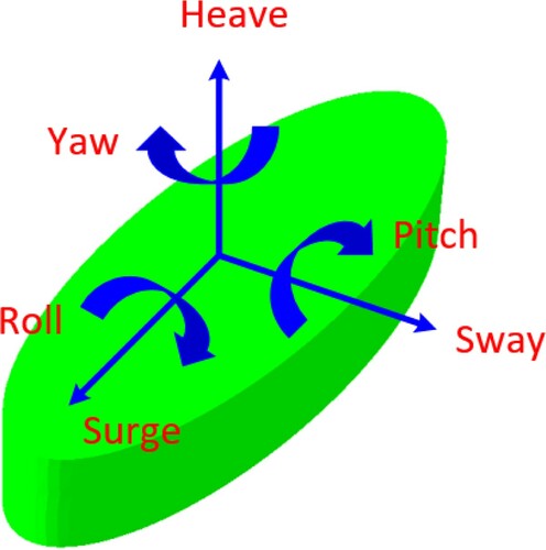
Figure 2. Top view of the three floating bridge configurations with different radii of curvature: (a) straight bridge with infinite radius (RINF); (b) curved bridge with a radius of 1000 m (R1000); and (c) curved bridge with a radius of 500 m (R500).

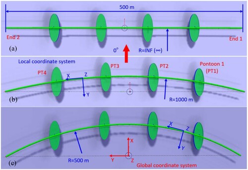
Table 1. Pontoon and bridge girder parameters.

Bridge total length L	500 [m]
Pontoon number	4
Pontoon overall dimension (Elliptic cylinder)	60×22×9 [m]
Pontoon draft	6 [m]
Pontoon C.O.G	(0, 0, −2) [m]
Metacentric height (Horizontal and longitudinal)	3 and 35.5 [m]
Pontoon mass	2319 [ton]
Pontoon rotational inertia Ixx, Iyy and Izz	145,390, 660,290 and 721,030 [ton m^2]
Bridge girder C.O.G	(0,0,5) [m]
Bridge girder weight	39.9 [ton/m]

Floating bridges are intended to be deployed in sheltered coastal areas with benign sea conditions. The operational sea state at the potential site locations with 1-year return period has a significant wave height Hs = 0.88 m and peak period Tp = 5.1 s with a current speed of 1.5 m/s; while the extreme sea state with 100-year return period is: Hs = 2 m, Tp = 5.8 s with a current speed of 1.5 m/s. The daily tide-induced water level variation is ±2 m.

2.1. Numerical model

The hydrodynamic properties of the pontoons, structural properties of the bridge girder and rigidities of the end connections are all taken into consideration. The coupled hydro-structural dynamic model is established. Considering the nonlinear features such as viscous effects and structural geometrical nonlinearities, time domain analysis is carried out. Frequency domain hydrodynamic properties can be pre-calculated by using the Boundary Element Method (Faltinsen 1993) based on the potential flow theory. Then, these properties can be transferred into the time domain for the global analysis considering the bridge structural properties, couplings and external forces. This method may be termed as hybrid time and frequency domain method (Cummins 1962; Naess and Moan 2013), and has been widely employed in various offshore applications (Wu and Moan 1996; Kashiwagi 2004; Karimirad and Moan 2012; Gao et al. 2016; Michailides et al. 2016; Wan et al. 2015, 2016, 2018; Cheng et al. 2018a). In the cases where strongly nonlinear hydrodynamic phenomena are expected, such as slamming or green water problems (Wan et al. 2017a), the linear hydrodynamic model is not suitable anymore, and modifications or nonlinear hydrodynamic models are needed.

The FEM is used for the structural modelling of the bridge girder. The global dynamic equilibrium of the structural finite element formulation in the time domain is expressed as (MARINTEK 2013): (1) $R^I(r,\ddot{r},t)+R^D(r,\dot{r},t)+R^S(r,t)=R^E(r,\dot{r},t)$(1) where $r$, $\dot{r}$ and $\ddot{r}$ are, respectively, the displacement, velocity and acceleration vectors of all the nodes in the FEM model.

$R^I(r,\ddot{r},t)$ is the inertia force vector of the nodes. It includes the inertia of pontoons and the structural mass of the other bridge structural components. The inertia term corresponding to a bridge pontoon can be expressed as $(M+A(\mathrm{\infty })){\ddot{r}}_{PT}^{}(t)$, where $M$ is the mass matrix of the pontoon, $A(\mathrm{\infty })$ is the hydrodynamic added mass matrix at the infinite frequency, and ${\ddot{r}}_{PT}(t)$ is the acceleration vector.

$R^S(r,t)$ is the stiffness force vector, which includes the structural internal stiffness of the bridge structure and the hydrostatic restoring stiffness of the pontoons. Besides, the end connections or boundary conditions of the bridge are also specified in the stiffness force vector.

$R^D(r,\dot{r},t)$ is the damping force vector comprising the structural internal damping and the infinite-frequency wave radiation damping of the pontoons, which is $B(\mathrm{\infty }){\dot{r}}_{PT}^{}(t)$, where ${\dot{r}}_{PT}(t)$ is the velocity of the pontoon. Noted that for floating structures with zero forward speed, $B(\mathrm{\infty })=0$.

$R^E(r,\dot{r},t)$ is the external force vector. This term also includes forces that are not specified in the previous terms. In this study, those forces include the hydrodynamic wave excitation forces, quadratic viscous forces, current forces, tidal variation induced forces, and retardation forces. All these external applied forces are exerted on the pontoons. Note that the quadratic viscous forces are expressed as $C{\dot{r}}_{PT}(t)|{\dot{r}}_{PT}(t)|$, where $C$ is the quadratic viscous damping coefficient matrix, in which the coefficients are set to 0.9 for surge and sway D.O.Fs of the pontoons, 1.2 for the heave D.O.F (DNV 2010). Radiation effects are expressed through the fluid memory effects, or the convolution integral ${\int }_0^{t}k(t-\tau ){\dot{r}}_{PT}(\tau )d\tau$, where $k(\tau )$ is the retardation function matrix, and is expressed as $k(t)={\displaystyle \frac{2}{\pi }{\int }_0^{\mathrm{\infty }}[B(\omega )-B(\mathrm{\infty })]\cos (\omega t)d\omega ={\displaystyle \frac{2}{\pi }{\int }_0^{\mathrm{\infty }}-\omega [A(\omega )-A(\mathrm{\infty })]\sin (\omega t)d\omega ,}}$where A(ω) and B(ω) are, respectively, the hydrodynamic added mass and potential damping at frequency ω. Note that the retardation forces are also applied to the pontoons and are treated as external forces in the finite element model.

In the global finite element model, Euler-Bernoulli beam elements with 6 nodal D.O.Fs (3 translational and 3 rotational) are used to model the bridge girder. The beam cross-sectional properties are specified in terms of the sectional rigidity. The sectional rigidity refers to the axial rigidity EA (in x direction in the local coordinate system), flexural rigidity EIy and EIz with respect to the local y (weak axis) and local z (strong axis) axes, respectively, and torsional rigidity GJ. In these terms, E is the Young's modulus, A is the bridge cross-sectional area, I is the second moment of the cross-sectional area, G is the shear modulus, and J is the torsional constant of the cross-section. Note that shear modulus and Young's modulus have the relationship of G = E/2/(1+ν), where Poisson ratio ν = 0.3. G = 76.92 GPa and E = 200 GPa are used in this study.

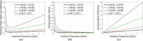
Structural damping of the bridge is modelled by Rayleigh Damping with the mass and stiffness proportional coefficients of μ = 0.02 and λ = 0.02. Then, the damping ratio is accordingly ξ = 0.5(μ/ω+λω). To address the effect and importance of the damping coefficients, the effect of different damping ratios are presented in Figure 3. For small angular frequencies, the mass proportional term is important, while with increasing angular frequencies, the effect of the stiffness term is becoming significant. The coefficients plotted are ranged from 0.01 to 0.1. It is obvious that the mass proportional term decreases while the stiffness proportional term increases with the increase in the angular frequency. With the above-mentioned Rayleigh damping coefficients, the structural damping is generally below 3% in the wave frequency range, which may be regarded as a reasonable assumption in view of the fact that other viscous effects, for example from the wind, are not considered in the numerical model.

Figure 3. Damping ratios for various angular frequencies under different mass proportional coefficients µ and stiffness proportional coefficients λ: (a) considering both µ and λ; (b) considering only µ; and (c) considering only λ.

The bridge girder is designed to be a truss structure. The steel truss work forms the key structural component of the floating bridge. In the numerical model, beam elements of equivalent flexural and torsional rigidity representing the truss configuration are employed. To evaluate the practical range of the flexural rigidity EIy and EIz, as well as the torsional rigidity GJ corresponding to a floating bridge, finite element models of truss work segments with various configurations and structural member sizes were constructed using the commercial software SAP2000 (Structures 2016), as shown in Figure 4. Note that in the truss structures, steel circular hollow sections with a diameter ranging from 600 to 1200 mm for the main chord members and 450 mm to 800 mm for the diagonal members are considered. These section sizes bear a close resemblance to the Bergsøysund Bridge in Norway (Kvåle et al. 2016). A variation in the size of the section and truss work configuration is also accounted for to cover a practical range of the bridge sectional properties. Analysis results show that the practical ranges of EIy, EIz and GJ are from 2×10⁶ MNm² to 10×10⁶ MNm², 2×10⁶ MNm² to 20×10⁶ MNm², and 1.23×10⁶ MNm²/rad to 10×10⁶ MNm²/rad, respectively. Based on the variations of the bridge girder's cross-sectional rigidity, different cases with three rigidity levels are selected for the analysis, represented by the number ‘I’, ‘II’ and ‘III’ shown in Table 2. Note that the degree of rigidity increases with the increase in the case number. Also note that in all cases, EA = 1×10⁶ MN remains constant.

Figure 4. Numerical model of various bridge girder cross-sections.

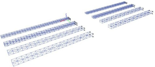
Table 2. Cases with different bridge girder cross-sectional rigidity and boundary conditions.

	EIy [×10^6 MNm^2]	EIz [×10^6 MNm^2]	EA [×10^6 MN]	GJ [×10^6 MNm^2/rad]	X	Y	Z	RX	RY	RZ
CASE IA	2	2	1	1.23	FIX	FIX	FIX	FIX	FIX	FIX
CASE IIA	6	10	1	5.23	FIX	FIX	FIX	FIX	FIX	FIX
CASE IIIA	10	20	1	10	FIX	FIX	FIX	FIX	FIX	FIX
CASE IB	2	2	1	1.23	FIX	FIX	FIX	FREE	FIX	FREE
CASE IIB	6	10	1	5.23	FIX	FIX	FIX	FREE	FIX	FREE
CASE IIIB	10	20	1	10	FIX	FIX	FIX	FREE	FIX	FREE

The boundary conditions or end connections will affect global stiffness properties. Two types of boundary conditions, i.e. rigid connection and flexible connection are considered to investigate the effect of the end connections. The rigid connection has fixed constraints on the 6 D.O.Fs at the two ends. The flexible connection allows rotation about the x and z axes (RX and RZ) in the global coordinate system. The end connection conditions are listed in Table 2, where cases with ‘A’ employ rigid end connections, while cases with ‘B’ adopt flexible end connections.

Time domain calculation is carried out by using the coupled SIMO-RIFLEX code, which was developed by Sintef Ocean (Previously MARINTEK). SIMO (MARINTEK 2009) is a code to simulate marine operations involving various bodies in the time domain. RIFLEX (MARINTEK 2013) is a code for analysis of slender marine structures. It is a nonlinear time domain programme with a finite element formulation that can handle large displacement and rotations. The pontoon motions are calculated in SIMO, while the slender bridge structural components are modelled by beam elements in RIFLEX. The model is a coupled hydro-structural dynamic model, where the pontoon motions and bridge girder responses are calculated and updated at a constant time step of 0.1 s.

2.2. Numerical verification

Under the bridge's self-weight and tide-induced water surface elevation, static deformation of the bridge girder occurs. A tidal variation of ±2 m is accounted for in the analysis. Since the tide-induced water surface variation is usually very slow, such effects can be reasonably taken as a static process. In addition, tidal effects are considered in a simplified way by applying a stiffness force due to the tide-induced water surface elevation to the pontoons. However, it should be clarified that the force is not a pre-defined constant as it also depends on the pontoon draft changes due to the stiffness of the bridge structure. This draft change is different for various cases. This may introduce limited uncertainties. In the floating bridge engineering design, there are some special considerations catered for the tidal variation effects, e.g. a transition piece at the end of the bridge can be installed to allow the bridge girder to deform due to the tidal variations. Nevertheless, no transition piece is considered in the current stage of the study.

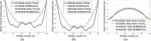
The numerical results are attempted to be verified through comparison with an analytical solution based on a uniform Euler beam model. The analytical solution is presented in the Appendix. Results for verification results regarding the static vertical bending moment and deformation of straight bridges are shown in Figure 5. For curved bridges, the results are presented in Figure 6. It is seen that a perfect match is achieved for straight bridges, and excellent agreement is also observed for curved bridges. These validate the accuracy of the numerical model.

Figure 5. Analytical and numerical results of static vertical bending moment for case RINFIB (a), of static vertical deformation for case RINFIB under self-weight (b); and of static vertical deformation for cases RINFIB and RINFIIIB under tidal position of +2 m (c).

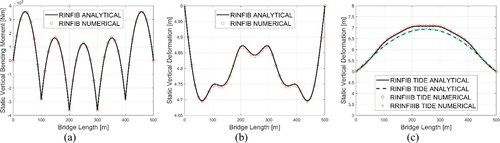
Figure 6. Analytical and numerical results of static vertical deformation for cases R1000IB and R1000IIIB (a), and cases R500IB and R500IIIB (b) under self-weight; and of static vertical deformation for cases R1000IB and R1000IIIB under tidal position of +2 m (c).

3. Results and analysis

3.1. Responses induced by self-weight, current and tidal variation

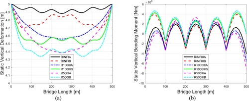
Static vertical deformation and vertical bending moment along the bridge length under the bridge self-weight are shown in Figure 7. Only the cross-section for case I is investigated. Since it represents the lowest cross-sectional properties, the largest deformations among all the cases considered are expected. All the three bridge curvatures with the two different end connections are considered. It is found that the straight bridges (RINF) tend to have the smallest static deformation, followed by curved bridges R1000 and R500. Fixed boundary condition results in much smaller static deformations when compared with flexible boundary condition. The maximum static deformation is less than 0.7 m for Case I and is expected to be smaller for Cases II and III. Note that this maximum deformation of 0.7 m only corresponds to 0.14% of the total bridge length, thus it may be regarded as negligible. The static vertical bending moment shows that the fixed boundary condition (Cases A) induces large bending moments especially in the end spans between the shoreline and the end pontoons (PT1 and PT4). The bridge curvature is found to have limited effects on the static bending moment along the bridge girder.

Figure 7. Static vertical deformation for cases with cross-section I (a), and static vertical bending moment for cases with cross-section III (b) along the bridge length under self-weight.

Current forces are treated as static forces and are applied to the pontoons to study the induced responses. A current quadratic coefficient of 0.9 is used. The horizontal displacements of PT1 and PT2 in the global X direction (pontoon surge D.O.F) caused by the current in Case IB are found to be 0.10 and 0.17 m, respectively, which are deemed small and negligible. For other cases where the bridge girder is much stiffer, the current induced deflection is even smaller. Thus, it may be concluded that the current only has a marginally effect on the bridge response.

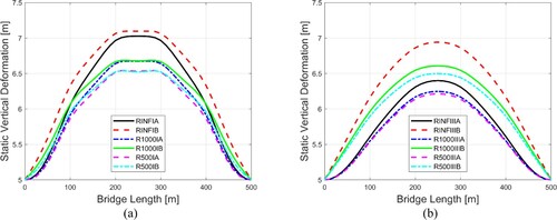
At a +2 m tidal condition, the static vertical deformations of the bridge with cross-sections considered in cases I and III are plotted in Figure 8. It is observed that the largest vertical deformation is about 2 m for case I, while for case III, the deformation is significantly reduced. The deformed shape along bridge length appears to be smoother for cases III due to the stiffer cross-sectional properties. It can also be seen that the straight bridge has the largest deformation, followed by curved bridges of a radius of 1000 m and subsequently 500 m. This clearly shows that large curvature can reduce the tide-induced bridge deformations. In addition, the fixed boundary condition can also help reduce the deformation, but the reduction effect is more profound for cases III than cases I. It is noted that the tide-induced static deformation may introduce geometrical nonlinearities in the bridge girder and thus affects the dynamic responses.

Figure 8. Static vertical deformation of the floating bridges for cases with cross-section I (a), and cases with cross-section III (b) under tidal position of +2 m.

3.2. Modal parameter identification

The modal properties of the bridges are affected by the cross-sectional properties, boundary conditions as well as the radius of curvature. Eigen value analysis is carried out for different cases listed in Table 2. The first ten eigen periods identified are listed in Table 3 which cover the resonant periods as low as 1 s. It is obvious that by increasing the bridge cross-sectional rigidity, i.e. from case I to case III, the eigen periods decrease. In the meanwhile, it is important to notice that with the increase in the curvature of the bridge, the variation of the eigen periods due to the change in the cross-sectional rigidity is not significant. This implies the importance of the curvature of the bridge. By comparing Case B with Case A, it is noted that the flexible boundary condition would also increase the eigen periods of the bridge. This is expected in view that the imposed boundary condition softens the overall stiffness of the bridge structure.

Table 3. Identified eigen periods for the cases listed in Table 2.

	CASE IA			CASE IIA			CASE IIIA
	R ∞ [s]	R1000 [s]	R500 [s]	R ∞ [s]	R1000 [s]	R500 [s]	R ∞ [s]	R1000 [s]	R500 [s]
1	12.89	7.42	7.53	6.56	6.62	6.81	5.96	6.03	6.26
2	7.39	5.47	5.70	5.78	3.82	4.04	4.09	3.10	3.30
3	5.40	4.90	5.46	3.75	2.21	2.44	3.04	1.82	1.85
4	4.74	3.55	3.76	2.17	2.19	2.35	1.71	1.74	1.73
5	3.50	3.54	3.40	2.12	2.03	1.89	1.50	1.55	1.41
6	3.50	2.91	3.01	1.95	1.86	1.66	1.44	1.43	1.30
7	2.55	2.59	2.75	1.53	1.56	1.42	1.20	1.22	1.11
8	2.48	2.11	2.08	1.11	1.09	1.05	0.79	0.79	0.77
9	2.09	1.72	1.79	1.06	1.07	0.85	0.77	0.78	0.75
10	1.62	1.66	1.58	0.77	0.79	0.81	0.56	0.57	0.57
	CASE IB			CASE IIB			CASE IIIB
	R ∞ [s]	R1000 [s]	R500 [s]	R ∞ [s]	R1000 [s]	R500 [s]	R ∞ [s]	R1000 [s]	R500 [s]
1	28.09	7.85	8.68	13.02	7.65	7.77	9.23	7.46	7.63
2	7.81	7.62	7.91	7.60	5.16	5.44	7.40	4.38	4.67
3	7.30	6.58	6.80	5.07	3.42	3.88	4.30	2.42	2.75
4	6.51	4.38	4.62	3.29	2.83	3.02	2.33	2.25	2.41
5	4.29	3.65	3.89	2.78	2.04	1.89	2.21	1.85	1.45
6	3.50	3.50	3.40	1.95	1.87	1.86	1.44	1.43	1.41
7	3.30	2.88	3.05	1.71	1.74	1.76	1.34	1.36	1.28
8	2.82	2.11	2.11	1.48	1.39	1.05	1.05	1.04	0.82
9	2.09	1.95	2.08	1.06	1.07	0.95	0.77	0.78	0.77
10	1.90	1.74	1.59	0.86	0.88	0.86	0.61	0.62	0.67

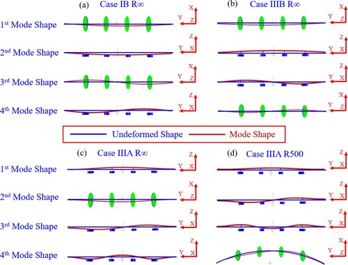
The first four eigen mode shapes for some selected cases are shown in Figure 9. The top subplots in Figure 9 show the Case IB and Case IIIB corresponding to a straight bridge (R = ∞). The first four modes include two horizontal modes (in the X-Y plane) and two vertical modes (in the Y-Z plane). Note that some mode shapes are similar to each other, but the order of the mode shapes may be different. On the bottom subplots in Figure 9, eigen mode shapes for Case IIIA are shown with different bridge curvatures, i.e. R = ∞ and R = 500 m. It is found that the order of the mode shapes is varied, but the mode shapes are quite similar. Important eigen periods of the bridge in this study cover a range from 30 s (0.2 rad/s) to 1 s (6.28 rad/s). When this is read in conjunction with Figure 3, the structural damping ratios are mostly below 0.1. Moreover, m the fundamental eigen periods are between 2 and 10 s, where the structural damping ratios are below 0.05.

Figure 9. The first four eigen mode shapes of the floating bridge: (a) Case RINFIB; (b) Case RINFIIIB; (c) Case RINFIIIA; (d) Case R500IIIA.

It should be highlighted that the above-mentioned eigen properties do not consider the frequency-dependent added mass, which may impose some uncertainties in the estimation of the ‘wet’ mode periods. When a reference is made to a 4600 m long floating bridge with discrete pontoons (Cheng et al. 2018a), the largest error due to the neglection of the frequency-dependent added mass is 10% and is for its first eigen period which is about 57 s. For the subsequent eigen periods, the error varies between 0.1 and 7%. For the floating bridges considered in the current study, the longest eigen period is 28 s only. For this reason, the effect of added mass on the eigen periods is expected to be much smaller, which implies that the uncertainties due to the neglection of the frequency-dependent added mass are limited.

3.3. Regular wave analysis

Regular wave analysis is performed to investigate the dynamic responses of the bridges at different excitation frequencies. In this study, the spectral approach is applied, i.e. a white noise spectrum with frequency ranging from 0.2 to 3.14 rad/s (period range of 2–31.4 s) and with a uniform spectral amplitude of 1 m²s/rad is used to excite the bridges. The Response Amplitude Operators (RAOs) are then calculated by the square root of the ratio between the output response spectra and the input wave spectrum. Zero-degree incoming wave direction as indicated in Figure 2 is used for the regular wave analysis. In this session, the surge, heave and pitch motions of the pontoons as well as the axial forces, vertical bending moments and vertical shear forces of the bridge girder at the pontoon positions and at the two bridge ends are investigated. The response RAOs are presented and discussed below.

Firstly, the curvature effects are studied for Case IB with a change in the bridge curvature from R = ∞ to R = 500 m. The pontoon motion response RAOs are plotted in Figure 10, while the structural responses of the bridge girder are shown in Figure 11. It is seen from Figure 10 that the surge motion of the two pontoons, i.e. PT1 and PT2, are significantly reduced due to the increase in the bridge curvature. However, the heave and pitch motions are not strongly affected. PT1 generally has smaller motions than PT2 due to its proximity to the bridge end. Under the action of long waves where the wave frequency is close to zero, the heave motion of PT2 would follow the wave motion, and thus the RAO is close to 1. From Figure 11, the axial forces for straight bridges are much larger than the curved bridges, and the axial forces at End1 and PT1 positions are identical for the same case. The vertical bending moment at End1 is zero due to the pre-defined pinned condition.

Figure 10. RAOs of surge (a), heave (b), and pitch (c) motions of PT1 and PT2, for Cases RINFIB and R500 IB.

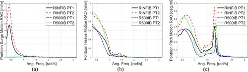
Figure 11. RAOs of axial force (a), vertical bending moment (b), and vertical shear force (c) of bridge girder at End 1 and PT1 position, for Cases RINF IB and R500IB.

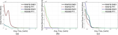
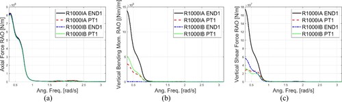
Secondly, the boundary condition effects are investigated for bridges with a radius of 1000 m (R1000IA and R1000IB). Motion and structural response RAOs are plotted in Figures 12 and 13. From Figure 12, the surge RAOs are below unity and have different peaks that correspond to the various structural eigen modes. Also, surge motions are generally larger for bridges with flexible end connection (Cases B) except for specific modes that are found to be excited only for Cases A; Heave motions for PT1 and PT2 are slightly higher when the end connections are flexible. Pitch motions have similar peak frequencies and the responses are higher for bridges with flexible end connections. As can be seen in Figure 13, the axial forces are virtually unaffected by the end connections. The vertical bending moment at the bridge ends is larger than that at the PT1 position for bridges with fixed end connections. Similarly, vertical shear forces at the end are significantly larger than for bridges with fixed end connections.

Figure 12. RAOs of surge (a), heave (b) and pitch (c) motions of PT1 and PT2, for Cases R1000IA and Case R1000IB.

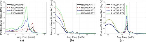
Figure 13. RAOs of axial force (a), vertical bending moment (b), and vertical shear force (c) of bridge girder at End 1 and PT1 position, for Cases R1000IA and R1000IB.

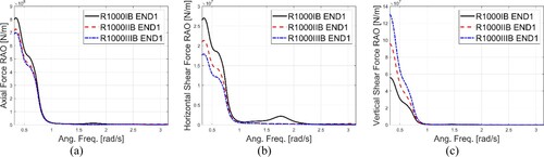
The effect of bridge cross-sectional rigidity is next studied for Cases R1000I, R1000II and R1000III considering flexible end connections. The results are shown in Figures 14 and 15. As shown in Figure 14, only motions corresponding to PT2 are presented, and clearly that the increase in the cross-sectional rigidity decreases the motion responses. Also, it is obvious that if small pontoon motions should be achieved, sectional properties presented in Cases II and III should be considered in the design. Figure 15 shows the structural responses including the axial force, horizontal and vertical shear forces at End1 position. Results reveal that with the increase in the cross-sectional rigidity, the axial forces and horizontal shear forces decrease while the vertical shear forces increase.

Figure 14. RAOs of surge (a), heave (b), and pitch (c) motions of PT 2, for Cases R1000IB, R1000IIB and R1000IIIB.

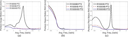
Figure 15. RAOs of axial force (a), horizontal (b) and vertical shear force (c) of bridge girder at End 1 position, for Cases R1000IB, R1000IIB and R1000IIIB.

From the regular wave analysis, the curved bridge is shown to be able to significantly reduce the pontoon surge motions as well as the axial force in the bridge girder. But the curvature in the bridge girder also leads to an increase in the vertical bending moment and shear force. The end connections also affect the pontoon motions. When an increase in the bridge cross-sectional rigidity, the pontoon surge and pitch motions can be significantly reduced.

3.4. Irregular wave analysis

Floating bridges should be carefully designed such that they are comfortable to ride on during operational (1-year storm) conditions and they should avoid undesirable structural damages during extreme storm (100-year storm) conditions (Lwin 2000). Motion responses of floating bridges affect their functionality and thus are important driving parameters in the design. Under operational conditions, the wave-induced deflection should not exceed ±0.3 m in both surge and heave directions, and ±0.5 degrees in pitch. Meanwhile, the acceleration due to wave loads should not exceed ±0.5 m/s², ±0.5 m/s² and ±0.05 rad/s² (±2.87 degree/s²) in the surge, heave and pitch D.O.Fs, respectively (Lwin 2000). Under extreme storm conditions, the bridge should be designed to survive with the road closure.

The two curved bridges with R = 1000 m and R = 500 m are selected for detailed study in this section. In addition, pinned boundary conditions are more feasible when compared with fully fixed end conditions due to lower reaction forces, and thus they are adopted for the parametric studies. In terms of the cross-sectional properties, Case I (‘soft’ cross-section) is expected to sustain larger motions and therefore not considered here. Hence, Cases B with the cross-section types ‘II’ and ‘III’, together with the above-mentioned two bridge radii are the central focus in the irregular wave analysis. Time domain simulations with a length of 4000 s are carried out, in which 1-hour steady-state results will be used for detailed examination. Motion statistics like the mean (MEAN), maximum (MAX), standard deviation (STD) and minimum (MIN) values are presented and discussed. Spectral analysis is also performed.

Two water surface elevations are considered. The neutral position of 0 m represents the condition without tidal effect, while +2 m refers to the high tide condition where the water surface is elevated by 2 m. The latter is denoted as ‘TD’ in the study. When the tidal effect is present, the induced static deformation may alter the global stiffness of the floating bridges, and consequently, the dynamic responses under irregular wave conditions could be different.

Motion responses of PT2 for R500IIB and R500IIIB under operational wave conditions with and without tidal variations are shown in Figure 16. It can be seen that the tidal variations lead to significant changes in the MEAN, MAX. and MIN. values of the surge, heave and pitch motions. But the STD values are only slightly affected. This indicates that the static response due to the bridge's self-weight and tidal effects governs. In general, the motion magnitudes are quite small, especially of surge and pitch, which are less than 0.02 m and 0.5 degrees, respectively. Heave motion is also small when referred to the differences between the MAX or MIN and MEAN values. Clearly, the motions of the bridge girders satisfy the functionality requirements under operational conditions.

Figure 16. Statistical values (MEAN, STD, MAX and MIN) of surge (a), heave (b), and pitch (c) motions of PT2 for Cases R500IIB and R500IIIB under operational (OPR) conditions with and without tidal (TD) variation effect.

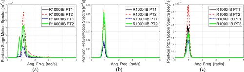
Motion spectra of PT1 and PT2 for R1000IIB and R1000IIIB under extreme wave conditions are plotted in Figure 17. It can be seen that the motions of PT2 are larger than that of PT1. Also, the pontoon motions are generally smaller with cross-section III instead of cross-section II. The power of responses is mostly concentrated near the wave excitation frequency (1.08 rad/s). In the surge responses, there is a prominent peak at around 0.8 rad/s, which corresponds to the first eigen period of bridges R1000B.

Figure 17. Spectra of surge (a), heave (b) and pitch (c) motions of PT1 and PT2, for Cases R1000IIB and R1000IIIB under extreme conditions.

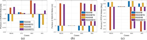
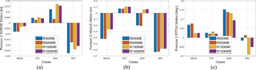
The motion statistics of PT2 under extreme wave conditions are shown in Figure 18. It can be seen that the absolute mean values are larger for R500 bridges, which may be explained as due to the larger overall length of the bridges with a smaller radius and thus higher self-weight. The STD for Cases III bridges is clearly smaller than Cases II bridges. Similarly, the STD for R500 bridges is also smaller than R1000 bridges.

Figure 18. Statistical values (MEAN, STD, MAX and MIN) of surge (a), heave (b), and pitch (c) motions of PT2 for cases R500IIB, R500IIIB, R1000IIB and R1000IIIB under extreme wave conditions.

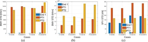
To study the tidal effects on the bridge responses under extreme conditions, cases R1000IIB and R1000IIIB are investigated with and without the 2 m tide. The statistics of the surge, heave and pitch motions for PT2 are shown in Figure 19. Due to tidal variations, the mean motions of PT2 are strongly affected; the STDs of surge and pitch motions are amplified and reduced, respectively. However, heave STDs are not significantly influenced. Similar results are observed for R500 bridges as presented in Figure 16. The tidal effects on structural reaction forces are shown in Figure 20, where STDs of the vertical and horizontal bending moments as well as the vertical shear force at End1, PT1 and PT2 positions are presented. It can be seen that due to the 2 m tide, the vertical bending moment is slightly reduced, while the horizontal bending moment is amplified. The change in the vertical shear force, however, is negligible.

Figure 19. Statistical values (MEAN, STD, MAX and MIN) of surge (a), heave (b), and pitch (c) motions of PT2 for cases R1000IIB and R1000IIIB under extreme conditions with and without tidal variation effect.

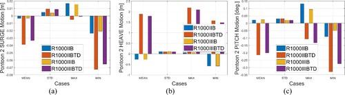
Figure 20. Statistical values (MEAN, STD, MAX and MIN) of horizontal bending moment (a), vertical bending moment (b), and vertical shear force (c) of bridge girder at End1, PT1 and PT2 positions, for cases R1000IIB and R1000IIIB under extreme conditions with and without tidal variation effect.

4. Conclusions and discussion

Three short-span curved floating bridges for the crossing the shallow coastal waters in Singapore are proposed and studied. These bridges have a total span of 500 m, and they are vertically supported by 4 discrete pontoons. To cater to the local high traffic demand, the bridge girder is designed to carry dual-way three-lane carriageways, leading to a relatively high stiffness in the horizontal plane. These features make the bridge designs presented in this paper quite different from the existing floating bridges around the world. Three bridges with different radii of curvature are studied, i.e. a straight bridge, a bridge with a radius of 1000 m and a bridge with a radius of 500 m. Coupled hydro-structural dynamic models are established. The accuracy of the numerical models is verified by comparison with an analytical solution. Various critical parameters are studied, including the bridge cross-sectional properties, end connection conditions, as well as the radii of curvature. The results and findings from the current study could provide useful insights into the design parameters in the initial design phase.

Static deformations due to the bridge's self-weight, current and tidal effects are firstly investigated. An analytical model is presented and used to verify the numerical results. Very good agreements between the analytical and numerical results are found, thereby validating the accuracy of the proposed numerical models. In the examination of various static load effects, the current is found to be marginally important. The straight bridge has the smallest vertical static deformation, followed by R1000 and then R500, and bridges with flexible boundary conditions have larger deformations. The maximum static vertical deformation is less than 0.7 m for all the bridge configurations considered. When tidal variations are present, large curvature and fixed end connections can effectively reduce the tide-induced deformations. Such a reduction effect is more significant for bridges with stiffer cross-sections.

The eigen value analysis shows that the eigen periods of the bridges can be reduced by employing rigid end connections and increasing the girder's cross-sectional rigidity. With an increase in the bridge curvature, the change in the eigen periods due to the cross-sectional rigidity is not so significant. This indicates that the presence of curvature in the bridge effectively increases the stiffness in the curvature plane. However, the fundamental mode shapes are not strongly influenced by these design parameters in the current study.

Regular wave analysis is carried out to investigate the response amplitude operators (RAOs) of the response parameters. The study on the curvature effects shows that the pontoon surge motion is significantly reduced due to the bridge curvature, while the influence on the heave and pitch motions are limited. The axial force responses are larger for the straight bridge than curved bridges. By studying the end connection effects, it is found that the pontoon surge, heave and pitch motions are generally larger when flexible end connections are employed, while the axial forces are virtually unaffected. From the investigation of three cross-sections of the bridge girder, it is found that with the increase in the sectional rigidity, the pontoon motion responses and axial forces as well as the horizontal shear forces at the end position, are reduced, while the vertical shear forces are increased.

Irregular wave analysis reflects the performance of the floating bridges under realistic environmental conditions. Two curved bridge configurations with R = 1000 m and R = 500 m together with two relatively stiff girder cross-sections (Cases II and III) are selected for detailed study. Under operational conditions, all pontoon motions are pretty small. Under extreme conditions, the dynamic pontoon motions for case III bridges are smaller than case II bridges. The spectral analysis of R1000IIB and R1000IIIB bridges shows that the power of the pontoon motions is mainly concentrated in the vicinity of the wave frequencies.

The work reported in this paper focuses on short-span floating curved bridges, with a variety of different design parameters in the practical range. These parameters have an impact on the dynamic properties of the bridges. Through this study, the importance of these design parameters is addressed. However, it should be mentioned that the motion responses under operational conditions and the structural integrity under survival conditions need further assessment according to various design criteria. For larger and longer floating bridges that are not the focus of this study, their dynamic properties can be quite different, and thus further studies are needed to draw more general conclusions and recommendations on the design.

Acknowledgement

This research is supported partly by the Singapore Ministry of National Development and the National Research Foundation, Prime Minister's Office under the Land and Liveability National Innovation Challenge (L2 NIC) Research Programme (L2 NIC Award No L2 NICTDF1-2015-2). Any opinions, findings, and conclusions or recommendations expressed in this material are those of the author(s) and do not reflect the views of the Singapore Ministry of National Development and National Research Foundation, Prime Minister's Office, Singapore. The authors also gratefully acknowledge the research funding supports from Newcastle University through Newcastle Research & Innovation Institute Pte Ltd (NewRIIS), Singapore, as well as funding supports from Natural Science Foundation of Jiangsu Province under grant number BK20180487 and National Natural Science Foundation of China (NSFC) under grant number 51808292.

Disclosure statement

No potential conflict of interest was reported by the author(s).

Additional information

Funding

This work was supported by Natural Science Foundation of Jiangsu Province: [Grant Number BK20180487]; Land and Liveability National Innovation Challenge (L2 NIC): [Grant Number L2 NICTDF1-2015-2]; National Natural Science Foundation of China (NSFC): [Grant Number 51808292].

Appendix

A.1.#Analytical model

The floating bridge presented in this paper is a complex system subject to static loads and dynamic excitations arising from imposed and environmental loads. In a calm sea condition, the bridge girder mainly undergoes static deformation in the vertical direction due to its self-weight and tide-induced water surface change. Attempting to verify the static response of the floating bridge predicted by the numerical model, a curved uniform Euler beam model shown in Figure 21 is considered where an analytical solution can be developed. The beam has a length L, radius R, cross-sectional area A, density ρ and flexural rigidity EI_y, and is discretely supported by springs of hydrostatic stiffness at pontoon positions. The governing equations of the bridge displacements out of its curvature plane under self-weight and tide-induced water surface change are given by (A1) $E{I}_y{\displaystyle \frac{{\mathrm{\partial }}^{4}w}{\mathrm{\partial }{x}^4}-{\displaystyle \frac{1}{R}{\displaystyle \frac{{\mathrm{\partial }}^2\beta }{\mathrm{\partial }{x}^2}-{\displaystyle \frac{GJ}{R}\left({\displaystyle \frac{1}{R}{\displaystyle \frac{{\mathrm{\partial }}^{2}w}{\mathrm{\partial }{x}^2}+{\displaystyle \frac{{\mathrm{\partial }}^2\beta }{\mathrm{\partial }{x}^2}}}}\right)+\sum _{k=1}^{N_p}{k}_h(w-H_T-d)\delta (x-x_k)=-\rho Ag}}}}$(A1) (A2) ${\displaystyle \frac{E{I}_x}{R}\left({\displaystyle \frac{\beta }{R}-{\displaystyle \frac{{\mathrm{\partial }}^{2}w}{\mathrm{\partial }{x}^2}}}\right)-GJ\left({\displaystyle \frac{{\mathrm{\partial }}^2\beta }{\mathrm{\partial }{x}^2}+{\displaystyle \frac{1}{R}{\displaystyle \frac{{\mathrm{\partial }}^{2}w}{\mathrm{\partial }{x}^2}}}}\right)+\sum _{k=1}^{N_p}{k}_t\beta \delta (x-x_k)=0}$(A2) where w is the vertical displacement and torsional deformation, β is the torsional rotation, k_h is the vertical hydrostatic stiffness, k_t is the torsional hydrostatic stiffness, N_p refers to the number of pontoons, x_k is the location of pontoon k along x-axis, H_T is the tide induced water surface elevation, and d is the initial draft of pontoons. In view of the boundary conditions and the coupled relationship between w and β, the vertical and torsional deformation of the beam can be expressed as the summation of a series of sinusoidal functions as (A3) $w=\sum _{i=1}^n{q}_{wi}\sin {\displaystyle \frac{i\pi x}{L}}$(A3) (A4) $\beta =\sum _{i=1}^n{q}_{\beta i}\sin {\displaystyle \frac{i\pi x}{L}}$(A4) where q_wi and q_βi denote the generalised coordinates of ith mode, and n is the number of modes included in the computation. By employing Galerkin's approach to formulate the weighted residual form of Equation A1 (Dai and Ang 2015), the generalised coordinates can be obtained by solving the following modal governing equations corresponding to the ith mode: (A5) $\sum _{j=1}^n{a}_{ij}{q}_{wj}+b_{ii}{q}_{\beta j}=\sum _{k=1}^{N_p}{\displaystyle \frac{2k_h}{L}(H_T+d)\sin {\displaystyle \frac{i\pi x_k}{L}}}-{\displaystyle \frac{2\rho gA}{i\pi }(1-\cos i\pi )}$(A5) (A6) $\sum _{j=1}^n{c}_{ij}{q}_{\beta j}+d_{ii}{q}_{wj}=0$(A6) where the modal coefficient a_ij is given by (A7) $a_{ij}=\{\begin{array}{c}E{I}_y{\left({\displaystyle \frac{i\pi }{L}}\right)}^4+\sum _{k=1}^{N_p}{\displaystyle \frac{2k_h}{L}\sin \left({\displaystyle \frac{i\pi x_k}{L}}\right)\sin \left({\displaystyle \frac{j\pi x_k}{L}}\right),\mathrm{if}i=j}\\ \sum _{k=1}^{N_p}{\displaystyle \frac{2k_h}{L}\sin \left({\displaystyle \frac{i\pi x_k}{L}}\right)\sin \left({\displaystyle \frac{j\pi x_k}{L}}\right)},\mathrm{if}i\ne j\end{array}$(A7) (A8) $b_{ii}={\displaystyle \frac{1}{R}(E{I}_y+GJ){\left({\displaystyle \frac{i\pi }{L}}\right)}^2}$(A8) (A9) $c_{ij}=\{\begin{array}{c}{\displaystyle \frac{E{I}_y}{R}+GJ{\left({\displaystyle \frac{i\pi }{L}}\right)}^2+\sum _{k=1}^{N_p}{\displaystyle \frac{2k_t}{L}\sin \left({\displaystyle \frac{i\pi x_k}{L}}\right)\sin \left({\displaystyle \frac{j\pi x_k}{L}}\right),\mathrm{if}i=j}}\\ \sum _{k=1}^{N_p}{\displaystyle \frac{2k_t}{L}\sin \left({\displaystyle \frac{i\pi x_k}{L}}\right)\sin \left({\displaystyle \frac{j\pi x_k}{L}}\right)},\mathrm{if}i\ne j\end{array}$(A9) (A10) $d_{ii}={\displaystyle \frac{1}{R}(E{I}_y+GJ){\left({\displaystyle \frac{i\pi }{L}}\right)}^2}$(A10)

Figure 21. Simplified curved bridge model.

Subsequently, the bending moment about the weak axis of the bridge girder can be evaluated using Equation A11: (A11) $M_y=-E{I}_y\sum _{i=1}^n{\left({\displaystyle \frac{i\pi }{L}}\right)}^2{q}_{wi}\sin {\displaystyle \frac{i\pi x}{L}}$(A11) Note that when the radius R is set to zero, the coupling between the vertical and torsional deformations of the bridge girder vanishes and the abovementioned analytical solution reduces to the conventional solution to a straight floating bridge.

References

- 16th ISSC COMMITTEE VI.2. 2006. Very large floating structures.
- Cheng Z, Gao Z, Moan T. 2018a. Hydrodynamic load modeling and analysis of a floating bridge in homogeneous wave conditions. Mar Struct. 59:122–141.
- Cheng Z, Gao Z, Moan T. 2018b. Wave load effect analysis of a floating bridge in a fjord considering inhomogeneous wave conditions. Eng Struct. 163:197–214.
- Cheng Z, Svangstu E, Gao Z, Moan T. 2018c. Field measurements of inhomogeneous wave conditions in Bjørnafjorden. J Waterway Port Coast Ocean Eng. 145(1):05018008.
- Cummins W. 1962. The impulse response function and ship motions. SchiffStechnik. 47(9):101–109.
- Dai J, Ang KK. 2015. Steady-state response of a curved beam on a viscously damped foundation subjected to a sequence of moving loads. Proc Inst Mech Eng F J Rail Rapid Transit. 229(4):375–394.
- Dai J, Ang KK, Jin J, Wang CM, Hellan Ø, Watn A. 2019. Large floating structure with free-floating, self-stabilizing tanks for hydrocarbon storage. Energies. 12:3487.
- Dai J, Leira BJ, Moan T, Alsos HS. 2021a. Effect of wave inhomogeneity on fatigue damage of mooring lines of a side-anchored floating bridge. Ocean Engineering. 219:108304. https://doi.org/10.1016/j.oceaneng.2020.108304.
- Dai J, Leira BJ, Moan T, Kvittem MI. 2020a. Inhomogeneous wave load effects on a long, straight and side-anchored floating pontoon bridge. Mar Struct. 72:102763.
- Dai J, Stefanakos C, Leira BJ, Alsos HS. 2021b. Effect of Modelling Inhomogeneous Wave Conditions on Structural Responses of a Very Long Floating Bridge. Journal of Marine Science and Engineering. 9(5):548. https://doi.org/10.3390/jmse9050548.
- Dai J, Wang CM, Utsunomiya T, Duan W. 2018. Review of recent research and developments on floating breakwaters. Ocean Engineering. 158:132–151. https://doi.org/10.1016/j.oceaneng.2018.03.083.
- Dai J, Zhang C, Lim HV, Ang KK, Qian X, Wong JLH, Tan ST, Wang CL. 2020b. Design and construction of floating modular photovoltaic system for water reservoirs. Energy. 191:116549.
- DNV. 2010. Recommended practice dnv-rp-c205, environmental conditions and environmental loads.
- Faltinsen OM. 1993. Sea loads on ships and offshore structures. Cambridge, UK: Cambridge University Press.
- Fu S, Cui W-C, Chen X, Wang C. 2005. Hydroelastic analysis of a nonlinearly connected floating bridge subjected to moving loads. Mar Struct. 18(1):85–107.
- Gao Z, Moan T, Wan L, Michailides C. 2016. Comparative numerical and experimental study of two combined wind and wave energy concepts. J Ocean Eng Sci. 1:36–51.
- Jiang D, Tan KH, Dai J, Ang KK, Nguyen HP. 2021a. Behavior of concrete modular multi-purpose floating structures. Ocean Engineering. 229:108971. https://doi.org/10.1016/j.oceaneng.2021.108971.
- Jiang D, Tan KH, Dai J, Ong KCG, Heng S. 2019. Structural performance evaluation of innovative prestressed concrete floating fuel storage tanks. Structural Concrete. 20(1):15–31. https://doi.org/10.1002/suco.2019.20.issue-1.
- Jiang D, Tan KH, Wang CM, Dai J. 2021b. Research and development in connector systems for very large floating structures. Ocean Engineering. 232:109150. https://doi.org/10.1016/j.oceaneng.2021.109150.
- Jiang D, Tan KH, Wang CM, Ong KCG, Bra H, Jin J, Kim M. 2018. Analysis and design of floating prestressed concrete structures in shallow waters. Mar Struct. 59:301–320.
- Karimirad M, Moan T. 2012. A simplified method for coupled analysis of floating offshore wind turbines. Mar Struct. 27(1):45–63.
- Kashiwagi M. 2000. Research on hydroelastic responses of VLFS: recent progress and future work. Int J Offshore Polar Eng. 10(2):81–90.
- Kashiwagi M. 2004. Transient responses of a VLFS during landing and take-off of an airplane. J Mar Sci Technol. 9(1):14–23.
- Kvåle KA, Sigbjörnsson R, Øiseth O. 2016. Modelling the stochastic dynamic behaviour of a pontoon bridge: a case study. Comput Struct. 165:123–135.
- Løken A, Oftedal R, Aarsnes J. 1990. Aspects of hydrodynamic loading and responses in design of floating bridges. Presented at Second Symposium on Strait Crossings, Trondheim, Norway, June.
- Lwin M. 2000. Floating bridges. Bridge Eng Handb. 22:1–23.
- MARINTEK. 2009. SIMO – theory manual version 3.6, rev: 2.
- MARINTEK. 2013. Riflex theory manual v4.0 rev3.
- Michailides C, Gao Z, Moan T. 2016. Experimental and numerical study of the response of the offshore combined wind/wave energy concept SFC in extreme environmental conditions. Mar Struct. 50:35–54.
- Naess A, Moan T. 2013. Stochastic dynamics of marine structures. New York, USA: Cambridge University Press.
- Petersen ØW, Øiseth O. 2017. Sensitivity-based finite element model updating of a pontoon bridge. Eng Struct. 150:573–584.
- Seif MS, Inoue Y. 1998. Dynamic analysis of floating bridges. Mar Struct. 11(1):29–46.
- Sha Y, Amdahl J. 2019. Numerical investigations of a prestressed pontoon wall subjected to ship collision loads. Ocean Eng. 172:234–244.
- Sha Y, Amdahl J, Dørum C. 2019. Local and global responses of a floating bridge under ship–girder collisions. J Offshore Mech Arct Eng. 141(3):031601.
- Solland G, Haugland S, Gustavsen JH. 1993. The Bergsøysund Floating Bridge, Norway. Struct Eng Int. 3(3):142–144.
- Structures C. 2016. CSI analysis reference manual, rev. 15. Berkeley, California.
- Viuff T, Xiang X, Øiseth O, Leira BJ. 2020. Model uncertainty assessment for wave- and current-induced global response of a curved floating pontoon bridge. Appl Ocean Res. 105:102368.
- Wan L, Gao Z, Moan T. 2015. Experimental and numerical study of hydrodynamic responses of a combined wind and wave energy converter concept in survival modes. Coastal Eng. 104:151–169.
- Wan L, Gao Z, Moan T, Lugni C. 2016. Experimental and numerical comparisons of hydrodynamic responses for a combined wind and wave energy converter concept under operational conditions. Renew Energy. 93:87–100.
- Wan L, Greco M, Lugni C, Gao Z, Moan T. 2017a. A combined wind and wave energy-converter concept in survival mode: numerical and experimental study in regular waves with a focus on water entry and exit. Appl Ocean Res. 63:200–216.
- Wan L, Han M, Jin J, Zhang C, Magee AR, Hellan Ø, Wang CM. 2018. Global dynamic response analysis of oil storage tank in finite water depth: focusing on fender mooring system parameter design. Ocean Eng. 148:247–262.
- Wan L, Magee AR, Hellan Ø, Arnstein W, Ang KK, Wang CM. 2017b. Initial design of a double curved floating bridge and global hydrodynamic responses under environmental conditions. Presented at Proceedings of the ASME 2017 36th International Conference on Ocean, Offshore and Arctic Engineering, OMAE2017-61802, June 25–30, 2017, Trondheim, Norway.
- Watanabe E, Utsunomiya T. 2003. Analysis and design of floating bridges. Prog Struct Mat Eng. 5(3):127–144.
- Watanabe E, Utsunomiya T, Wang CM. 2004a. Hydroelastic analysis of pontoon-type VLFS: a literature survey. Eng Struct. 26(2):245–256.
- Watanabe E, Utsunomiya T, Wang CM, Xiang Y. 2003. Hydroelastic analysis of pontoon-type circular VLFS. Presented at The Thirteenth International Offshore and Polar Engineering Conference.
- Watanabe E, Wang C, Utsunomiya T, Moan T. 2004b. Very large floating structures: applications, analysis and design. CORE Report. 2:104–109.
- Wu M, Moan T. 1996. Linear and nonlinear hydroelastic analysis of high-speed vessels. J Ship Res. 40(2):149–163.
- Xu Y, Øiseth O, Moan T. 2017. Time domain modelling of frequency dependent wind and wave forces on a three-span suspension bridge with two floating pylons using state space models. Presented at ASME 2017 36th International Conference on Ocean, Offshore and Arctic Engineering.