A novel framework for imputing large gaps of missing values from time series sensor data of marine machinery systems

ABSTRACT

Condition-based maintenance is a maintenance strategy that implements Industrial Internet of Things to monitor the assets’ condition. Despite its undeniable benefits, several challenges are encountered, such as the incompleteness of sensor data. Hence, while data imputation is an important practise, there is a lack of analysis and formalisation of data imputation in the maritime industry. Accordingly, a novel framework is introduced by implementing the first-order Markov chain in tandem with a multivariate imputation approach based on a comparative methodology of 16 machine learning and time series forecasting models. To highlight its performance efficiency, a comparative study is conducted between the proposed framework and the MICE approach by the implementation of a case study on a total of 4 parameters, obtained from sensors installed on the marine machinery systems of a cargo vessel. The results demonstrated an improvement of 21–77%, indicating its performance efficiency as a data imputation technique.

KEYWORDS:

• Data imputation
• marine machinery systems
• first-order Markov chain
• machine learning models
• condition-based maintenance (CBM)
• maritime transport

1. Introduction

Maritime transportation is the primary means of long-haul transport of goods to and from the EU (Eurostat 2019), and thus the safe and secure operations of such activities are of paramount importance. Nevertheless, according to the preliminary annual overview of marine casualties and incidents 2014–2019 report, in 2019 alone a total of 2904 casualties and 49 fatalities occurred. Of all the causes of accidents to ships, 14% refers to damage to ship equipment (EMSA 2020), which can be attributed to machinery failures while ships operate daily. These failures may not only derive from fatal accidents in ships, but also promote a significant negative impact on the reputation of the organisation, and thus alter its profitability. Hence, it is crucial to ensure the proper functioning of systems by establishing maintenance and inspection strategies, which will take into account the wealth of information provided by ship machinery monitoring systems and tools and techniques to enhance the outcome of these approaches.

Condition-based maintenance (CBM) is a maintenance strategy based on the monitoring of assets’ conditions, implemented to reduce the number of failures associated with machinery (Lazakis et al. 2016; Raptodimos and Lazakis 2018; Lazakis et al. 2019; Raptodimos and Lazakis 2020). Owing to its capacity to increase safety and reduce risk, Industrial Internet of Things (IIoT) is applied to install a large number of sensors alongside the most critical components of the ship and around their environment to assess not only the conditions of the assets but also the operational environment. IIoT has demonstrated the enabling of efficient predictive maintenance (Aheleroff et al. 2020), and thus determines the current and future health of machinery to assist the decision-making processes that optimise the maintenance and inspection tasks, crew management, and spare parts stocks, among other aspects. However, incomplete values, which are derived from device failure, network collapse, and human error (Noor et al. 2014; Balakrishnan and Sangaiah 2018; Izonin et al. 2019), may be recorded due to the utilisation of IIoT, and thus, if not addressed, data analysis may be unreliable and inaccurate, promoting bias in data-driven decision-making models. To that end, the implementation of data imputation is indispensable, which is a crucial step in sensor data preparation to deal with missing values.

Although several studies have been performed to address this issue, numerous challenges have not yet been tackled. Examples of which are the unavailability of predictors when only multivariate imputation techniques are applied as well as the lack of analysis and formalisation of a data imputation framework in the maritime industry. To address these challenges, a novel framework is introduced constituted by the application of the first-order Markov chain model as a univariate imputation method to complete all predictors’ instances. This step is implemented in conjunction with a multivariate imputation approach based on a comparative methodology that selects the most appropriate of the 16 models analysed by applying a validation process to impute the incomplete values that a parameter contains.

The following sections are structured as follows. Section 2 presents an analysis of analogous data imputation studies. Section 3 introduces the novel framework developed. Sections 4 reflects on the results obtained following the implementation of a case study assessing the performance of the proposed methodology. Lastly, in Section 5 the conclusions and steps for future research are presented.

2. Literature review

A total of 15 studies were analysed to identify the current practises that are being implemented to impute missing values. One third of these studies referred to either review or comparative papers, whereas the remaining inquiries proposed novel imputation techniques. In almost all the studies, with the exception of one that considered structured data of patients, the imputation techniques were implemented in time series (e.g., Pratama et al. 2016; Priya Stella Mary and Arockiam 2017; Bashir and Wei 2018; Azimi et al. 2019; Hadeed et al. 2020) to tackle the challenges derived due to the application of IoT. In the maritime industry, the analysed time series collected from sensors coupled to marine machinery systems contained between 4.4% and 26% missing values (Cheliotis et al. 2019). Consequently, if incomplete time series are not addressed appropriately, the resulting data analysis may be unreliable and inaccurate, which yields bias in succeeding steps, and thus leads to poor models being implemented to assist decision-making processes (Fekade et al. 2018).

If the studies analysed are divided by sector, it can be observed that fewer studies about data imputation have been carried out in the maritime industry in comparison to other sectors, such as environmental and healthcare sectors, for which a total of 4 and 5 studies have been analysed respectively. With regard to the building and smart manufacturing sector, a total of two articles for each of these sectors have been addressed, whereas only one research study for each of the transportation, maritime, and offshore renewable sectors have been identified (Figure 1). This indicates a lack of analysis and formalisation of a data imputation framework in the maritime industry, although data-driven decision-making processes are increasingly popular within this sector. One of the current practises that is being implemented in the maritime sector for this matter is the deletion of those instances in the dataset that contain missing values. Hence, those analyses that apply the deleting approach to deal with missing values may be biased, as most of the instances may be deleted for those datasets that contain a large number of parameters, and thus result in small datasets that lead to poor data-driven models that assist decision-making processes.

Figure 1. Literature review data imputation analysis (This figure is available in colour online.).

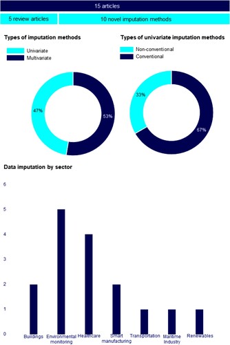
Data imputation techniques are divided into univariate and multivariate methods. Univariate approaches impute values of a parameter by only analysing its instances. Conversely, multivariate methods impute values of a parameter by the consideration of predictors, which are parameters that correlate with the response. The number of studies that contributed to the analysis of multivariate imputation techniques are nearly equal to the ones that considered univariate imputation techniques, as of the total of 32 machine learning and time series forecasting models implemented, 53% referred to univariate imputation techniques and 47% to the multivariate imputation methods. However, only one third of the presented univariate imputation methods were novel imputation algorithms, and thus the majority of the univariate imputation techniques implemented were conventional imputation approaches, such as vertical imputation and Last Observation Carried Forward (LOCF) models. Although these conventional methods were easy to interpret and implement, they presented major limitations that needed to be considered, such as the distortion of the parameter and the disruption of the relationship between the predictors and the response variable when implementing mean imputation and the statistical deficiencies of the LOCF model (Lachin 2016). Hence, further research on this basis needs to be accomplished. There are a number of studies demonstrating the efficient performance of time series algorithms, which are being used as forecasting approaches, when imputing missing values. For instance, Liu et al. (2020) implemented a technique named Itr-MS-STLDecImp based on the Seasonal and Trend decomposition using LOESS (STL) algorithm, which tried to predict the incomplete values by implementing pattern discovery, and thus decomposing the time series into trend, seasonal, and remainder components. Itr-MS-STLDecImp was utilised to recover large gaps of missing data. Also, Bokde et al. (2018) introduced an adjustment of the Pattern Sequence Forecasting (PSF) algorithm which incorporated control structures to assess characteristics that were repeated along the time series. This algorithm was referred to as imputePSF and was utilised to impute missing values in traffic speed time series from a loop detector, in time series of water flow rates generated from hydraulic simulations, and in a twenty-year time series of the monthly average air temperature at Nottingham Castle, England. Nonetheless, none of the studies proposed the utilisation of these approaches in conjunction with a multivariate imputation method to evaluate if the imputation is enhanced when it is performed by the consideration of incomplete predictors’ datasets. Furthermore, there is no evidence of any study that presents a novel univariate imputation method to deal with the missing data from time series sensor data of marine machinery systems. In this regard, only one study has been identified in this sector, in which the implementation of k-NN model in conjunction with the MICE method was considered to impute missing values (Cheliotis et al. 2019). However, both imputation techniques are multivariate methods, and thus predictors are required to complete the instances of a parameter. If there are no predictors available the mean imputation implemented in the MICE method can be considered as a final imputation technique, but, as discussed, due to the limitations of this approach the application of non-conventional univariate imputation techniques is recommended.

Multivariate imputation was mainly performed by machine learning methods, such as k-Nearest Neighbors (k-NN) and Support Vector Regressors (SVRs). For example, Ching et al. (2016) implemented a comparative study of five imputation methods (linear regression, weighted k-NN, SVM, mean imputation, and replacing incomplete values with zero). The different models were evaluated by using time series sensor data of a community centre floor. Linear regression yielded better accuracy when there was a linear relationship between the outcome and the predictors, whereas the implementation of SVM was suggested when the relation between features was nonlinear. Also, Izonin et al. (2019) introduced an imputation method based on the utilisation of the Ito decomposition and the AdaBoost algorithm. It was concluded that the proposed approach led to more accurate results than other analysed techniques, such as SVR and SGD regressor. Although the analysed multivariate imputation techniques led to accurate results, none of the studies contemplated the unavailability of predictors. Furthermore, each model presented various limitations that need to be considered when modelling the data imputation framework.

3. Methodology

Having critically observed the current literature, this paper suggests a novel method which brings together a number of features. These are related to the unavailability or incompleteness of the predictors’ dataset, which are addressed by the implementation of the first-order Markov chain as a univariate imputation technique. Also, the lack of analysis and formalisation of a data imputation framework in the maritime industry is tackled by presenting a novel data imputation approach that can be introduced in a holistic predictive framework. Furthermore, a comparative methodology is implemented as a multivariate imputation method to provide a general data imputation approach, which is presented in this paper. A graphical representation of this framework is expressed in Figure 2.

Figure 2. General framework for data imputation of marine systems sensor data.

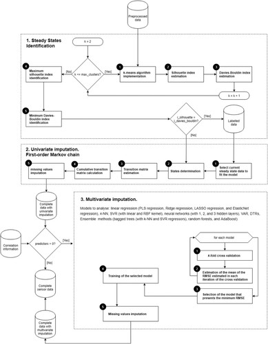
As the dataset may not only include steady operational states, both manoeuvring and transient states of machinery need to be identified and then discarded. Also, the data is standardised to ensure that all features contribute equally. Once the data preparation is completed, the dataset is available to be used as an input of the proposed framework, and thus the first step is implemented. This is the steady states identification, which applies the k-means clustering technique to identify the different steady states that the time series contains. To validate the clusters considered as the most appropriate, two validity indices are estimated (Silhouette and the Davies-Bouldin indices). Although another criterion can be implemented to select the optimal number of clusters, such as the inertia, these two indices provide more evident results. If the steady states identification is converged, the preceding values of the current steady state, identified after an instance with a missing value is detected, are used to implement the univariate imputation of the predictor's instance. Otherwise, the entire preceding values are used as an input to implement the second step, even though the preceding values do not correspond to the current steady state. Once the values fitting the univariate imputation model have been determined, the univariate imputation step is applied by the implementation of the first-order Markov chain, which considers that each subsequent state hinges only on the preceding state. This model is applied until all instances of each predictor are completed. Hence, as the predictors no longer contain missing values, the multivariate imputation step can be applied, which consists of the analysis of a total of 16 machine learning and time series forecasting models.

3.1. Steady states identification

Time series data of marine machinery parameters, such as the main engine power and the main engine rotational speed, may present steady states that are initiated after an abrupt change and persist over a certain period of time before another adjustment occurs. These abrupt changes refer to either weather conditions or to small adjustments that are applied due to the contractual agreements between the charterer and the shipowner in relation to the vessel speed and the fuel oil consumption per day.

Clustering is a widely used technique implemented to identify substantial groups of data. The records of each group are analogous to one another, but differ significantly with the ones clustered in the other groups. Hence, clustering can be applied to divide the time series automatically into the different steady states perceived in the sample. Then, when a missing value is detected, the current cluster is selected to be used as a feature to implement the first-order Markov chain. Among all the clustering techniques, the k-means clustering is utilised in this study due to its simplicity and scalability. One of the major limitations of this algorithm is the selection of the optimal number of clusters. Consequently, both the Silhouette (Starczewski and Krzyżak 2015) and Davies-Boulding indices are applied to select the most appropriate number of clusters.

3.2. Univariate imputation. First-order Markov chain

Once the steady states are identified, the univariate imputation is performed. Univariate techniques impute values of a feature by only considering the feature being analysed. By contrast, multivariate methods impute values of a feature by considering other features that are correlated with the feature being analysed. Thus, to apply any multivariate method, the completeness of the predictors’ dataset needs to be guaranteed. For this reason, the univariate imputation step is implemented prior to the multivariate imputation step to impute the missing values that the predictors of a feature may contain.

For that purpose, first-order Markov chain model, which considers that each subsequent state hinges only on the preceding state, is applied in this inquiry to assess its effectiveness when imputing missing values of sensor data of marine systems. Several approaches have been applied to produce synthetic data by implementing first-order Markov chain (Sahin and Sen 2001; Shamshad et al. 2005; Ching et al. 2006; Lawler 2006; Privault 2013; Pesch et al. 2015), although these methodologies have not been performed to impute missing values within the maritime industry to the best of the authors’ knowledge. Such approaches have been adapted to consider the different steady states and to perform univariate data imputation. The procedure is presented hereunder.

1. A collection of occurrences, $x_t$, indexed by time, are considered to identify, and impute missing values. It is determined that the occurrence at time $t$ just hinges on the previous value and not on all values at times before $t$. Such a conception is known as discrete time stochastic process, and more precisely Markov process. Thus, the time series values need to be clustered in a finite number of states so that the first-order Markov chain transition matrix can be estimated. To determine these states, Equation (1) is used. (1) $S_T=\overline{X}\pm ks$(1) where $S_T$ is the state determined, $\overline{X}$ is the mean, and $ks$ is $k$ standard deviations, $s$, which is added or subtracted until the maximum and the minimum values of the current state are achieved.

2. A discrete time stochastic process, $(X_n{)}_{n\in \mathbb{N}}$, which takes values in a finite set $S$, is considered to have the Markov property if the probability distribution of $X_{n+1}$ at time $n+1$ only hinges on the previous state $X_n$ at time $n$, and not on all the past values of $X_k$ for $k\le n-1$. Thus, (2) $\begin{array}{rl}& \mathbb{P}(X_{n+1}=j|X_n=i_n,X_{n-1}=i_{n-1},\dots ,Z_0=i_0)\\ & =\mathbb{P}(Z_{n+1}=j|Z_n=i_n)=p(i,j)\end{array}$(2) where $i_0,i_1,\dots ,i_n,j\in S$. The probability $p(i,j)$ indicates the probability that the previous state $i$ is followed by the current state $j$. All the possible transition probabilities of a process can be collected in a $rxr$ matrix, where each $(i,j)$ entry $P_{ij}$ is $p(i,j)$, (3) $\mathit{P}=(P_{ij}{)}_{1\le i,j\le r}=\left(\begin{array}{ccc}{p}_{1,1}& p_{1,2}& \begin{array}{cc}\cdots & p_{1,r}\end{array}\\ p_{2,1}& p_{2,2}& \begin{array}{cc}\cdots & p_{2,r}\end{array}\\ \begin{array}{c}⋮\\ p_{r,1}\end{array}& \begin{array}{c}⋮\\ p_{r,2}\end{array}& \begin{array}{cc}\begin{array}{c}\ddots \\ \cdots \end{array}& \begin{array}{c}⋮\\ p_{r,r}\end{array}\end{array}\end{array}\right)$(3) and that satisfies (4) $0\le P_{ij}\le 1,1\le i,j\le r,$(4) (5) $\sum _{j=1}^r{P}_{ij}=1,1\le i\le r.$(5)

3. The cumulative probability transition matrix needs to be encountered by using Equation (6) so that the data imputation process can be applied. (6) $P_{ir}=\sum _{j=1}^r{P}_{ij}$(6)

4. The following procedure is applied to impute missing values:

   1. The preceding state is considered as the initial state.

   2. By using a uniform random number generator, a random value, $\xi$, which varies between 0 and 1, is established.

   3. The $\xi$ value achieved is compared with the elements of the current state row of the cumulative probability transition matrix. Thus, if $\xi$ is higher than the cumulative probability of the preceding state but lesser than or equal to the cumulative probability of the successive state the new state is adopted.

   4. Finally, the missing values are imputed by using Equation (7). (7) $V=V_{\min }+\xi (V_{\max }-V_{\min })$(7)

This procedure is repeated for each steady state identified until all the missing values have been imputed.

3.3. Multivariate imputation

After the first-order Markov chain model is generated for every instance of each predictor that contains a missing value to impute, the predictors’ dataset is completed. Thus, the multivariate imputation step can be applied to impute the missing values of that feature. To that end, a comparative study is performed to assess the accuracy of a total of 16 machine learning and time series forecasting models. These models include: linear regression (Partial Least Squares regression, LASSO regression, Ridge regression, and ElasticNet regression), k-Nearest Neighbors, Support Vector Machines for Regression (with linear and RBF kernel), Neural Networks (with 1, 2, and 3 hidden layers), Vector Autoregressions (VAR), Decision Tree Regressors, and ensemble methods (Bagged Trees (with SVR and k-NN regressors), Random Forests, and AdaBoost). The accuracy of each model is assessed by estimating the Root Mean Square Error (RMSE). The model that presents the minimum RMSE value after the validation process implemented by applying the k-fold cross-validation technique is selected to train the model and, finally, impute the missing values. The models described in this section are an adaptation of the comparative study performed by Velasco-Gallego and Lazakis (2020).

The first family of machine learning models considered in this study are the linear regression models. This includes PLS regression, Ridge regression, LASSO regression, and ElasticNet regression. Linear regression models describe the relationship between a response feature and one or more explanatory features to predict the values of the response based on the explanatory features’ values. To obtain the best adjusted regression line, the Ordinary Least Squares (OLS) regression is implemented. OLS estimates the regression line that minimises the sum of squared residual values. One major limitation of this statistical method is that the solution provided by OLS may imply both high variability and instability if the predictors utilised in the multiple linear regression are strongly correlated. In such cases, the Partial Least Squares (PLS) is suggested. PLS explores linear combinations between the explanatory features, also referred to as components. These components are selected to both summarise the variation of the explanatory features at maximum and guarantee that the estimated components show maximum correlation with the response feature. Therefore, PLS is performed prior to the linear regression model if the explanatory features present high correlation. This collinearity can also be addressed with biased models. These biased regression methods are modelled by adding a penalty that regularises the parameter estimates to the sum of the squared error. Ridge regression considers the addition of a second-order penalty on the parameter estimates, whereas the Least Absolute Shrinkage and Selection Operator (LASSO) model adds a first-order penalty instead. An extended version of Ridge and LASSO regression models is the ElasticNet regression technique, which combines the two preceding penalties.

Also, non-linear regression models are also considered in this study, an example of which is the k-Nearest Neighbors (k-NN). k-NN aims to predict the missing values by considering k-closest records from the training set. Another widely implemented non-linear regression model considered in the study is the Support Vector Regressors (SVRs), which is formed by only those data points, the residuals of which present an absolute difference greater than a given threshold. The prediction function of the model in this inquiry is characterised by the application of both the linear and the Radial Basis Function (RBF) kernels. Neural Networks (NNs) are another example of non-linear regression methods. In this study, the Multi-Layer Perceptron (MLP) regressor is considered. In this inquiry the MLP regressors are modelled with 1, 2, and 3 hidden layers.

Regarding the time series forecasting techniques, only the Vector Autoregression (VAR) model is implemented, which is a generalisation of the univariate autoregressive model. VAR model considers bi-directional relationships between features, and thus it can predict a vector of time series iteratively by generating predictions for each feature included in the model.

The study is completed by the implementation of Decision Tree Regressors (DTRs) and ensemble methods. The basis of the prediction of DTRs is established by partitioning the feature space into subspaces in an iterative manner. One major limitation of this model is that the implementation of only one regression tree may lead to sub-optimal predictive performance due to, for instance, its instability. For this reason, ensemble methods are suggested. The Bootstrap Aggregation Tree, also referred to as Bagged Tree, is an example of an ensemble method. This ensemble method implements Bootstrapping in tandem with a regression model. Another example of an ensemble method is the Random Forest. This ensemble method adds randomness into the learning process, and thus it reduces correlation among predictors. In addition, Boosting methods are also analysed. The recursive modelling of composition is the basis of this type of ensemble methods. Thus, each consecutive model learns by considering the error information determined in the preceding iteration. An example of a boosting method is the adaptive boosting technique, also referred to as AdaBoost. AdaBoost performs weight adjustment procedures established by the errors of the ongoing predictions. Hence, in each iteration, more complicated predictions are identified to assign larger weights to them so that it can be targeted in more detail in the consecutive tree.

To implement the machine learning and time series forecasting models considered in this step the Python libraries Scikit-Learn (Pedregosa et al. 2011) and Statsmodel (Seabold and Perktold 2010) are utilised. Root Mean Square Error (RMSE) is utilised as a basis for comparing the efficiency of the various models applied. This is a type of scale-dependent error, and thus the estimated errors are on the same scale as the observations. Its value is obtained by estimating the squared root of the average of the squares of the residuals (Equation 8). (8) $\mathrm{RMSE}=\sqrt{{\displaystyle \frac{1}{n}\sum _{i=1}^n{(y_i-{\hat{y}}_i)}^2}}$(8)

4. Case study application and results

To determine the efficient performance of the proposed framework a DMD-MAN B&W 6S50MC-C main propulsion engine of a cargo vessel is analysed. Specifically, a total of four parameters are studied including the main engine rotational speed, the main engine power, the main engine fuel flow rate, and the scavenging air pressure of the scavenge air receiver.

Prior to the implementation of the data imputation framework, both manoeuvring and transient states of machinery are identified and discarded. Thus, a total of approximately 2160 instances of operational time series data collected with a one-minute frequency are considered for analysis. Standardisation is also applied.

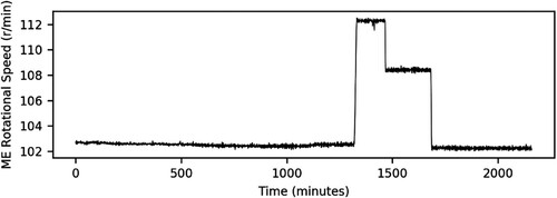
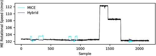
Figure 3 visualises the evolution of the main engine rotational speed time series. A total of four steady states are identified. The first steady state initiates at the first instant and persist around 103 rev/min over 1250 min. Then, an abrupt adjustment occurs and the rotational speed increases to over 112 rev/min. This state remains for roughly 130 min, and suddenly a slight adjustment occurs where the rotational speed decreases to approximately 108 rev/min. This third state lasts for around 215 min, and subsequently a last adjustment is perceived where the rotational speed decreases until it accomplishes the values observed in the first steady state. All noted adjustments refer to arrangements implemented due to the contractual agreements between the charterer and the shipowner where the vessel speed and the fuel oil consumption per day are defined.

Figure 3. Time series plot of the main engine rotational speed.

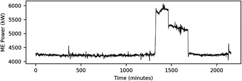
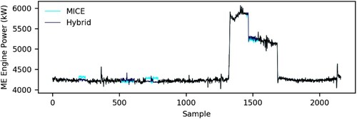
The main engine power indicates a similar progression. However, a higher variability can be observed, although it is still considered as low (Figure 4).

Figure 4. Time series plot of the main engine power.

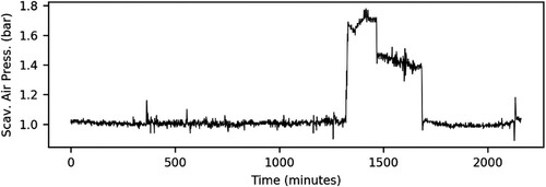
Correspondingly, the time series plots of both the main engine fuel flow rate and the scavenging air pressure of the scavenge air receiver system (Figures 5 and 6) present similar evolutions.

Figure 5. Time series plot of the main engine fuel flow rate.

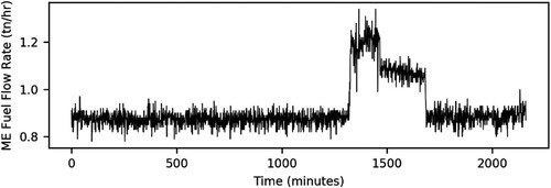
Figure 6. Time series plot of the main engine fuel flow rate.

Hence, as indicated in the Pearson's correlation coefficient matrix represented in Table 1, all four parameters are correlated between each other, as both the main engine fuel flow rate and the scavenging air pressure of the scavenge air receiver system are involved in the internal combustion process. This internal combustion process produces the linear movement of the piston, which promotes the rotational movement of the crankshaft to generate power.

Table 1. Pearson’s correlation coefficient matrix.

	ME rotational speed (rev/min)	ME power (kW)	ME fuel flow rate (tn/hr)	Scav. air pressure (bar)
ME rotational speed (rev/min)		0.99	0.95	0.99
ME power (kW)	0.99		0.96	1.00
ME fuel flow rate (tn/hr)	0.95	0.96		0.96
Scav. air pressure (bar)	0.99	1.00	0.96

To assess the performance efficiency of the proposed framework, samples of time series sensor data of marine machinery that present large gaps of missing values are analysed. To that end, a total of 5 large gaps of missing values are generated at random in each time series. The dimensions of these gaps are also defined randomly by selecting the dimension values between two thresholds. For this inquiry, the minimum and maximum number of missing values possible in each gap are set to 50 and 100, respectively.

In addition, for validation purposes, the performance of the proposed framework is compared with one of the most widely implemented imputation techniques, the Multivariate Imputation by Chained Equations (MICE), as presented in Cheliotis et al. (2019).

Figure 7 refers to the imputed time series of the main engine rotational speed parameter. In this case, all the gaps are located in the first steady state, with the exception of one that is detected in the last steady state of the time series. Both MICE and the proposed approach present similar results when imputing the gap located in the last steady state. However, it can be observed that the proposed methodology presents slightly better results than MICE, as the MLP regressor was identified as the most appropriate model to impute the missing values in this time series. Nonetheless, the imputation performances of both techniques differ significantly in the remaining gaps, as other parameters that are applied as predictors contain missing values at exactly the same timestamps. For instance, the fourth missing gap identified in the main engine rotational speed parameter is placed directly before minute 1000, as is the case of the main engine fuel flow rate and the scavenging air pressure of the scavenge air receiver. Thus, as the univariate imputation needs to be performed and both approaches apply different models, the difference in their respective performances are originated. Specifically, a percentage of improvement of 77% is accomplished in relation to the MICE approach when the proposed framework is implemented. These first results demonstrate the efficiency of the first-order Markov chain model as an imputation method against the mean imputation, which disrupts the relationships between variables. Also, the importance of preventing possible sensor failures that may derive in the collection of missing values can be perceived.

Figure 7. Large gaps imputation of the main engine rotational speed (This figure is available in colour online.).

Likewise, a similar pattern is represented in the imputation of large gaps of missing values from the main engine power. However, in this case the difference is not as significant. For example, as observed in Figure 8, two consecutive gaps are placed between the end of the second steady state and the start of the third steady state. It can be perceived for these states that there are no significant differences between the performance of the two approaches, as their predictors’ instances for these timestamps are completed and the multivariate model considered as the most appropriate for imputation in the proposed method is equivalent to the one applied in MICE, which is the multiple linear regression. By contrast, their performances differ when considering the first and third gap due to the incompleteness of the predictors’ instances for these timestamps. For this reason, the proposed framework leads to an improvement percentage of 56%.

Figure 8. Large gaps imputation of the main engine power (This figure is available in colour online.).

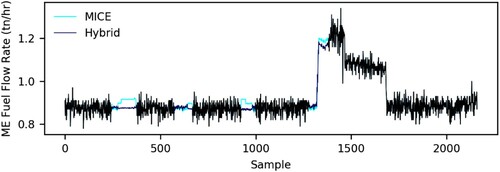
This pattern is again observed in the imputations implemented in the main engine fuel flow rate parameter (Figure 9). However, it can be noted that, although the predictors’ instances are completed for the timestamps where the last missing gap of this parameter is presented, there is a notable difference between the methods performance. This difference occurs due to the multivariate models implemented, as the model selected by the proposed framework is the LASSO regression. Hence, although multiple linear regression presents good results in this case, it can be demonstrated that other methods, which are not implemented by MICE, may lead to better results.

Figure 9. Large gaps imputation of the main engine fuel flow rate (This figure is available in colour online.).

The second highest percentage of improvement is identified in the scavenging air pressure of the scavenge air receiver parameter. The hybrid method proposed presents an improvement percentage of 73% in relation to the MICE method, even though the same multivariate model is applied in both techniques (Figure 10, Table 2).

Figure 10. Large gaps imputation of the scavenging air pressure of the scavenge air receiver (This figure is available in colour online.).

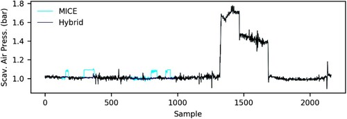
Table 2. Large gaps of missing values imputation results.

	RMSE
	Proposed framework	MICE	Percentage of improvement
ME rotational speed (rev/min)	0.17	0.75	77%
ME power (kW)	29.48	67.41	56%
ME fuel flow rate (tn/hr)	0.03	0.04	21%
Scav. air pressure (bar)	0.02	0.06	73%

Therefore, the proposed framework deals with some of the challenges derived from the application of IIoT. These challenges include the unavailability or incompleteness of the predictors’ dataset and the lack of analysis and formalisation of a data imputation framework in the maritime industry. Also, although the study presented only deals with large gaps of missing data, it can also be implemented to impute missing values that are missing completely at random. The major findings of the conducted study are expressed hereunder.

• The proposed hybrid framework outperforms the MICE approach when dealing with large gaps of missing values of time series sensor data of marine machinery systems.

• The mean imputation, which is utilised in the MICE approach, presents important limitations that need to be considered, such as the distortion of the parameter distribution and the disruption of the relationship between features, as these limitations derive in an increase of the imputation error. Thus, the first-order Markov chain model is suggested, as it leads to better results.

• The importance of the completeness of the dataset to avoid leading to poor data-driven models that assist decision-making processes.

• The influence of the appropriate selection of the multivariate model by the consideration of the characteristics of the dataset.

5. Conclusions

The maritime industry currently offers state-of-the-art maintenance and inspection processes. An example of which is condition-based maintenance (CBM), which is a maintenance strategy established by the monitoring of the assets’ conditions to decrease the number of failures associated with machinery. To facilitate this strategy, Industrial Internet of Things (IIoT) is applied so that a large number of sensors can be installed both alongside the most critical components and around the environment where these assets are operating. Despite the indisputable benefits that the implementation of this technology generates in the maritime industry, it presents several challenges, such as the collection of incomplete values due to certain errors. Also, it has been perceived that there is a lack of analysis and formalisation of a data imputation framework in the maritime industry.

Therefore, a novel framework is proposed to provide an approach that encompasses the imputation of large gaps of missing values from time series sensor data of marine machinery systems. This framework implements the univariate imputation by the application of the first-order Markov chain in tandem with a multivariate imputation approach based on a comparative study of a total of 16 machine learning and time series forecasting models. Among all the models included in the methodology, the most appropriate multivariate model is selected based on a validation process, which is constituted by the k-fold cross-validation technique.

The proposed framework is assessed by the implementation of a case study on a total of 4 parameters, obtained from sensors installed on the marine machinery systems of a cargo vessel, which presents large gaps of missing values. These parameters refer to the main engine rotational speed, the main engine power, the main engine fuel flow rate, and the scavenging air pressure of the scavenge air receiver. The hybrid approach outperforms the MICE method, obtaining the highest improvement percentage with a value of 77% when imputing the missing gaps from the main engine rotational speed. Therefore, the study conducted demonstrates the importance of the completeness of the dataset to avoid leading to poor data-driven models that assist decision-making processes. However, if this can not be guaranteed, the appropriate selection of the imputation models is indispensable to ensure the avoidance of bias in the estimates, as it is observed with the application of the first-order Markov chain, which leads to better results than the mean imputation due to its major limitations.

Hence, data imputation is a crucial step when utilising IIoT sensor data, and thus further research is needed to be addressed. Some future work guidelines considered are:

• The implementation of a comparative methodology, similar to the one implemented in the multivariate imputation step, as a univariate imputation approach where higher-order Markov chains are analysed.

• The addition of other metrics in the validation process, rather than the RMSE, to evaluate such aspects as the computational cost. Although the execution time has not been addressed in this study, as all models presented similar results in this aspect and the execution time of the proposed approach is the order of seconds, it can be critical when dealing with larger datasets.

• The analysis of optimisation algorithms for tuning hyperparameters.

• The implementation of deep learning algorithms as imputation techniques.

• The development of a real-time imputation technique to address instant data-driven decision-making processes.

• The prevention of incomplete data recording by the application of a monitoring and alerting tool.

Disclosure statement

No potential conflict of interest was reported by the author(s).

References

- Aheleroff S, Xu X, Lu Y, Aristizabal M, Velásquez JP, Joa B, Valencia Y. 2020. IoT-enabled smart appliances under industry 4.0: A case study. Adv Eng Inf. 43:1–14. doi:https://doi.org/10.1016/j.aei.2020.101043.
- Azimi I, Pahikkala T, Rahmani AM, Niela-Vilén H, Axelin A, Liljeberg P. 2019. Missing data resilient decision-making for healthcare IoT through personalization: A case study on maternal health. Future Gener Comput Syst. 96:297–308. doi:https://doi.org/10.1016/j.future.2019.02.015.
- Balakrishnan SM, Sangaiah AK. 2018. Chapter 6 – aspect oriented modeling of missing data imputation for Internet of Things (IoT) based healthcare infrastructure. Intelligent Data-Centric. 135–145. doi:https://doi.org/10.1016/B978-0-12-813314-9.00006-2.
- Bashir F, Wei H. 2018. Handling missing data in multivariate time series using a vector autoregressive model-imputation (VAR-IM) algorithm. Neurocomputing. 276:23–30. doi https://doi.org/10.1016/j.neucom.2017.03.097.
- Bokde N, Beck MW, Martínez Álvarez F, Kulat K. 2018. A novel imputation methodology for time series based on pattern sequence forecasting. Pattern Recognit Lett. 116:88–96. doi:10.1016/j.patrec.2018.09.020.
- Cheliotis M, Gkerekos C, Lazakis I, Theotokatos G. 2019. A novel data condition and performance hybrid imputation method for energy efficient operations of marine systems. Ocean Eng. 188:1–14. doi:10.1016/j.oceaneng.2019.106220.
- Ching W, Huang X, Ng M, Siu T. 2006. Markov chains. Models, algorithms and applications. 2nd ed. Singapore: Springer; p. 1–19.
- European Maritime Safety Agency (EMSA). 2020. Preliminary annual overview of marine casualties and incidents 2014-2019, URL: http://www.emsa.europa.eu/accident-investigation-publications/annual-overview.html.
- Eurostat. 2019. Energy, transport and environment statistics. Luxembourg: Publications Office of the European Union. https://ec.europa.eu/eurostat/en/web/products-statistical-books/-/KS-DK-19-001.
- Fekade B, Maksymyuk T, Kyryk M, Jo M. 2018. Probabilistic recovery of incomplete sensed data in IoT. IEEE Internet Things J. 5:2282–2292. https://ieeexplore.ieee.org/document/7987674.
- Hadeed SJ, O'Rourke MK, Burgess JL, Harris RB, Canales AR. 2020. Imputation methods for addressing missing data in short-term monitoring of air pollutants. Sci Total Environ. 730:1–7. doi:https://doi.org/10.1016/j.scitotenv.2020.139140.
- Izonin I, Kryvinska N, Tkachenko R, Zub K. 2019. An approach towards missing data recovery within IoT smart system. Procedia Comput Sci. 155:11–18. doi:https://doi.org/10.1016/j.procs.2019.08.006.
- Lachin JM. 2016. Fallacies of last observation carried forward analyses. Clin Trials. 13(2):161–168. doi:https://doi.org/10.1177/1740774515602688.
- Lawler G. 2006. Introduction to stochastic processes. 2nd ed. Boca Raton: Taylor & Francis Group, LLC; p. 1–12.
- Lazakis I, Dikis K, Michala AL, Theotokatos G. 2016. Advanced ship systems condition monitoring for enhanced inspection, maintenance and decision making in ship operations. Transportation Research Procedia. 14:1679–1688. doi:https://doi.org/10.1016/j.trpro.2016.05.133.
- Lazakis I, Gkerekos C, Theotokatos G. 2019. Investigating an SVM-driven, one-class approach to estimating ship systems condition. Ships Offsh Struct. 14:432–441. doi:https://doi.org/10.1080/17445302.2018.1500189.
- Liu Y, Dillon T, Yu W, Rahayu W, Mosafa F. 2020. Missing value imputation for industrial IoT sensor data with large gaps. IEEE Internet Things J. https://ieeexplore.ieee.org/abstract/document/8976165.
- Noor NM, Abdullah MMAB, Yahaya AS, Ramli NA. 2014. Comparison of linear interpolation method and mean method to replace the missing values in environmental dataset. Mater Sci. 803:278–281. https://www.scientific.net/MSF.803.278.
- Pedregosa F, et al. 2011. Scikit-learn: machine learning in Python. JMLR 12:2825–2830. https://jmlr.csail.mit.edu/papers/v12/pedregosa11a.html.
- Pesch T, Schröders S, Allelein H, Hake J. 2015. A new markov-chain-related statistical approach for modelling synthetic wind power time series. New J Phys. 17:1–15. http://iopscience.iop.org/article/10.1088/1367-2630/17/5/055001.
- Pratama I, Permanasari AE, Ardiyanto I, Indrayani R. 2016. A review of missing values handling methods on time series data. International Conference on Information Technology Systems and Innovation (ICITSI), pp. 1-6, url: https://ieeexplore.ieee.org/document/7858189.
- Privault N. 2013. Understanding Markov chains. Examples and applications. Singapore: Springer; p. 77–94.
- Priya Stella Mary I, Arockiam L. 2017. Imputing the missing data in IoT based on the spatial and temporal correlation. IEEE International Conference on Current Trends in Advanced Computing (ICCTAC), pp. 1-4, url: https://ieeexplore.ieee.org/document/8249990.
- Raptodimos Y, Lazakis I. 2018. Using artificial neural network-self-organising map for data clustering of marine engine condition monitoring applications. Ships Offsh Struct. 13:649–656. doi:https://doi.org/10.1080/17445302.2018.1443694.
- Raptodimos Y, Lazakis I. 2020. Application of NARX neural network for predicting marine engine performance parameters. Ships Offsh Struct. 15:443–452. doi:10.1080/17445302.2019.1661619.
- Sahin A, Sen Z. 2001. First-order Markov chain approach to wind speed modelling. J Wind Eng Ind Aerodyn. 89:263–269. doi:https://doi.org/10.1016/S0167-6105(00)00081-7.
- Seabold S, Perktold J. 2010. Statsmodels: econometric and statistical modeling with python. Proceedings of the 9th Python in Science Conference, pp. 92-96. https://conference.scipy.org/proceedings/scipy2010/pdfs/seabold.pdf.
- Shamshad A, Wan W, Bawadi M, Sanusi S. 2005. First and second order Markov chain models for synthetic Generation of wind speed time series. Energy. 5(30):1–21. doi:https://doi.org/10.1016/j.energy.2004.05.026.
- Starczewski A, Krzyżak A. 2015. Performance evaluation of the Silhouette index. Artificial Intelligence and Soft Computing. ICAISC 2015. Lecture Notes in Computer Science, vol 9120. Springer, Cham, doi: https://doi.org/10.1007/978-3-319-19369-4_5.
- Velasco-Gallego C, Lazakis I. 2020. Real-time data-driven missing data imputation for short-term sensor data of marine systems. A comparative study. Ocean Eng. 218:1–23. doi:https://doi.org/10.1016/j.oceaneng.2020.108261.