Bayesian and machine learning-based fault detection and diagnostics for marine applications

ABSTRACT

Marine maintenance can improve ship performance by leveraging predictive maintenance, Machine Learning and Data Analytics. This paper aims to enrich the literature, by developing a novel framework for ship diagnostics based on operational data and the probability of faults. Moreover, the framework can identify the root cause of developing faults avoiding black-box Neural Networks, and complex physics-based models. This research integrates Machine Learning-based Fault Detection, Exponentially Weighted Moving Average control charts, and Bayesian diagnostic networks which allow the examination of the rate of development (fault profile) of faults and failure modes. For validation, the case study of a marine Main Engine is used to examine faults in the engine’s Air Cooler and Air and Gas Handling System. It is concluded that any simultaneous abnormal deviations in the Main Engine’s Exhaust Gas Temperature are more likely to be caused by a fault in the Air and Gas Handling System.

KEYWORDS:

• Condition monitoring
• ship system diagnostics
• Bayesian networks
• fault detection
• machine learning
• ship safety

1. Introduction

Machinery Fault Detection (FD) and diagnostics are integral parts of modern predictive maintenance and they are used to provide accurate predictions for targeted maintenance (Kobbacy 2008; Mohanty 2015; Karatug and Arslanoglu 2020; Karvelis et al. 2021). As a result, FD and diagnostics have a positive impact on safety as discussed by Turan et al. (2009), Lazakis et al. (2010) and Dikis et al. (2015) and can be viewed as hazard mitigation tools (EMSA 2018).

There is substantial literature from many different sectors (e.g. offshore, nuclear) demonstrating the benefits (i.e. fast and accurate models) of regression-based Expected Behaviour (EB) modelling for FD. Zaher et al. (2009) used Artificial Neural Networks (ANN) in EB models for FD in the gearbox of a wind turbine based on operational data. Moreover, Schlechtingen and Santos (2014) compared the effectiveness of polynomial regression models and ANN in EB models for FD. Both types of models exhibited good performance in identifying faults in the stator and gearbox of a wind turbine. Likewise, Schlechtingen et al. (2013) used ANN for the detection of structural and mechanical faults in wind turbines. Bangalore and Patriksson (2018) used an ANN-based EB model for FD in critical components of wind turbines and for optimal maintenance planning. Similarly, the Exponential Weighted Moving Average (EWMA) has been deployed in a variety of cases for the detection of sensitive faults, filtering of noise and trend-checking (Isermann 2006; Garoudja et al. 2017). Harrou et al. (2015) used EWMA in an FD methodology for distillation columns. Moreover, Badodkar and Dwarakanath (2017) detected broken teeth in mechanical gearboxes, from their early onset, by smoothing acceleration signals with the EWMA. Also, Nounou et al. (2018) proposed an EWMA-based predictive maintenance scheme for photovoltaic panels using performance parameters (voltage, current, etc.). Lastly, Adegoke et al. (2019) developed an EWMA-based FD methodology for the manufacturing sector.

Diagnostic models can be categorised into (a) physics-based models, (b) data-driven models and (c) knowledge-based models (Jardine et al. 2006; McKee et al. 2014; Coraddu et al. 2021), based on their underlying algorithms. Under the scope of this work, knowledge-based models are examined due to their advantages. In detail, they have the distinct benefit of mimicking specialists’ reasoning while effectively handling uncertainties, and not resorting to time-consuming physics-based, or black-box ANN models (McKee et al. 2014). In general, knowledge-based models have many implementations, but the more prominent approaches are based on Bayesian Networks (BN) (Chojnacki et al. 2019; Wang et al. 2019).

Knowledge-based BN are extremely popular in diagnostic tasks due to their compact nature, consistency, and modularity (Cai et al. 2017; Babaleye and Kurt 2020). For instance, Riascos et al. (2007) used BN for the diagnosis of faults in a proton exchange membrane fuel cell. Also, Diakaki et al. (2015) developed a model for route optimisation and fault localisation based on BNs. Atoui et al. (2015) developed a BN-based classifier for the detection and diagnosis of faults in chemical process plants. Moreover, Zhao et al. (2017) created a BN for the diagnosis of more than 27 faults in industrial air handling units, demonstrating the versatility of BN, as they make use of data fusion. The versatility and accuracy of BNs are demonstrated in the work of Wang et al. (2017), through the development of a diagnostic network for chiller units. Ami et al (2018), looked at the development of dynamic BN for FD and root-cause analysis for chemical process plants, generating evidence for collected data under the assumption of a Gaussian distribution. The effectiveness of BNs for diagnostic tasks, and consequently improved safety, is demonstrated in numerous research efforts applied in different industries, but with limited applicability in the maritime (Riascos et al. 2007; Tantele and Onoufriou 2009; Atoui et al. 2015; Cai et al. 2016; Zhao et al. 2017).

The maritime industry is taking quick steps to benefit from the applications of machine learning and data analytics. There are many examples of machine learning applications tackling a plethora of issues ranging from fault detection to route optimisation (Lazakis et al. 2018; Raptodimos and Lazakis 2018; Iraklis Lazakis et al. 2019; Cheliotis et al. 2020; Tan et al. 2020). However, the application of modern diagnostic tools for shipboard systems is very limited and underdeveloped. For example, Silva et al. (2018) used two-dimensional wavelet transforms for the diagnosis of faults in the electrical system of a ship. Similarly, Campora et al. (2018) developed an ANN and a thermodynamic model for fault diagnostics of naval gas turbines. Moreover, Korczewski (2016) investigated the use of the Main Engine (ME) Exhaust Gas Temperature (EGT) in thermodynamic models for the diagnosis of engine internal faults. Homik (2010) used vibration signals in an FD and diagnostics methodology for torsional vibration dampers and marine ME crankshafts. Finally, Ranachowski and Bejger (2005) studied the use of wavelet analysis from acoustic signals for the diagnosis of common faults in the fuel injection systems of a marine diesel engine.

1.1. Comparison and gaps

From the previously cited literature, the following inferences regarding maritime diagnostics can be made. Overall, the size and quality of available datasets are not uniform as only sparse datasets are available for each ship application. Consequently, the algorithms included in the developed frameworks should be streamlined with these issues in mind.

It is observed that ANNs form the core of most EB models for FD. Despite their good performance, they require large datasets for training which are not readily available in the maritime industry. Also, ANNs are black-box approaches making it challenging to impart domain knowledge. The core approach for the EB model should serve the application and address the characteristics of the available data. In cases with sparse data and requirements for precise results, regression-based EB models should be considered.

Also, the use of EB models for FD is advantageous compared to the alternative classification approaches. With EB models there is greater flexibility in the selection of the underlying algorithms. In classification, in the absence of recorded faulty data one-class Support Vector Machines (SVM) are the standard choice, with few alternatives. Moreover, EB models are easier to integrate with diagnostic tasks.

In addition, most diagnostic models are physics-based which even though perform well they are time-consuming to develop. Likewise, data-driven diagnostic models also exhibit good behaviour, but they depend on large training datasets which are scarce in the maritime industry. On the contrary, knowledge-based diagnostics, including BNs, offer accurate performance without requiring lengthy set-up times or large amounts of training data. Furthermore, knowledge-based diagnostics are modular which improves their compatibility with FD modules and makes it easier to expand in other engineering systems.

From the above, it is inferred that the area of marine systems diagnostics is still under active development. Diagnostic efforts in the maritime field are very limited and cover only a few of the available systems. There is a gap for the development of a novel diagnostic framework that tackles the previously mentioned issues while benefiting from regression-based EB modelling, EWMA control chart, and BNs diagnostics and addressing the particular needs of maritime predictive maintenance. Also, there is a distinctive gap in the application of such a framework for ship propulsion plants.

1.2. Novelty and impact

The innovation of this work lies in the development of a novel framework that combines a machine learning based FD module with a BN-based diagnostic module. The FD module includes the pre-processing of data, multiple Polynomial Ridge Regression (PRR) for the development of an EB model, and EWMA control charts for the analysis of the residuals and the detection of faults. The FD module is combined in a novel way with the diagnostic module which includes the mapping of faults and the construction of a BN. Evidence of detected faults are propagated in a BN network. Then, the BN outputs quantified probabilities of the mapped faults together with the fault profiles of different failure modes.

By applying the novel diagnostic framework the maritime industry will benefit from (a) the ability to capture previously unseen faults based on the EB model, (b) the use of EWMA control charts to accurately detect developing faults (c) the ability to monitor real-time the development of faults and assess the condition of the selected system and (d) the practical and interoperable integration of FD with diagnostic tasks in a holistic novel framework catering to the needs of the maritime industry. Overall, the developed framework will allow the real-time detection and diagnosis of developing faults. This has a tangible impact on the effectiveness of maintenance planning and operational efficiency of ships. This will also enhance safety and reduce unavailability by creating time for pre-emptive actions. As seen, this novel framework can be used by ship operators to contribute to the safe and efficient operations of vessels.

In the rest of the paper, Section 2 discusses the details and novelty of the developed methodology, Section 3 presents the case study together with the results, and Section 4 provides the overall conclusions and future work.

2. Proposed methodology

The goal of this study is to establish a novel Bayesian and machine learning based diagnostic framework for practical ship system applications. To that end, machine learning tools are used for data pre-processing and the creation of an EB model. Subsequently, these are combined with EWMA control charts in a novel integration with fault mapping and BNs.

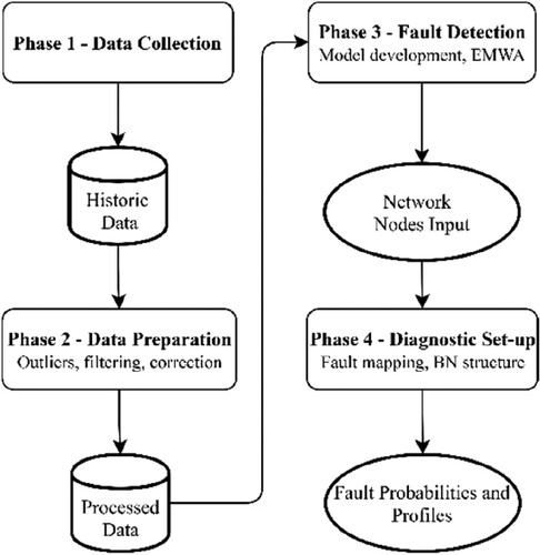
To fulfil the above, four interconnected phases are developed (Figure 1). These phases are:

1. Data collection: comprising of the data gathering efforts from a data acquisition system and other sources.

2. Data preparation: comprising of the pre-processing tasks, such as outlier detection, data filtering and correction to reference conditions

3. Fault detection: comprising of the development and application of the PRR model and EWMA control chart

4. Diagnostic Set-up: comprising of the pairing between monitored variables and corresponding faults and the creation of BN structure.

Figure 1. Developed methodology flowchart (This figure is available in colour online.).

2.1. Data collection

Data collection is the initiating phase of the methodology that outputs a database with historic data (Figure 1), which is used throughout the methodology. The gathered data originate from a commercial data acquisition system installed onboard a merchant vessel. Normally, data acquisition signals for FD and diagnostic tasks of engineering systems include performance parameters (power outputs, speeds, etc.). Moreover, the sampling frequency can range from one recording per second to one recording per five minutes.

2.2. Data preparation and pre-processing

Data preparation is the essential second phase of the methodology, which includes the pre-processing tasks necessary to prepare and enhance the gathered data for the next steps of the analysis, as discussed by, Tanasa and Trousse (2004), Kotsiantis et al. (2006) and Cheliotis et al. (2019). The processes of this phase are performed using the Python programming language, and its output is the transformation of the collected historic data into ‘cleaned’ processed inputs.

The data preparation phase initiates with form handling and units checking of the data and then proceeds with the use of the Density-Based Spatial Clustering of Application with Noise (DBSCAN) algorithm for outlier and transient-state detection and removal. Outliers are sparse data points with considerably dissimilar values caused by sensor errors and instrumentation faults. It should be clarified that outliers are not part of fault suggestive patterns. The DBSCAN algorithm is an effective tool for the identification of outliers and other ill-recorded information, as demonstrated by many studies (Chen and Li 2011; Çelik et al. 2011; Thang and Kim 2011). DBSCAN is a density-based spatial algorithm that examines each point in the dataset to identify dense areas of points (clusters). The clusters are defined by the minimum number of points required to form a cluster (minP) and the maximum distance between points for them to be considered in the same cluster ($ϵ$) (Chen and Li 2011; Çelik et al. 2011; Thang and Kim 2011). Finally, additional value-based data filtering takes place, which ensures that the data represent only operational periods and the remaining data are corrected to account for the environmental influences, as per standard practices (ISO 2008; MAN B&W 2014).

2.3. Fault detection

The FD phase follows the data preparation phase and includes the EB model and the EWMA control chart. An EB model is developed to predict the expected behaviour of a specified variable, based on certain inputs. Then, the output of the EB model is compared with incoming data of the variable to obtain the residuals. The residuals are finally analysed in the EWMA to detect any faults. Once the results from the fault detection phase are obtained, they are aggregated and used as input in the diagnostic set-up phase of the methodology.

2.3.1. EB model development

For the EB model, multiple PRR is used due to its accurate and reliable performance as reviewed by Olive (2005), Bowerman et al. (2015) and Cheliotis et al. (2020). The training, validation and testing performance of the model is carried using the $R^2$ metric. In general, the developed polynomial regression model for the specified variable has a form as shown in Equation (1). That equation represents the general form of zth order polynomial using two predictor variables ($x_1,x_2$), having $w_0$ to $w_p$ as the regression coefficients, $b$ is the axis intercept and $\hat{y}$ the prediction for the target (specified) variable. (1) $\hat{y}=w_0{x}_1+w_1{x}_2+w_2{x}_1{x}_2+\dots w_p{x}_1^z+w_p{x}_2^z+b$(1) From the available data, a segment is used for training and validating to fit and fine-tune the algorithm. During training sets of known predictor variables ($x_1,x_2$) together with target variables ($y$) are used as input in Equation (1) to get estimates for the regression coefficients and the axis intercept. The training proceeds with the minimisation of the objective function shown in Equation (2). The objective function of the ridge regression includes the term $a\Vert w{\Vert }_2^2$, which limits the magnitude of the regression coefficients to avoid overfitting. The user-specified hyperparameter, $\alpha$, is responsible for controlling the limiting amount of L2. For the determination of the optimum $\alpha$ value, k-fold cross-validation was used, as detailed in Müller and Guido (2015) and Cheliotis et al. (2020). (2) $\mathrm{R}\mathrm{i}\mathrm{d}\mathrm{g}\mathrm{e}:\Vert \hat{y}-y{\Vert }_2^2+a\Vert w{\Vert }_2^2\mathrm{w}\mathrm{i}\mathrm{t}\mathrm{h}a\in \left[0,\mathrm{\infty }\right)$(2) The general working process that is followed for the development of the EB model is shown in the following pseudocode (Algorithm 2.3.1). This algorithm requires as inputs the predictor and target variables. It also requires the number of folds for the k-fold cross-validation and the size of the test set. Lastly, the set of the considered values for the model’s hyperparameters is given. Algorithm 2.3.1 represents the generalised process for the development of a supervised model, including the optimisation of one of its hyperparameters.

Algorithm 2.3.1 (Cheliotis et al. 2020)

2.3.2. EWMA control chart

Once the EB model is developed it is used to obtain the residuals of the specified (target) variable, as seen in Equation (3). In Equation (3), $\widehat{y_k}$ represents the predicted value of the kth instance of the target variable and $y_k$ is the actual value of the kth instance of the target variable. (3) $\begin{array}{rl}& r_k=\widehat{y_k}-y_k\\ & \mathrm{f}\mathrm{o}\mathrm{r}k=1,\dots N\end{array}$(3) Using residuals for FD is a proven and effective strategy. By comparing the ideal value of a variable with the incoming data we can quantify any variations and classify them, given a set of operating conditions (Martinez-Guerra and Luis Mata-Machuca 2013; Harrou et al. 2015).

The residuals are then used to construct the EWMA control chart. Equation (4) calculates the EWMA statistic (q) for all of the $k$ instances of the target variable, with $q_0$ representing the mean value of the specified variable in the incoming data. The calculation of the EWMA statistic also requires $r_k$, together with the user-defined smoothing parameter, $\lambda$. In this paper, the smoothing parameter was given the value of 0.4 according to common practices and by following the suggestions of Badodkar and Dwarakanath (2017), and Cheliotis et al. (2020). (4) $\begin{array}{rl}& q_k=\lambda r_k+\left(1-\lambda \right)q_{k-1}\\ & \mathrm{f}\mathrm{o}\mathrm{r}k=1,\dots N\\ & \mathrm{a}\mathrm{n}\mathrm{d}\lambda \in \left(0,1\right]\end{array}$(4) Lastly, the Upper Control Limit (UCL) and Lower Control Limit (LCL) are calculated. These limits provide the basis for the detection of faults, as any point that exceeds them signify faults. In other words, the UCL and LCL form the envelope of normal operations for the selected variable. In Equations (5) and (6) the mean value of the specified variable in the incoming data (${\mu }_0$) and the standard deviation ($\sigma$) are used. Lastly, $L$ signifies the width of the control chart and is empirically given a value of 3. Since the value of $L$ affects the envelope of normal operations, it must be appropriately selected so that it can correctly classify normal operating points. As the recorded data represent ‘healthy’ operating points, the resulting envelope must fully enclose all the data points. (5) $\mathrm{U}\mathrm{C}\mathrm{L}={\mu }_0+L\sigma \sqrt{{\displaystyle \frac{\lambda }{2-\lambda }\left[1-{\left(1-\lambda \right)}^{2i}\right]}}$(5) (6) $\mathrm{L}\mathrm{C}\mathrm{L}={\mu }_0-L\sigma \sqrt{{\displaystyle \frac{\lambda }{2-\lambda }\left[1-{\left(1-\lambda \right)}^{2i}\right]}}$(6)

2.4. Diagnostic set-up

Diagnostic set-up is the next phase of the methodology and uses as input aggregated results from the fault detection. The goal is to use real-time information to produce accurate probabilities of different faults occurring in the system. For that purpose, this phase initiates with the fault mapping, which includes the pairing between monitored variables and corresponding faults; then, the structure of the diagnostic BN is determined.

2.4.1. Fault mapping

Fault mapping is a very important task as it identifies the potential faults that can be diagnosed in a selected system, and the variables required for their diagnosis. Alongside the required variables, the acceptable range and behaviour of each variable are specified. Lastly, any additional tests for the diagnosis of specific faults are determined. Fault mapping is based on domain knowledge and by taking into consideration the operating manuals of the selected systems, provided by the equipment’s manufacturer or operator.

2.4.2. Bayesian network

Once the pairing between monitored variables and corresponding faults is completed, the structure of the diagnostic BN is determined. The identified faults are represented in the primary and secondary fault nodes of the network, while the variables required for the monitoring are used in the observable nodes. Any additional tests required for the investigation of a fault are inserted in the test nodes. Lastly, any other nodes concerned with the inner workings of the diagnostic tool can be inserted in the control nodes section.

BNs represent a joint probability distribution of a set of random variables and consist of a qualitative part and a quantitative part. The qualitative part is defined by a probabilistic Directed Acyclic Graphical (DAG) model where each variable is depicted as a node and links between them define causal relationships. The quantitative part is defined by the conditional probability distribution in the Conditional Probability Table (CPT) of each node (Ruggeri et al. 2007). BNs are based on Baye’s theorem, and calculate the posterior conditional probability distribution of occurrence of a fault given some observable evidence, as shown in Equation (7) (Langseth and Portinale 2007; Horný 2014; Cai et al. 2017). In detail, the posterior conditional probability distribution of occurrence of a fault is calculated using the clustering inference algorithm based on the size of the network and its documented positive characteristics (Yu et al. 2004; Zheng et al. 2019). (7) $P\left(\mathrm{f}\mathrm{a}\mathrm{u}\mathrm{l}\mathrm{t}|\mathrm{e}\mathrm{v}\mathrm{i}\mathrm{d}\mathrm{e}\mathrm{n}\mathrm{c}\mathrm{e}\right)={\displaystyle \frac{P\left(\mathrm{f}\mathrm{a}\mathrm{u}\mathrm{l}\mathrm{t}\right)P\left(\mathrm{e}\mathrm{v}\mathrm{i}\mathrm{d}\mathrm{e}\mathrm{n}\mathrm{c}\mathrm{e}|\mathrm{f}\mathrm{a}\mathrm{u}\mathrm{l}\mathrm{t}\right)}{P\left(\mathrm{e}\mathrm{v}\mathrm{i}\mathrm{d}\mathrm{e}\mathrm{n}\mathrm{c}\mathrm{e}\right)}}$(7) Assuming a set ($U$) of $n$ random variables $U=\left(X_1,X_2,\dots X_j,\dots ,X_n\right)$, a BN with $n$-nodes can be constructed. Moreover, $X_j$ represents the jth variable. The BN for the $n$ variables can be represented by Equation (8), where $pa\left(X_j\right)$ denotes all the parent nodes of $X_j$. 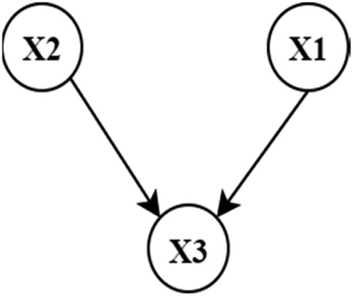(8) $P\left(X_1,\dots X_j,\dots ,X_n\right)=\prod _{j=1}^{n}P\left(X_j\right|pa\left(X_j\right))$(8) For example, the case of a simple network is considered in Figure 2, assuming that each variable has only two states, True ($t$) and False ($f$). Consequently, Equation (8) takes the form of Equation (9), by using the chain rule of probabilities and a conditional independence assumption. The conditional independence assumption dictates that a child node ($X_j$) is statistically dependent only to its parents $\left(pa\right(X_j\left)\right)$. (9) $P\left(X_1,X_2,X_3\right)=P\left(X_1\right)P\left(X_2\right)P\left(X_3\right|X_1,X_2)$(9) Therefore, the probability $P\left(X_3=t\right)$ is represented in Equation (10), which is also referred to as the prior probability of $X_3$. (10) $P\left(X_3=t\right)=P\left(X_3=t,X_1,X_2\right)=P\left(X_1\right)P\left(X_2\right)P(X_3=t|X_1,X_2)$(10) Also, assuming that $X_3$ is observed to be at its True state, then the probability of $X_2$ occurring $\left(P\right(X_2=t|X_3=t))$ can be found by using Equation (11). (11) $P\left(X_2=t|X_3=t\right)=P\left(X_2=t,X_1|X_3=t\right)={\displaystyle \frac{P\left(X_3=t|X_2=t,X_1\right)\ast P\left(X_2=t\right)}{P(X_3=t)}\ast P\left(X_1\right)}$(11) Equation (11) is also referred to as the posterior probability, and the first part of the product is due to Equation (7), while the second term is due to the joint probability distribution.

Figure 2. Sample BN with three nodes X1, X2, X3 (This figure is available in colour online.).

For this study, two types of evidence were used, namely hard evidence and virtual evidence. The former represents the traditional type of evidence used in BNs, which dictate the value or state of a variable (e.g. $X_1=\mathrm{T}\mathrm{r}\mathrm{u}\mathrm{e}$). In this paper, hard evidence was used for strict diagnostic tasks, to obtain the probabilities of examined faults based on monitored variables. However, hard evidence can introduce troublesome assumptions, especially when the value of a variable is very close to a state’s decision boundary. To counter this issue, and to extend the capabilities of the diagnostic network, virtual evidence was used. Virtual evidence represent evidence with uncertainty and was also used to obtain the fault profiles of the examined faults (Bilmes 2004; Korb and Nicholson 2010; Mrad et al. 2012). For instance, $X_1=0.7\mathrm{T}\mathrm{r}\mathrm{u}\mathrm{e}$ is considered as virtual evidence and represents that $X_1$ is almost in its true state.

3. Case-Study

3.1. Data collection

This section of the paper demonstrates the application of the developed methodology in a case study. The used data originate from a 65,000 DWT dry bulk carrier and were collected from the installed data acquisition system. The system has a 5-minute sampling rate and recordings during the first three months of 2017 were collected, resulting in 25’627 instances per variable.

For this paper, the ME of the ship and its supporting systems are studied (Figure 3). The ME EGT is selected for monitoring, as it can help uncover developing faults, both within the engine and in the supporting systems. In detail, faults in the air cooler, turbocharger and gas passages of the ME can manifest through changes in the ME EGT (MAN B&W 2017; Zhan et al. 2007; Woodyard 2009). Lastly, Table 1 shows the collected variables together with a description and their diagnostic purpose.

Figure 3. ME system representation (This figure is available in colour online.).

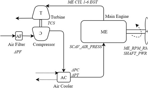
Table 1. Information for the used variables.

Variable Name	Description	Units	System	Role
ME CYL 1 EGT	ME cylinder 1 EG temperature	^oC	Main Engine (ME)	Monitored (target) variable
ME CYL 2 EGT	ME cylinder 2 EG temperature	^oC	Main Engine (ME)	Monitored (target) variable
ME CYL 3 EGT	ME cylinder 3 EG temperature	^oC	Main Engine (ME)	Monitored (target) variable
ME CYL 4 EGT	ME cylinder 4 EG temperature	^oC	Main Engine (ME)	Monitored (target) variable
ME CYL 5 EGT	ME cylinder 5 EG temperature	^oC	Main Engine (ME)	Monitored (target) variable
ME_RPM_TM	ME shaft speed	RPM	Main Engine (ME)	Predictor Variable
SCAV_AIR_PRESS	ME scavenging air pressure	bar	Main Engine (ME)	Predictor Variable/Diagnostic Test
SHAFT_PWR	ME shaft power	kW	Main Engine (ME)	Diagnostic Test
ΔPC	Scavenging air pressure drop across air cooler	mmWC	Air Cooler (AC)	Diagnostic Test
ΔPT	The temperature difference between air cooler air outlet and air cooler water inlet	^oC	Air Cooler (AC)	Diagnostic Test
TCS	Turbocharger speed	RPM	Turbocharger (TC)	Diagnostic Test
ΔPF	Pressure drop across turbocharger air filter	mmWC	Air Filter (AF)	Diagnostic Test

3.2. Data preparation and pre-processing

Data preparation begins with form handling and units checking and continues with the application of the DBSCAN algorithm for outlier and transient detection. Lastly, the data are filtered, using a value-based approach, to ensure that they represent only operational periods. During this study, the user-defined hyperparameters $ϵ=0.23$ and $\mathrm{m}\mathrm{i}\mathrm{n}P=11$ are used for the application of the DBSCAN algorithm. The selected values of the $ϵ$ and $\mathrm{m}\mathrm{i}\mathrm{n}P$ hyperparameters were achieved after iterative attempts and according to Chen and Li (2011), Gaonkar and Sawant (2013), Rahmah and Sitanggang (2016) and Schubert et al. (2017). Finally, the remaining data are filtered according to Equation (12). 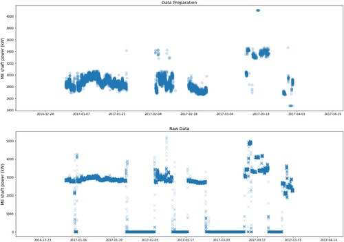(12) $\mathrm{P}\mathrm{o}\mathrm{w}\mathrm{e}{\mathrm{r}}_{\mathrm{M}\mathrm{a}\mathrm{i}\mathrm{n}\mathrm{E}\mathrm{n}\mathrm{g}\mathrm{i}\mathrm{n}\mathrm{e}}>5\mathrm{k}\mathrm{W}$(12) The application of the data preparation phase is demonstrated in Figure 4, showing the ME shaft power before (bottom chart), and after (top chart) the identification and filtering of the outliers and transient states. As can be observed, the data preparation phase can identify and remove sudden ‘spikes’, ‘dips’ and ‘flat-lines’ in the data.

Figure 4. Representative sample of the application of the data preparation phase in the ME shaft power showing the prepared data (top) and raw data (bottom) The y-axis of the top graph is scaled for clarity of the visualisation (This figure is available in colour online.).

3.3. Fault detection

3.3.1. EB model specification

From the data, 80% are used for training and validation, while the rest are kept for testing. For the process described in Algorithm 1, a five-fold cross-validation procedure is used. As a result, a fifth order multiple PRR model with $\alpha =0.6$ is obtained. Also, the ME scavenging air pressure and the ME shaft speed are used as predictor variables to obtain the ME EGT for each cylinder (target variable). The selection of the target variables was based on domain knowledge and after experts’ advice. In detail, the resulting model exhibits good training, validation and testing performance with$R_{\mathrm{T}\mathrm{R}\mathrm{A}\mathrm{I}\mathrm{N}\mathrm{I}\mathrm{N}\mathrm{G}}^2=0.92$, $R_{\mathrm{V}\mathrm{A}\mathrm{L}\mathrm{I}\mathrm{D}\mathrm{A}\mathrm{T}\mathrm{I}\mathrm{O}\mathrm{N}}^2=0.9$ and $R_{\mathrm{T}\mathrm{E}\mathrm{S}\mathrm{T}\mathrm{I}\mathrm{N}\mathrm{G}}^2=0.9$ respectively. In addition, the test set is used to ensure the multiple PRR model has good generalisation capabilities as it examines its performance in previously unseen data.

3.3.2. EWMA and verification

The FD phase concludes with the analysis of the residuals in an EWMA control chart. To evaluate the detection capabilities of the FD module, and by considering the fault-free nature of the used data, a sensitivity analysis is performed (Saltelli 2004; Law 2009). Since the collected data represent healthy operating conditions, as confirmed by the vessel’s operator, the EWMA control chart must not detect any faults.

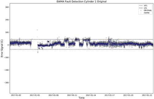
Figure 5 shows the performance of the EWMA-based FD chart, in an example for Cylinder 1. As can be seen, the FD module correctly avoids the detection of any faults, as the envelope of normal operations, defined by the ULC and LCL, is not exceeded.

Figure 5. EWMA control chart representing healthy operating points, in the indicative example of Cylinder 1 of the ME (This figure is available in colour online.).

To further evaluate the FD module, an artificial fault is introduced, and the FD module is tested on its capability to detect it. The use of artificial fault is necessary due to the fault-free nature of the used data, which is a very common problem in applications from merchant vessels (Cheliotis et al. 2020). The maritime industry can be reluctant in sharing performance and condition datasets, even more so when they contain faulty data. The artificial fault is introduced in terms of increased residuals, according to domain knowledge and by examining the publications of Hountalas (2000), and Theotokatos and Tzelepis (2015). This verifies that the simulated failure is amongst the predominant failure modes of the examined system. The increased residuals are caused by a gradual increase in the ME scavenging air pressure (predictor variable) until the alarm limit (3.30 bar) for the variable is exceeded. The alarm limit is specified by the ME manufacturer and is obtained from the ME’s operating manual (MAN B&W 2017).

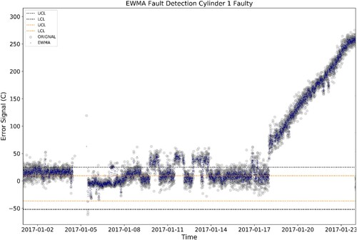
Figure 6 shows the performance of the FD chart in detecting the artificial fault, in an indicative example for Cylinder 1 of the ME. This figure includes two additional control limits (orange dotted lines), which demonstrate a transition between normal, degraded, and failed points. Lastly, it is observed that the artificial fault that is introduced on 18 January 2017 is successfully detected, as the EWMA of the residuals for Cylinder 1 exceeds the UCL.

Figure 6. EWMA control chart for the detection of the artificial fault, in the indicative example of Cylinder 1 of the ME (This figure is available in colour online.).

3.4. Diagnostic set-up

3.4.1. Fault mapping

During fault mapping, faults are paired with monitored variables $(\mathrm{M}\mathrm{E}\mathrm{E}\mathrm{G}\mathrm{T})$ and with additional diagnostic tests, as shown in Table 2. The monitored variables are selected so that any deviations indicate the development of a specific fault. The behaviour of the variable is accessed in terms of any abnormal increments in all of the cylinders simultaneously, indicating faults in the supporting systems of the ME (i.e. AC and air and gas handling system). Conversely, isolated increments in the $\mathrm{M}\mathrm{E}\mathrm{E}\mathrm{G}\mathrm{T}$ of only one cylinder indicate faults in the internal components of that cylinder (e.g. exhaust valve). However, to diagnose such fault, parameters that are not reordered in the used dataset are required. Based on these two criteria, the examined faults are divided into primary and secondary. The primary faults refer to the system in which a fault is developed. The secondary faults refer to the specific components of a system in which the fault is developing. In this paper, two primary and five secondary faults are mapped (Table 2). Moreover, each fault is given a specific diagnostic test, to assist with the identification of the fault. For example, to verify whether the fouling in the air-side of the AC is causing the increase in the $\mathrm{M}\mathrm{E}\mathrm{E}\mathrm{G}\mathrm{T}$, the value of $\mathrm{\Delta }\mathrm{P}\mathrm{C}$ is examined in relation to $\mathrm{S}\mathrm{C}\mathrm{A}\mathrm{V}\mathrm{\_}\mathrm{A}\mathrm{I}\mathrm{R}\mathrm{\_}\mathrm{P}\mathrm{R}\mathrm{E}\mathrm{S}\mathrm{S}$ in the pressure drop test.

Table 2. Pairing between monitored variables and corresponding faults – fault mapping.

Monitored Variable (^oC)	Behaviour	Primary Faults	Secondary Faults	Diagnostic Parameters	Diagnostic Test
ME EGT	Increase in all cylinders	AC	AC Air-side fouling	ΔPC, SCAV_AIR_PRESS	Pressure drop test
		AC	AC Water-side fouling	ΔPT, SCAV_AIR_PRESS	Temperature drop test
		Air and gas handling system	AF Fouling	ΔPF, SCAV_AIR_PRESS	Pressure drop test
		Air and gas handling system	Corroded TC mechanical components	TCS, SCAV_AIR_PRESS	Speed drop test
		Air and gas handling system	TC fouling	SHAFT_PWR, SCAV_AIR_PRESS	Scavenge air pressure drop test

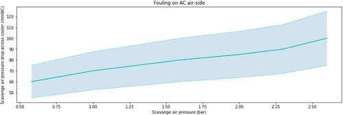
Figure 7 shows a sample of the diagnostic test charts, and in this case of the fouling on the air-side of the AC. The $\mathrm{\Delta }\mathrm{P}\mathrm{C}$ is examined in terms of the $\mathrm{S}\mathrm{C}\mathrm{A}\mathrm{V}\mathrm{\_}\mathrm{A}\mathrm{I}\mathrm{R}\mathrm{\_}\mathrm{P}\mathrm{R}\mathrm{E}\mathrm{S}\mathrm{S}$ and if its value is beyond the highlighted envelope, the test is failed. Failed diagnostic tests occurring when all the cylinders have increased EGT signifies the presence of the respective fault.

Figure 7. Sample diagnostic test for the fouling on the air-side of the AC (This figure is available in colour online.).

3.4.2. Bayesian network and verification

Once the fault mapping is concluded, the results from Table 2 are used to specify the structure of the BN. For the period of interest, the CPTs of the network are populated by aggregating the results from the FD module. After this, virtual and hard evidence regarding the states of the observable and test nodes are used as input. The probabilities of the primary and secondary faults, together with the profile of each fault be obtained using the clustering inference algorithm (Bayes Fusion LLC 2019).

In Figure 8 the resulting layout of the diagnostic BN is shown. The top nodes (i.e. Cyl 1–Cyl 5) represent the state of each cylinder (Failed, Degraded, Normal), based on the residuals’ location in the EWMA control chart for that cylinder. The next layer represents the control nodes, which are tasked with accessing if a simultaneous increase in the ME EGT of all the cylinders takes place. The state of these nodes is binary (True or False). The next two layers represent the primary and secondary fault nodes, each of which has a Normal or Abnormal state. Lastly, the lowest layer represents the test nodes which help to quantify the probability of the occurrence of a specific fault and have Pass or Fail states.

Figure 8. BN structure showing the entire ME system. Observable nodes are located on the top, followed by the control nodes, primary faults, secondary faults and test nodes (This figure is available in colour online.).

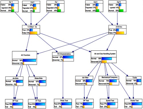
Indicatively, on 23 January 2017, the EWMA control charts suggest that the ME cylinders are on the ‘Failed’ state (hard evidence), as presented in Figure 6. By aggregating the results in the EWMA control charts of each cylinder, between the beginning of the recordings and the 23 January 2017, the following percentages are used as inputs in the CPT of each cylinder (Figure 8):

• Cylinder 1: 36% Failed, 29% Degraded and 36% Normal

• Cylinder 2: 37% Failed, 44% Degraded and 19% Normal

• Cylinder 3: 29% Failed, 22% Degraded and 49% Normal

• Cylinder 4: 34% Failed, 22% Degraded and 44% Normal

• Cylinder 5: 28% Failed, 14% Degraded and 59% Normal

The combination of the CPTs and the ‘Failed’ state in the observable nodes increase the probabilities of the primary and secondary faults. Assuming that the AC pressure-drop test fails, as described in Table 2, Figure 9 is obtained. In this case, the air-side of the AC moves to 100% abnormal state. Also, the level of AC function moves to 86% abnormal state.

Figure 9. BN structure in the presence of fouling in the air-side of the AC (This figure is available in colour online.).

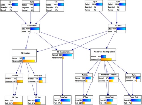
The CPTs of the observable nodes are populated by summarising the amount of data in the different regions of the EWMA control chart of each cylinder. Also, the CPTs of the test and the control nodes are populated to depict functional dependencies in the network. Lastly, the CPTs of the primary and secondary nodes are populated by obtaining failure statistics from Offshore and Onshore Reliability Data (OREDA) data-bank and using logical rules, due to the absence of available parameters from the used data acquisition.

The artificial fault described in Section 3.3.1 is used to assess the ability of the BN in finding the root cause of developing faults. Increased residuals are obtained for each cylinder and the results of the EWMA charts are summarised to populate the corresponding nodes. Subsequently, gradual transitions between each state of the observable nodes, through the use of virtual evidence, takes place. The transition concludes at the Fail state in all the observable nodes, which is facilitated using hard evidence. This process is repeated and applied similarly for each of the test nodes.

Hard evidence is used to demonstrate the BNs ability to calculate the probability of observing each fault. Therefore, the observable nodes are set at the Fail state, due to the artificial fault, and the appropriate test nodes are set to the Fail state. The application of the virtual evidence follows the same principle, but their use allows to capture the profile of each fault (i.e. the cause for the artificial fault). Figures 10 and 11 show the fault profiles for the primary and secondary faults respectively, as verified by the data provider. Regarding the primary faults shown in Figure 10, the possible failure modes are examined and summarised in Table 3.

Figure 10. Fault profiles for the primary faults including all the failure modes (This figure is available in colour online.).

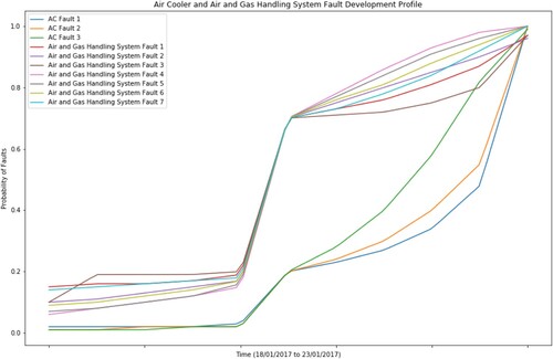
Figure 11. Fault profiles for the secondary faults (This figure is available in colour online.).

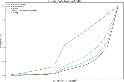
Table 3. Failure modes summary for the primary faults.

Case Number	Failure Modes
AC Fault 1	AC Water-side fouling
AC Fault 2	AC Air-side fouling
AC Fault 3	AC Air-side fouling AC Water-side fouling
Air and Gas Handling System Fault 1	AF Fouling
Air and Gas Handling System Fault 2	Corroded TC mechanical components
Air and Gas Handling System Fault 3	TC fouling
Air and Gas Handling System Fault 4	AF Fouling Corroded TC mechanical components TC fouling
Air and Gas Handling System Fault 5	AF Fouling Corroded TC mechanical components
Air and Gas Handling System Fault 6	Corroded TC mechanical components TC fouling
Air and Gas Handling System Fault 7	AF Fouling TC fouling

Figure 10 shows the fault profiles for the primary faults based on Table 3. In Figure 10, the lower three lines represent the failure modes of the AC, whereas the remaining represent the failure modes of the air and gas handling system. As observed, the air and gas handling system have a faster fault development profile than the AC. Consequently, simultaneous deviations in the ME EGT are more likely to be caused by faults in the air and gas handling system. In particular, the fastest developing failure mode corresponds to the simultaneous failure of all the components of the air and gas handling system.

Figure 11 shows the fault profiles for the secondary faults, observing that the fastest developing fault profile belongs to the corroded TC mechanical components followed by the AF fouling. Therefore, corrosion in the mechanical components of the TC is the fault that can develop the fastest in the system. Therefore, during the period of interest any faults manifested through the simultaneous increase of the ME EGT, are most likely attributed to the corrosion of the mechanical components of the TC.

4. Conclusions

The focus of this paper is the development of a novel diagnostic framework for practical applications in ship systems combining BNs and machine learning. In detail, the novelty of this paper lies in the combination of ML-based FD with BNs for practical ship system diagnostics. Also, another novel part is the use of both hard and virtual evidence for capturing the profiles of different faults. The aim is to improve ship safety and obtain an enhanced understanding of the operational condition for marine engineering systems in a practical manner. For this, DBCSAN and data filtering are used for pre-processing, multiple PRR and EWMA are used for FD, while fault mapping and a BN are used for the diagnostic task and for obtaining the fault profiles of the different faults and failure modes. In detail, the key outcomes of this study are the following:

• The development of a novel diagnostic framework for practical applications in ship systems, enriching the lacking literature.

• The creation of a practical diagnostic network allows the real-time assessment of operational data to compute accurate probabilities of different faults.

• The use of the fault probabilities to better understand the operation state of the examined system and to improve ship safety.

• The novel integration of machine learning applications for pre-processing and FD with BNs for diagnostic tasks.

• The development of robust machine learning based FD and pre-processing modules.

• The integration of domain knowledge with data from data-banks and results from the machine learning based FD for the population of the CPTs of the BN.

• The ability to obtain the fault profiles for different faults and failure modes, which allows the comparison of different failure modes, based on the rate with which they develop.

Future work can include the expansion of the BN for the modelling of other systems (e.g. diesel generator system), keeping in mind that only variables whose behaviour can be predicted through EB modelling can be used. Additionally, another limitation is the use of data banks in the absence of available data from the data acquisition system. From the point of view of practicality, the developed framework can be used to monitor the degradation of systems over time while capturing trends caused by the ship’s operating profile. Additionally, the real-time detection of developing faults and the identification of the root cause can help operators evaluate the condition of vessels and better plan and manage the required maintenance. Consequently, FD and diagnostics can trickle down and improve the operational efficiency, and ultimately the profitability of vessels.

Acknowledgement

This publication reflects only the authors' views and Innovate UK is not liable for any use that may be made of the information contained within.

Disclosure statement

No potential conflict of interest was reported by the author(s).

Additional information

Funding

The work presented in this paper is partially funded by the Integrated Ship Energy and Maintenance Management System (ISEMMS) Project No TP102435 under the Technology Programme Managing Energy on Marine Vessels Competition for Funding.

References

- Adegoke NA, Abbasi SA, Dawod ABA, Pawley MDM. 2019. Enhancing the performance of the EWMA control chart for monitoring the process mean using auxiliary information. Qual Reliab Eng Int [Internet]. [accessed 2019 Jul 13]. 35(4):920–933. https://onlinelibrary.wiley.com/doi/abs/10.1002/qre.2436.
- Amin T, Khan F, Imtiaz S. 2018, October. Fault detection and pathway analysis using a dynamic Bayesian network. Chem Eng Sci [Internet]. DOI:10.1016/j.ces.2018.10.024.
- Atoui MA, Verron S, Kobi A. 2015. Fault detection and diagnosis in a Bayesian network classifier incorporating probabilistic boundary. IFAC-PapersOnLine. 28(place unknown):670–675.
- Babaleye A, Kurt R. 2020. Safety analysis of offshore decommissioning operation through Bayesian network. Ships Offshore Struct. 15(1):99–109.
- Badodkar DN, Dwarakanath TA. 2017. Machines, mechanism and robotics. In: Badodkar DN, Dwarakanath TA, editors. Proceeding INA 2017 [Internet]. 1st ed. Mumbai: Springer; p. 841; http://link.springer.com/10.1007/978-981-10-8597-0.
- Bangalore P, Patriksson M. 2018. Analysis of SCADA data for early fault detection, with application to the maintenance management of wind turbines. Renew Energy [Internet]. [accessed 2019 Jan 25]. 115:521–532. https://linkinghub.elsevier.com/retrieve/pii/S0960148117308340.
- Bayes Fusion LLC. 2019. GeNIe Modeler. Genie.:588.
- Bilmes J. 2004. On virtual evidence and soft evidence in Bayesian networks. Seattle. http://www.ee.washington.edu.
- Bowerman BL, O’Connell RT, Murphree ES. 2015. Regression analysis unified concepts, practical applications, and computer implementation. [place unknown].
- Cai B, Huang L, Xie M. 2017. Bayesian networks in fault diagnosis. IEEE Trans Ind Informatics. 13(5):2227–2240.
- Cai B, Liu H, Xie M. 2016. A real-time fault diagnosis methodology of complex systems using object-oriented Bayesian networks. Mech Syst Signal Process. 80:31–44.
- Campora U, Cravero C, Zaccone R. 2018. Marine gas turbine monitoring and diagnostics by simulation and pattern recognition. Int J Nav Archit Ocean Eng [Internet]. 10(5):617–628. DOI:10.1016/j.ijnaoe.2017.09.012.
- Çelik M, Dadaşer-Çelik F, Dokuz AŞ. 2011. Anomaly detection in temperature data using DBSCAN algorithm. INISTA 2011 – 2011 International Symposium on Innovations in Intelligent Systems and Applications. p. 91–95.
- Cheliotis M, Gkerekos C, Lazakis I, Theotokatos G. 2019. A novel data condition and performance hybrid imputation method for energy efficient operations of marine systems. Ocean Eng. 188. DOI:10.1016/j.oceaneng.2019.106220.
- Cheliotis M, Lazakis I, Theotokatos G. 2020. Machine learning and data-driven fault detection for ship systems operations. Ocean Eng [Internet]. 216(September):107968. https://linkinghub.elsevier.com/retrieve/pii/S0029801820309203.
- Chen Z, Li YF. 2011. Anomaly detection based on enhanced DBScan algorithm. Procedia Eng [Internet]. [accessed 2019 Jun 26]. 15:178–182. https://www.sciencedirect.com/science/article/pii/S1877705811015372.
- Chojnacki E, Plumecocq W, Audouin L. 2019. An expert system based on a Bayesian network for fire safety analysis in nuclear area. Fire Saf J [Internet]. 105(October 2018):28–40. DOI:10.1016/j.firesaf.2019.02.007.
- Coraddu A, Oneto L, Cipollini F, Kalikatzarakis M. 2021. Physical, data-driven and hybrid approaches to model engine exhaust gas temperatures in operational conditions. Ships Offshore Struct. 1–22. DOI:10.1080/17445302.2021.1920095.
- Diakaki C, Panagiotidou N, Pouliezos A, Kontes GD, Stavrakakis GS, Belibassakis K, Gerostathis TP, Livanos G, Pagonis DN, Theotokatos G. 2015. A decision support system for the development of voyage and maintenance plans for ships. Int J Decis Support Syst. 1:42–71.
- Dikis K, Lazakis I, Theotokatos G. 2015. Dynamic reliability analysis tool for ship machinery maintenance. Towar Green Mar Technol Transp. 619–626.
- EMSA. 2018. Annual overview of marine casualties and incidents 2018 [Internet]. Lisbon. http://www.emsa.europa.eu/publications/technical-reports-studies-and-plans/download/5425/3406/23.html.
- Gaonkar M, Sawant K. 2013. Auto Eps DBSCAN: DBSCAN with Eps automatic for large dataset. Int J Adv Comput Theory Eng. 2(2):11–16.
- Garoudja E, Harrou F, Sun Y, Kara K, Chouder A, Silvestre S. 2017. Statistical fault detection in photovoltaic systems. Sol Energy [Internet]. 150:485–499. DOI:10.1016/j.solener.2017.04.043.
- Harrou F, Nounou MN, Nounou HN, Madakyaru M. 2015. PLS-based EWMA fault detection strategy for process monitoring. J Loss Prev Process Ind [Internet]. [accessed 2019 Feb 7]. 36:108–119. DOI:10.1016/j.jlp.2015.05.017.
- Homik W. 2010. Diagnostics, maintenance and regeneration of torsional vibration dampers for crankshafts of ship diesel engines. Polish Marit Res. 17(1):62–68.
- Horný M. 2014. Bayesian networks: A technical report. Commun ACM [Internet]. 53(5):15. http://www.bu.edu/sph/files/2014/05/bayesian-networks-final.pdf%0Ahttp://portal.acm.org/citation.cfm?doid=1859204.1859227.
- Hountalas DT. 2000. Prediction of marine diesel engine performance under fault conditions. Appl Therm Eng. 20(18):1753–1783.
- Isermann R. 2006. Fault-diagnosis systems. In: Isermann R, editor. An introduction from fault detection to fault tolerance [Internet]. Darmstadt: Springer; [accessed 2019 Jun 24]. https://link.springer.com/content/pdf/10.1007%2F3-540-30368-5.pdf.
- ISO. 2008. ISO 3046-1:2002 Reciprocating internal combustion engines: performance: Part 1: declarations of power, fuel and lubricating oil consumptions, and test methods: additional requirements for engines for general use [Internet]; p. 40. https://www.iso.org/standard/28330.html.
- Jardine AKS, Lin D, Banjevic D. 2006. A review on machinery diagnostics and prognostics implementing condition-based maintenance. Mech Syst Signal Process. 20(7):1483–1510.
- Karatug C, Arslanoglu Y. 2020. Importance of early fault diagnosis for marine diesel engines: a case study on efficiency management and environment. Ships Offshore Struct. 15:1–9.
- Karvelis P, Georgoulas G, Kappatos V, Stylios C. 2021. Deep machine learning for structural health monitoring on ship hulls using acoustic emission method. Ships Offshore Struct. 16(4):440–448.
- Kobbacy KA. 2008. Complex system maintenance handbook. 1st ed. New Jersey: Springer.
- Korb KB, Nicholson AE. 2010. Bayesian artificial intelligence. 2nd ed. New York: CRC Press.
- Korczewski Z. 2016. Exhaust gas temperature measurements in diagnostics of turbocharged marine internal combustion engines Part II dynamic measurements. Polish Marit Res. 23(1):68–76.
- Kotsiantis SB, Kanellopoulos D, Pintelas PE. 2006. Data preprocessing for supervised learning. Int J Comput Sci [Internet]. 1(2):111–117. http://citeseerx.ist.psu.edu/viewdoc/download?doi=10.1.1.132.5127&rep=rep1&type=pdf.
- Langseth H, Portinale L. 2007. Bayesian networks in reliability. Reliab Eng Syst Saf. 92(1):92–108.
- Law AM. 2009. How to build valid and credible simulation models. Proceedings – Winter Simulation Conference; p. 24–33.
- Lazakis I, Gkerekos C, Theotokatos G. 2018. Investigating an SVM-driven, one-class approach to estimating ship systems condition. Ships Offshore Struct. 14:432–441.
- Lazakis I, Turan O, Aksu S. 2010. Increasing ship operational reliability through the implementation of a holistic maintenance management strategy. Ships Offshore Struct [Internet]. [accessed 2020 Jan 22]. 5(4):337–357. http://www.tandfonline.com/doi/abs/10.1080/17445302.2010.480899.
- MAN B&W. 2014. Influence of ambient temperature conditions. Copenhagen: MAN Diesel and Turbo.
- MAN B&W. 2017. Operational and maintenance manual. Operating Manuals. 1(1):1438.
- Martinez-Guerra R, Luis Mata-Machuca J. 2013. In: Martinez-Guerra R, Luis Mata-Machuca J, editors. Understanding complex systems fault detection and diagnosis in nonlinear systems: A differential and algebraic viewpoint [Internet]. London: Springer; [accessed 2019 Jun 24]. http://www.springer.com/series/5394.
- McKee KK, Forbes GL, Mazhar I, Entwistle R, Howard I. 2014. Engineering Asset Management 2011: Proceedings of the Sixth World Congress on Engineering Asset Management. In: Lee J, Ni J, Sarangapani J, Mathew J, editors. 1st ed. London: Springer; p. 259–272.
- Mohanty AR. 2015. Machinery condtion monitoring. 1st ed. [place unknown]: Taylor & Francis.
- Mrad AB, Delcroix V, Maalej MA, Piechowiak S, Abid M. 2012. Communications in Computer and information science. In: Greco S, Bouchon-Meunier B, Coletti G, Fedrizzi M, Matarazzo B, Yager R, editors. Advances in Computational intelligence. Catania: Springer; p. 626.
- Müller AC, Guido S. 2015. Introduction to Machine Learning with Python and Scikit-Learn. 1st ed. Schanafelt D, editor. Sebastopol: O’Reily. http://kukuruku.co/hub/python/introduction-to-machine-learning-with-python-andscikit-learn.
- Nounou M, Nounou H, Mansouri M, Harkat MF, Al-khazraji A, Hajji M. 2018. Wavelet optimized EWMA for fault detection and application to photovoltaic systems. Sol Energy [Internet]. [accessed 2019 Feb 7]. 167:125–136. https://linkinghub.elsevier.com/retrieve/pii/S0038092X18303050.
- Olive DJ. 2005. Linear regression. 1st ed. Cham: Springer.
- Rahmah N, Sitanggang IS. 2016. Determination of Optimal Epsilon (Eps) value on DBSCAN Algorithm to Clustering Data on Peatland Hotspots in Sumatra. In: IOP Conference Series: Earth Environmental Science. Vol. 31. [place unknown]; p. 12012.
- Ranachowski Z, Bejger A. 2005. Fault diagnostics of the fuel injection system of a medium power maritime diesel engine with application of acoustic signal. Arch Acoust. 30(4):465–472.
- Raptodimos Y, Lazakis I. 2018. Using artificial neural network-self-organising map for data clustering of marine engine condition monitoring applications. Ships Offshore Struct [Internet]. 13(6):649–656. DOI:10.1080/17445302.2018.1443694.
- Riascos LAM, Simoes MG, Miyagi PE. 2007. A Bayesian network fault diagnostic system for proton exchange membrane fuel cells. J Power Sources [Internet]. [accessed 2019 Mar 5]. 165(1):267–278. https://www.sciencedirect.com/science/article/pii/S0378775306025262.
- Ruggeri F, Faltin F, Kenett R. 2007. Bayesian networks. Wiley Interdiscip Rev Comput Stat [Internet]. 1(3):307–315. DOI:10.1002/wics.48.
- Saltelli A. 2004. Sensitivity analysis in practice: a guide to assessing scientific models (Google eBook) [Internet]. [place unknown]. http://books.google.com/books?id=NsAVmohPNpQC&pgis=1.
- Schlechtingen M, Santos IF. 2014. Wind turbine condition monitoring based on SCADA data using normal behavior models. part 2: application examples. Appl Soft Comput J [Internet]. [accessed 2019 Jan 25]. 14(PART C):447–460. DOI:10.1016/j.asoc.2013.09.016.
- Schlechtingen M, Santos IF, Achiche S. 2013. Wind turbine condition monitoring based on SCADA data using normal behavior models. Part 1: system description. Appl Soft Comput J [Internet]. [accessed 2019 Jan 24]. 13(1):259–270. DOI:10.1016/j.asoc.2012.08.033.
- Schubert E, Sander J, Ester M, Kriegel HP, Xu X. 2017. DBSCAN revisited, revisited: Why and how you should (still) use DBSCAN. ACM Trans Database Syst. 42(3):1–21.
- Silva AA, Gupta S, Bazzi AM, Ulatowski A. 2018. Wavelet-based information filtering for fault diagnosis of electric drive systems in electric ships. ISA Trans [Internet]. [accessed 2019 Sep 23]. 78:105–115. https://linkinghub.elsevier.com/retrieve/pii/S001905781730544X.
- Tan Y, Niu C, Tian H, Lin Y, Zhang J. 2020. Decay detection of a marine gas turbine with contaminated data based on isolation forest approach. Ships Offshore Struct. 16(5):546–556.
- Tanasa D, Trousse B. 2004. Advanced data preprocessing for intersites Web usage mining. Intell Syst IEEE. 19(2):59–65.
- Tantele EA, Onoufriou T. 2009. Optimum preventative maintenance strategies using genetic algorithms and Bayesian updating. Ships Offshore Struct [Internet]. 5302. http://www.tandfonline.com/doi/abs/10.1080/17445300903247162.
- Thang TM, Kim J. 2011. The anomaly detection by using DBSCAN clustering with multiple parameters. 2011 Int Conf Inf Sci Appl ICISA 2011.:1–5.
- Theotokatos G, Tzelepis V. 2015. A computational study on the performance and emission parameters mapping of a ship propulsion system. Proc Inst Mech Eng Part M J Eng Marit Environ. 229(1):58–76.
- Turan O, Olcer AI, Lazakis I, Rigo P, Caprace JD. 2009. Maintenance/repair and production-oriented life cycle cost/earning model for ship structural optimisation during conceptual design stage. Ships Offshore Struct. 4(2):107–125.
- Wang J, Wang Z, Stetsyuk V, Ma X, Gu F, Li W. 2019. Exploiting Bayesian networks for fault isolation: a diagnostic case study of diesel fuel injection system. ISA Trans [Internet]. 86:276–286. DOI:10.1016/j.isatra.2018.10.044.
- Wang Z, Zhiwei W, He S, Gu X, Yan ZF. 2017. Fault detection and diagnosis of chillers using Bayesian network merged distance rejection and multi-source non-sensor information. Appl Energy. 188:200–214.
- Woodyard D. 2009. In: Butterworth Heineman, editor. Manire diesel engines and gas turbines. 9th ed. Oxford: Elsevier.
- Yu J, Smith VA, Wang PP, Hartemink AJ, Jarvis ED. 2004. Advances to Bayesian network inference for generating causal networks from observational biological data. Bioinformatics. 20(18):3594–3603.
- Zaher A, McArthur SDJ, Infield DG, Patel Y. 2009. Online wind turbine fault detection through automated SCADA data analysis. Wind Energy. 12(6):574–593.
- Zhan Y, Bin SZ, Shwe T, Wang XZ. 2007. Fault diagnosis of marine main engine cylinder cover based on vibration signal. In: Proceedings of the Sixth International Conference Machine Learning and Cybernetics ICMLC 2007 [Internet]. Vol. 2. [place unknown]: IEEE; [accessed 2019 Jun 25]; p. 1126–1130. http://ieeexplore.ieee.org/document/4370313/.
- Zhao Y, Wen J, Xiao F, Yang X, Wang S. 2017. Diagnostic Bayesian networks for diagnosing air handling units faults – part I: faults in dampers, fans, filters and sensors. Appl Therm Eng. 111:1272–1286.
- Zheng X, Yao W, Xu Y, Chen X. 2019. Improved compression inference algorithm for reliability analysis of complex multistate satellite system based on multilevel Bayesian network. Reliab Eng Syst Saf [Internet]. 189(March):123–142. DOI:10.1016/j.ress.2019.04.011.