Dynamic motion response of an oil tanker moored with a single buoy under different mooring system failure scenarios

ABSTRACT

In this study, the dynamic responses of an oil tanker moored on a Catenary Anchor Leg Mooring (CALM) buoy were simulated under the wave, wind and current through numerical simulations. Then the tension of the mooring lines and the drift range of the tanker were studied after a mooring system failure. Simulations were done with ANSYS AQWA and Orcina OrcaFlex. Hydrodynamics of tanker was first solved in the frequency domain through AQWA based on the potential theory, three-dimensional radiation and diffraction theory. Then coupled dynamic models, including buoy, oil tanker and the mooring system, were calculated using OrcaFlex. Two mooring system failure scenarios, including the continuous failure of two anchor chains and the failure of hawser, were simulated. The drift ranges of the tanker, hawser and anchor chain tension after the mooring system failure were discussed. The obtained results from this study can be provided as a reasonable reference for ports and related departments for emergency responses.

KEYWORDS:

• Oil tanker
• Catenary Anchor Leg Mooring buoy
• mooring system failure
• anchor chain
• hawser
• drift range

1. Introduction

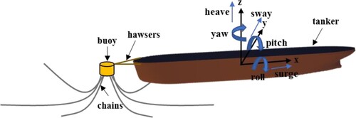
Due to insufficient water depth in the port, larger oil tankers cannot approach ports for offloading and loading. Therefore, there are many different terminals located offshore, outside port or in sheltered anchorage areas. Since the 1960s, single point mooring (SPM) systems have become popular for offshore loading or offloading gas or liquid products. The Catenary Anchor Leg Mooring (CALM) system is one of the forms. The basic principle of the buoy is to keep the tanker's position stable relative to the buoy, while allowing the tanker to swing with the wind, wave and current. The components of the system are the body of the buoy, mooring and anchoring elements, product transfer system and ancillary components. The buoy is fixed by positioning it in the centre of four to eight anchor chains connected to it. The tanker is moored to the buoy with one or two hawsers. Rutkowski (2019) described the characteristics of SPM and hydro-meteorological condition limits enabling safe ship’s cargo and manoeuvring operation offshore. Product offloading is possible with the wind up to 40 knots and head waves of 3.0–4.5 m.

Wichers (1976) studied the general SPM mooring problem of the slowly varying drifting behaviour of the object moored through a bow hawser. Bernitsas and Papoulias (1986) used a mathematical model for the horizontal plane slow motions of ships connected to an SPM. The influences of the wind, waves and current on the dynamic of single-point moored vessels were investigated (Sharma et al. 1994; Schellin 2007; Wang et al. 2007). Esmailzadeh and Goodarzi (2001) used a mathematical model to show that the governing equation of motion for the system is a non-linear parametric second-order ordinary differential equation. Sagrilo et al. (2002) presented a time-domain finite element-based numerical procedure to perform a coupled dynamic analysis of the system consisting of a buoy and its slender structures under environmental random loads. Schellin (2003) analysed the comparative simulated time histories of the mooring load and the corresponding horizontal motion response for the SPM tankers. Chang et al. (2012) modelled an SPM buoy system by applying the multi-body dynamics method. Kang et al. (2014) analysed the response of FPSO and CALM offloading systems under special environmental conditions in West Africa. Several studies improved the performance of SPM (Paulauskas 2009; Eghbali et al. 2018). Lee and Kim (2019) performed an SPM mooring safety assessment using OPTIMOOR to understand the mooring characteristics of SPM.

Recently, Amaechi et al. (2021a, 2021b, 2021a) presented a review of theoretical, numerical, and experimental investigations on hoses and an overview of different systems applied in sustainable fluid transfer and (un)loading operations by these marine structures. Numerical simulation and experiment of submarine hose systems attached to CALM buoys have been studied (Amaechi et al. 2019; Amaechi et al. 2021b, 2022a). The hydrodynamic analysis of the disconnection-induced load response of marine-bonded hoses attached to a CALM buoy and the CALM buoy motion response, the effect of buoy skits and the effect of buoy geometries were investigated through numerical simulation (Amaechi et al. 2022c, 2022d). Amaechi et al. (2022b) showed hydrodynamic characteristics of CALM buoy hose systems under the wind, waves and current.

Some of the studies discussed mooring system failure by bending. The consequences of mooring failure will have an environmental impact and business interruption impact. Brown et al. (2005) discussed the causes of system degradation and the consequences of mooring failure to investigate how to improve the integrity of the moorings by floating production systems. There is a possibility of failure of continuous mooring lines. In 2004, a December North Sea storm resulted in a drilling rig losing two of its eight anchor chains. The resulting excessive excursions ruptured the drilling riser.

In this study, the dynamic responses of an oil tanker that was moored on a CALM buoy were simulated under the wave, wind and current through a time-domain numerical model. Then the tension of the mooring lines and the drift range of the tanker were studied after a mooring system failure. Hydrodynamics of the tanker was first solved in the frequency domain through AQWA based on the potential theory, three-dimensional radiation and diffraction theory. Then coupled dynamic models, including buoy, oil tanker and the mooring system, were calculated using OrcaFlex.

2. Numerical simulation description

Numerical simulation was calculated by ANSYS AQWA and Orcina OrcaFlex. The target site was selected offshore of 36 m water depth outside Kaohsiung Port, Taiwan. The motion of the oil tanker moored on a single buoy mooring system and the tension of the mooring lines were analysed under operation conditions with the wave, wind, and current forces. In the simulation, the motion of the tanker was computed by many external coupling forces, including external environmental forces, hydrodynamic forces of the tanker, and mooring forces from anchor chains and hawsers. The hydrodynamic model was first established by AQWA to determine the hydrodynamic forces of the tanker in the frequency domain. Then incorporation into the Orcaflex model for coupled dynamic was investigated in the time domain. Figure 1 shows a schematic of the CALM system and the six degrees of freedom of the tanker.

Figure 1. Schematic of the CALM system and the six degrees of freedom of the tanker. (This figure is available in colour online.)

2.1. Tanker model

Dyne Tanker (Ship Viscous Flow Conference, 1990) was the target tanker model (Figure 2). Table 1 shows the properties of the Dyne Tanker under full load conditions.

Figure 2. Dyne Tanker in ANSYS AQWA. (This figure is available in colour online.)

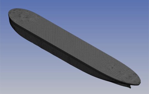
Table 1. Properties of the Dyne Tanker.

Dyne Tanker properties (Full load)
Length overall (m)	263
Length between perpendicular (m)	253
Breadth (m)	38
Depth (m)	19
Draft (m)	14.25
Mass (tonne)	119,311
XCG (m)	118.3
YCG (m)	0
ZCG (m)	−6.65
Moment of Inertia, Ixx (tonne m^2)	21.47 × 10^6
Moment of Inertia, Iyy (tonne m^2)	515.78 × 10^6
Moment of Inertia, Izz (tonne m^2)	515.78 × 10^6
Position in OracFlex	(−18.433, 0, 0)

2.2. Hydrodynamic model

The hydrodynamic model of the Dyne tanker was established using AQWA (ANSYS 2021). The hydrodynamic loads of tankers are calculated employing the three-dimensional radiation/diffraction theory. Under the assumptions of the open boundary water and the potential flow theory, the general equation of motion of the tanker is presented as follows: (1) $\left(M+M_A\left(\omega \right)\right)\ddot{x}+\mathcal{(}D+B\left(\omega \right))\dot{x}+(K+K_H)x=F_{FK}+F_D$(1) where $M$ is the tanker mass; $M_A$ is the added mass (frequency-dependent); $D$ is the decay coefficient; $B$ is the damping (frequency-dependent); $K$ is the hydrostatic stiffness; $K_H$ is the decay coefficient; $F_{FK}$ is the Froude-Krylov force; $F_D$is the diffracting force and $\ddot{x}$, $\dot{x}$, $x$ are accelerations, velocity, and displacement of the tanker.

Dyne Tanker parameters for calculation were set in the frequency domain. The parameters were 36 m water depth and 1025 kg/m³ seawater density. The wave direction range was −180°∼180°, and the interval was 45°. The maximum element size of mesh was set to 2 m, and the defeaturing tolerance was 0.1 m. The total elements of mesh were 22,525.

2.3. Dynamic model

Coupled dynamic models in the time domain, including buoy, oil tanker and the mooring system, were calculated using OrcaFlex (Orcina 2021). The motion from OrcaFlex is (2) $M\left(p,a\right)+C\left(p,v\right)+K\left(p\right)=F\left(p,v,t\right)$(2) where $M\left(p,a\right)$ is the system inertia load; $C\left(p,v\right)$ is the system damping load; $K\left(p\right)$ is the system stiffness load; $F\left(p,v,t\right)$ is the external load; $p,v,t$ is the position, velocity and acceleration vectors, respectively and $t$ is the simulation time.

The implicit time-domain dynamic integration scheme (Chung and Hulbert 1993) was used. Then the system equation of motion was solved by the time step of 0.03 s.

For hydrodynamic loads on mooring lines and buoys, an extended form of Morison's equation (Morison et al. 1950) was used to calculate the wave loads on the moving body. The extended form of Morison's equation used in OrcaFlex (Orcina 2021) is (3) $f=\left(C_m\mathrm{\Delta }{a}_f+C_a\mathrm{\Delta }{a}_b\right)+{\displaystyle \frac{1}{2}\rho C_{d}A\left|v_r\right|v_r}$(3) where $f$ is the fluid force (per unit length) on the body; $C_m$ is the inertia coefficient for the body; $\mathrm{\Delta }$ is the mass of fluid displaced by the body; $a_f$ is the fluid acceleration relative to the earth; $C_a$ is the added mass coefficient for the body; $a_b$ is the body acceleration relative to the earth; $\rho$ is the density of the water; $C_d$ is the drag coefficient for the body; $A$ is the cross-sectional area of the body and $v_r$ is the fluid velocity relative to the body.

The value of $C_m$ used in OrcaFlex was $1+C_a$. The value of $C_a$ was set to 1.0, and the value of $C_d$ was set to 2.6.

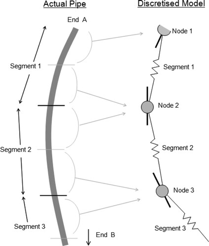
OrcaFlex uses a finite element model for a line shown in Figure 3. The line is divided into a series of line segments, modelled by straight massless model segments with a node at each end. The model segments only model the axial and torsional properties of the line. The other properties (mass, weight, buoyancy) are all lumped into the nodes.

Figure 3. OrcaFlex line model (Orcina 2021). (This figure is available in colour online.)

2.3.1 Buoy body

The buoy (Figure 4) is simplified into a cylinder with a diameter of 12.5 m and a height of 5.8 m. In addition, a turntable was designed on the upper part of the buoy allowing the tanker to swing. Table 2 shows the buoy parameters used in a dynamic model.

Figure 4. Form of buoy body in OrcaFlex. (This figure is available in colour online.)

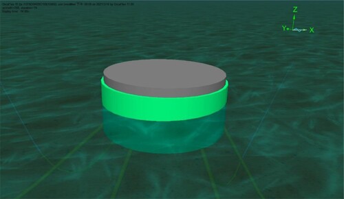
Table 2. Parameters of the buoy.

Buoy’s parameters
Size (ø$\times$H) (m)	12.5 × 5.8
Draft (m)	2.263
Mass (kg)	284,000
XCG (m)	0
YCG (m)	0
ZCG (m)	0.637
Moment of Inertia, Ixx (kg m^2)	3,570,000
Moment of Inertia, Iyy (kg m^2)	3,570,000
Moment of Inertia, Izz (kg m^2)	5,560,000
Position in OrcaFlex	(−173, 0, 0)

2.3.2 Mooring system

As shown in Figure 5, the tanker is moored to the buoy by two hawsers (L1, L2), and the buoy is anchored to the seabed by six catenary anchor chains (M1∼M6). Two hawsers were modelled with 0.246 m polypropylene (8-strand Multiplait) and had a length of 40 m. The anchor chain's nominal diameter was 11.4 cm. A Grade R3 stud-link chain was chosen as the mooring component. The interval angle of each anchor chain was 60°. The unstretched length of the anchor chain was 220 m. Tables 3 and 4 give the properties of hawser and anchor chain, respectively.

Figure 5. CALM system and tanker in OrcaFlex. (This figure is available in colour online.)

Table 3. Properties of the hawser.

Hawser properties
Polypropylene (8-strand Multiplait)
Length (m)	40
Diameter (m)	0.246
Mass per unit length (kg/m)	27.39
Axial stiffness (kN)	64,150
Minimum breaking strength (kN)	6415

Table 4. Parameters of the anchor chain.

Mooring chain properties
Grade R3 stud-link
Number of mooring lines	6*1
Anchor between lines (°)	60
Water depth (m)	36
Radius to anchor from the buoy centreline (m)	215
Length (m)	220
Nominal diameter (m)	0.11
Mass per unit length (kg/m)	286.11
Axial stiffness (kN)	1320,000
Minimum breaking strength (kN)	8925.37

2.4. Simulation of the mooring system failure

The mooring line failure was investigated from the fair lead under the wave, wind and current loads. The mooring system failure scenarios were divided into the continuous failure of M1 & M2 and the failure of L1. As shown in Table 5, the red line represents the failed mooring line. In the scenario I, the failure of anchor chain M1 was set to occur at a simulation time of 5,000th second, and then the failure of anchor chain M2 was set to occur at a simulation time of 6000th second. In the scenario II, the failure of hawser L1 was set to occur at a simulation time of 5000th second.

Table 5. Two mooring system failure scenarios.

Number	Mooring line failure	Schematic
Scenario I	M1 & M2
Scenario II	L1

The drift range of the tanker and the tension of hawsers and anchor chains after the mooring system failure were discussed. The water area of anchorage was adopted in the technical specifications of Chinese Ports and the mooring system tension specification of API RP 2SK (American Petroleum Institute 2005).

In the Chinese Port technical specification, the water area of each anchorage is circular, and its radius $R$ is (4) $R=L+r+l+e$(4) where $L$ is the length overall; $r$ is the horizontal deviation of the buoy caused by the tidal range; $l$ is the horizontal length of the hawser and $e$ is the distance between the stern and the berth boundary, generally 0.1 $L$.

The API RP 2SK specification indicates that the maximum tension limit cannot exceed 60% minimum breaking strength (MBS) of the mooring line in an intact state under dynamic analysis. Moreover, the maximum tension limit cannot exceed 80% MBS of the mooring line in a damaged state under dynamic analysis. Table 6 shows mooring lines 60% MBS and 80% MBS, respectively.

Table 6. Mooring lines’ 60% and 80% minimum breaking strength.

Mooring line	60% MBS (kN)	80% MBS (kN)
Anchor chain	5,355	7140
Hawser	3,849	5132

The environmental conditions used in numerical simulation included irregular waves, uniform current and uniform wind. The irregular wave was simulated by the JONSWAP (Joint North Sea Wave Project) spectrum with a significant wave height $H_s$ of 3 m, significant wave period $T_s$ of 9 s and peak enhancement factor ($\gamma$) of 1.1. The uniform current velocity was 1 m/s and the uniform wind velocity was 20 m/s. The different wind directions and current directions conditions are shown in Tables 7 and 8 and Figure 6.

Figure 6. Directions of environmental conditions. (This figure is available in colour online.)

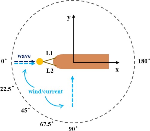
Table 7. Wave and current at the same direction conditions.

Wave conditions			Wind conditions		Current conditions
Hs (m)	Ts (s)	Wave direction (°)	Wind velocity (m/s)	Wind direction (°)	Current velocity (m/s)	Current direction (°)
3	9	0	20	0	1	0
				22.5
				45
				67.5
				90

Table 8. Wave and wind in the same direction conditions.

Wave conditions			Wind conditions		Current conditions
Hs (m)	Ts (s)	Wave direction (°)	Wind velocity (m/s)	Wind direction (°)	Current velocity (m/s)	Current direction (°)
3	9	0	20	0	1	0
						22.5
						45
						67.5
						90

3. Results and discussion

3.1. Numerical model verification in free decay

Based on the Froude number, a 1/100 scale Dyne Tanker experimental model (Figure 7) was used for the free decay test and compared with the numerical simulation. Figure 8 shows time series in heave (a), roll (b) and pitch (c) motions from the simulation and the experiment. Table 9 compares the natural periods of the tanker between the simulation and the experiment. In the experimental test, the natural periods of heave, roll and pitch were 6.48, 7.24 and 7.54 s, respectively. Regarding numerical test, the natural periods of heave and roll were 7.2, 9.05 s and 7.8, respectively. The numerical results showed that the natural simulation periods were slightly bigger than those of the experiment. The deviation can be the centre of gravity and moment of inertia being slightly different from the homogeneity assumption in simulation.

Figure 7. 1/100 scaled Dyne Tanker model. (This figure is available in colour online.)

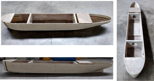
Figure 8. Time series in heave (a), roll (b) and pitch (c) motions of the simulation and the experiment. (This figure is available in colour online.)

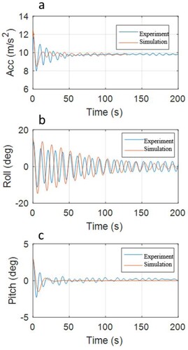
Table 9. Comparison of the natural periods of the tanker between the simulation and the experiment.

Natural period	Heave	Roll	Pitch
Experiment	6.82 s	8.42 s	7.54 s
Simulation	7.2 s	9.05 s	7.8 s

3.2 The continuous failure of anchor chains M1 & M2 (scenario I)

Considering the scenario I, the failure of anchor chain M1 was set to occur at a simulation time of 5000th second, and then the failure of anchor chain M2 was set to occur at a simulation time of 6000th second. The simulation results were divided into stage 1 before the failure of M2 and stage 2 afterwards.

3.2.1 Tension of anchor chains in the scenario I

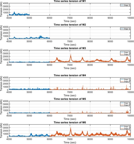
Figure 9 shows time series of anchor chains tension at the wind, wave and current direction of 0°. Figure 10 shows the time series of anchor chains tension at the wave and current direction of 0° and wind direction of 90°. In stage 2, the tension of M3 and M6 gradually increased due to the drift of the buoy. The tension of M4 and M5 did not change obviously when the continuous failure of M1 and M2. However, the continuous failure of M1 and M2 decreased the stability of the buoy, thereby leading the tension of M4 and M5 to increase in a long simulation time considerably.

Figure 9. Time series of anchor chains tension at the wind, wave and current direction of 0° (scenario I). (This figure is available in colour online.)

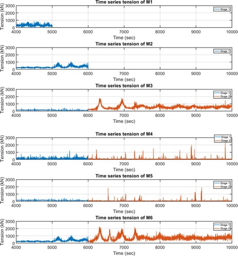
Figure 10. Time series of anchor chains tension at the wave and current direction of 0° and wind direction of 90° (scenario I). (This figure is available in colour online.)

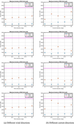
Figure 11 shows the maximum tension of M3, M4, M5 and M6 at different wind/current directions under stage 1 or stage 2. According to the results, the maximum tension of M3, M4, M5 and M6 in stage 2 was larger than in stage 1. In addition, the maximum tension was less than 60% MBS of the anchor chain, representing that even M1 and M2 continuous failures M3, M4, M5 and M6 were still within the safety region.

Figure 11. Maximum tension of M3, M4, M5 and M6 at different wind/current directions under stages 1 and 2 (scenario I). (a) Different wind directions and (b) different current directions. (This figure is available in colour online.)

3.2.2 Tension of hawsers in the scenario I

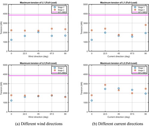
Figure 12 shows the maximum tension of L1 and L2 at different wind/current directions under stage 1 or stage 2. The motion responses of the buoy were increased due to the reduced stability of the anchor chain system, thereby leading the maximum tension of L1 and L2 to increase. In addition, the maximum tension was less than 60% MBS of hawser, representing no immediate damage effect on L1 and L2 in the scenario I.

Figure 12. Maximum tension of L1 and L2 at different wind/current directions under stages 1 and 2 (scenario I). (a) Different wind directions and (b) different current directions. (This figure is available in colour online.)

3.2.3 Drift range of the tanker in the scenario I

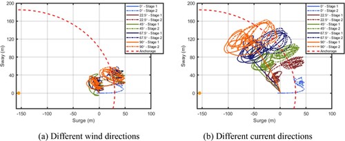
Figure 13 shows the drift range of the tanker at different wind/current directions under stage 1 or stage 2, and the red dashed circle is the water area of anchorage. The drift range of the tanker in different current directions was obviously larger than that in different wind directions because the current force on the tanker was bigger than the wind force. Hence, the influence of the different current directions was more important. In addition, all drift ranges of the tanker exceed the water area of anchorage after the anchor chain M1 and M2 continuous failure, representing that scenario I was not within the specification. It may collide with nearby vessels.

Figure 13. Drift range of the tanker at different wind/current directions under stages 1 and 2 (scenario I). (a) Different wind directions and (b) different current directions. (This figure is available in colour online.)

3.3 The failure of hawser L1 (the scenario II)

In the scenario II, the failure of hawser L1 was about to occur at a simulation time of 5,000th second. The simulation results were divided into stage 1 before the failure of L1 and stage 2 afterwards.

3.3.1 Tension of anchor chains in the scenario II

Figure 14 shows the time series of anchor chains tension at the wind, wave and current direction of 0°. Figure 15 shows the time series of anchor chains tension at the wave and current direction of 0° and wind direction of 90°. In stage 1, the tension of M1 was greater than that of the other anchor chains, because M1 mainly resists the surge motion of the buoy, which has a larger surge dynamic response at a wave direction of 0°. In stage 2, the tension of M1, M2 and M6 considerably increased due to the surge and sway motion responses of the buoy towed by the tanker. The tension of M3, M4 and M5 did not change obviously, which was much smaller than the tension of other anchor chains.

Figure 14. Time series of anchor chains tension at the wind, wave and current direction of 0° (scenario II).

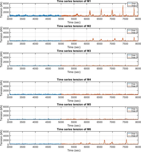
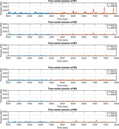
Figure 15. Time series of anchor chains tension at the wave and current direction 0° and wind direction of 90° (scenario II). (This figure is available in colour online.)

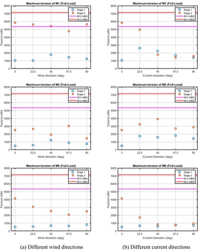
Figure 16 shows the maximum tension of M1, M2 and M6 at different wind/current directions under stage 1 or stage 2. According to the results, the maximum tension of M1, M2 and M6 in stage 2 was larger than in stage 1 except for M1 at the current direction of 45° and 67.5°. In addition, the maximum tension was less than 80% MBS of the anchor chain, representing that the effect of L1 failure on M1, M2 and M6 was still within the specification, but damage risk increased.

Figure 16. Maximum tension of M1, M2 and M6 at different wind/current directions under stages 1 and 2 (scenario II). (a) Different wind directions and (b) different current directions. (This figure is available in colour online.)

3.3.2 Tension of hawsers in the scenario II

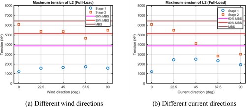
Figure 17 shows the maximum tension of L1 and L2 at different wind/current directions under stage 1 or stage 2. The motion responses on the horizontal plane of the tanker were increased caused by the failure of hawser L1, thereby leading L2 to generate a high tension. In addition, the maximum tension was more than 80% MBS of hawser except for the wind direction of 67.5° and the current direction of 45°, 67.5° and 90°, representing that the effect of L1 failure on L2 was not within the specification, damage risk existed.

Figure 17. Maximum tension of L2 at different wind/current directions under stages 1 and 2 (scenario II). (a) Different wind directions and (b) different current directions. (This figure is available in colour online.)

3.3.3 Drift range of the tanker in the scenario II

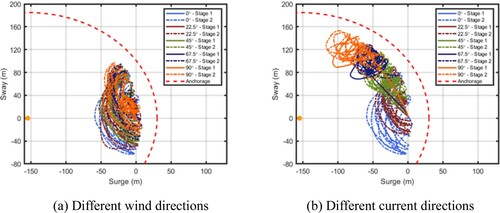
Figure 18 shows the drift range of the tanker at different wind/current directions under stage 1 or stage 2, and the red dashed circle is the water area of anchorage. The drift range of the tanker at different wind directions under stage 2 was larger than that at different current directions. This is because the oscillation on the horizontal plane of the tanker should have happened after the hawser L1 failure. However, the oscillation response of the tanker was smaller due to the limitation of the lateral current force. In addition, all drift ranges of the tanker did not exceed the water area of anchorage after the hawser L1 failure.

Figure 18. Drift range of the tanker at different wind/current directions under stages 1 and 2 (scenario II). (a) Different wind directions (b) Different current directions. (This figure is available in colour online.)

4. Conclusions

The dynamic responses of the oil tanker, which was moored on a CALM buoy, were simulated under the wave, wind and current through a time-domain numerical model. Then the tension of the mooring lines and the drift range of the tanker were studied after a mooring system failure. A simulation was accomplished with ANSYS AQWA and Orcina OrcaFlex. Besides head wave consideration, the environmental conditions selected CALM buoy loading and offloading limit under different wind/current directions. The mooring system failure was divided into two scenarios, including the continuous failure of M1 and M2 (scenario I) and the failure of L1 (scenario II).

The scenario I is simulated for serious accidents, such as continuous mooring line failure. As a result, we can see that the tension of anchor chains and hawsers also did not exceed 60% MBS. However, the drift range of the tanker exceeded the water area of anchorage. It could collide with nearby vessels and cause more serious damage offshore. In addition, the strength of the hawser is much lower than that of the anchor chain, so the scenario II was designed to analyse the failure of the hawser L1. After the failure of L1, it significantly affects the increase in the tension of mooring lines. The maximum tension of hawser L2 exceeded 80% MBS, and there is a risk of damage. Therefore, immediate rescue is needed to take for avoiding subsequent severe disasters.

Disclosure statement

No potential conflict of interest was reported by the author(s).

References

- Amaechi CV, Chesterton C, Butler HO, Wang F, Ye J. 2021a. An overview on bonded marine hoses for sustainable fluid transfer and (un) loading operations via floating offshore structures (FOS). J Mar Sci Eng. 9(11):1236. doi:10.3390/jmse9111236.
- Amaechi CV, Chesterton C, Butler HO, Wang F, Ye J. 2021b. Review on the design and mechanics of bonded marine hoses for Catenary Anchor Leg Mooring (CALM) buoys. Ocean Eng. 242:110062. doi:10.1016/j.oceaneng.2021.110062.
- Amaechi CV, Wang F, Hou X, Ye J. 2019. Strength of submarine hoses in Chinese-lantern configuration from hydrodynamic loads on CALM buoy. Ocean Eng. 171:429–442. doi:10.1016/j.oceaneng.2018.11.010.
- Amaechi CV, Wang F, Ye J. 2021a. Mathematical modelling of bonded marine hoses for single point mooring (SPM) systems, with Catenary Anchor Leg Mooring (CALM) buoy application—a review. J Mar Sci Eng. 9(11):1179. doi:10.3390/jmse9111179.
- Amaechi CV, Wang F, Ye J. 2021b. Numerical assessment on the dynamic behaviour of submarine hoses attached to CALM buoy configured as lazy-S under water waves. J Mar Sci Eng. 9(10):1130. doi:10.3390/jmse9101130.
- Amaechi CV, Wang F, Ye J. 2022a. Experimental study on motion characterisation of CALM buoy hose system under water waves. J Mar Sci Eng. 10(2):204. doi:10.3390/jmse10020204.
- Amaechi CV, Wang F, Ye J. 2022b. Investigation on hydrodynamic characteristics, wave–current interaction and sensitivity analysis of submarine hoses attached to a CALM buoy. J Mar Sci Eng. 10(1):120. doi:10.3390/jmse10010120.
- Amaechi CV, Wang F, Ye J. 2022c. Numerical studies on CALM buoy motion responses and the effect of buoy geometry cum skirt dimensions with its hydrodynamic waves-current interactions. Ocean Eng. 244:110378. doi:10.1016/j.oceaneng.2021.110378.
- Amaechi CV, Wang F, Ye J. 2022d. Understanding the fluid–structure interaction from wave diffraction forces on CALM buoys: numerical and analytical solutions. Ships Offsh Struct. 1–29. doi:10.1080/17445302.2021.2005361.
- American Petroleum Institute. 2005. API RP 2SK: design and analysis of stationkeeping systems for floating structures. https://global.ihs.com/doc_detail.cfm?document_name = API%20RP%202SK&item_s_key = 00226348.
- ANSYS. 2021. AQWA theory manual_R1. ANSYS Inc, Canonsburg, USA. https://pdfcoffee.com/aqwa-theory-manual-2-pdf-free.html.
- Bernitsas MM, Papoulias FA. 1986. Stability of single point mooring systems. Appl Ocean Res. 8(1):49–58. doi:10.1016/S0141-1187(86)80031-1.
- Brown MG, Hall T, Marr D, English M, Snell R. 2005. Floating production mooring integrity JIP-key findings. Paper presented at the offshore technology conference; Houston, Texas, May 2005. doi:.10.4043/17499-MS.
- Chang Z-y, Tang Y-g, Li H-j, Yang J-m, Wang L. 2012. Analysis for the deployment of single-point mooring buoy system based on multi-body dynamics method. China Ocean Eng. 26(3):495–506. doi:10.1007/s13344-012-0037-x.
- Chung J, Hulbert GM. 1993. A time integration algorithm for structural dynamics with improved numerical dissipation: the generalized-α method. J Appl Mech. 60(2): 371–375. doi:10.1115/1.2900803.
- Eghbali B, Daghigh M, Daghigh Y, Azarsina F. 2018. Mooring line reliability analysis of single point mooring (SPM) system under extreme wave and current conditions. Int J Marit Technol. 9:41–49. http://ijmt.ir/browse.php?a_id=631&sid=1&slc_lang=en.
- Esmailzadeh E, Goodarzi A. 2001. Stability analysis of a CALM floating offshore structure. Int J Non-Linear Mech. 36(6):917–926. doi:10.1016/S0020-7462(00)00055-X.
- Kang Y, Sun L, Kang Z, Chai S. 2014. Coupled analysis of FPSO and CALM buoy offloading system in West Africa. Paper presented at the International Conference on offshore Mechanics and Arctic engineering; San Francisco, California, USA. doi:10.1115/OMAE2014-23118.
- Lee S-W, Kim Y-D. 2019. A study on improvement of criteria for mooring safety assessment in single point mooring. J Korean Soc Mar Environ Saf. 25(3):287–297. doi:10.7837/kosomes.2019.25.3.287.
- Morison J, Johnson J, Schaaf S. 1950. The force exerted by surface waves on piles. J Pet Technol. 2(05):149–154. doi:10.2118/950149-G.
- Orcina. 2021. OrcaFlex Manual, Version 11.1b: Ulverton. Orcina Ltd, Cumbria, UK. https://www.orcina.com/webhelp/OrcaFlex/Default.htm.
- Paulauskas V. 2009. The safety of tankers and single point mooring during loading operations. Transport. 24(1):54–57. doi:10.3846/1648-4142.2009.24.54-57.
- Rutkowski G. 2019. A comparison between conventional buoy mooring CBM, single point mooring SPM and single anchor loading SAL systems considering the hydro-meteorological condition limits for safe ship’s operation offshore. TransNav Int J Mar Navig Saf Sea Transp. 13(1). https://bibliotekanauki.pl/articles/117407.
- Sagrilo LV, Siqueira MQ, Ellwanger GB, Lima EC, Ferreira MD, Mourelle MM. 2002. A coupled approach for dynamic analysis of CALM systems. Appl Ocean Res. 24(1):47–58. doi:10.1016/S0141-1187(02)00008-1.
- Schellin T. 2003. Mooring load of a ship single-point moored in a steady current. Mar Struct. 16(2):135–148. doi:10.1016/S0951-8339(02)00024-2.
- Schellin TE. 2007. Dynamics of single point mooring configurations [A]. Paper presented at the International maritime conference; Singapore, September 2007. https://www.researchgate.net/publication/262817501_Dynamics_of_Single_Point_Mooring_Configurations.
- Sharma S, Jiang T, Schellin T. 1994. Nonlinear dynamics and instability of SPM tankers. https://www.osti.gov/etdeweb/biblio/64102.
- Wang J, Li H, Li P, Zhou K. 2007. Nonlinear coupled analysis of a single point mooring system. J Ocean Univ China. 6(3):310–314. doi:10.1007/s11802-007-0310-4.
- Wichers JE. 1976. On the slow motions of tankers moored to single point mooring systems. Paper presented at the offshore Technology conference; Houston, Texas, May 1976. doi:10.4043/2548-MS.