Geometrical effects on the local joint flexibility of three-planar tubular Y-joints in substructures of offshore wind turbines

ABSTRACT

Although three-planar tubular Y-joints are amongst the most common joint types in jacket- and tripod-type substructures of offshore wind turbines (OWTs), local joint flexibility (LJF) of this type of connection has not been studied so far, mainly due to the complexity of the problem and high cost involved. Results of a parametric study conducted on the LJF of three-planar tubular Y-joints are presented and discussed in this paper. A set of finite element (FE) analyses were carried out on 81 FE models subjected to six types of axial, in-plane bending (IPB) moment, and out-of-plane bending (OPB) moment loadings in order to study the effects of geometrical characteristics of the three-planar Y-joint on the LJF factor (f_LJF). FE results were then used to develop a new parametric equation for the prediction of the f_LJF in axially loaded three-planar Y-joints, and the derived equation was checked against the UK DoE acceptance criteria.

KEYWORDS:

• Local joint flexibility
• LJF factor
• three-planar tubular Y-joint
• jacket and tripod substructure
• offshore wind turbine (OWT)

1. Introduction

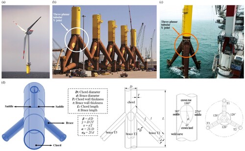
Jacket and tripod structures are steel space frames composed of welded circular hollows section (CHS) members also called tubulars. They are commonly used in offshore industry as the substructure of fixed offshore oil/gas platforms and offshore wind turbines (OWTs) as shown in Figure 1(a). The connection between the tubulars in which the prepared ends of brace members are welded onto the undisturbed surface of a chord member is called a tubular joint (Figure 1(b,c)).

Figure 1. (a) A typical offshore wind turbine with tripod substructure in service, (b) Tripod substructures during the fabrication, (c) A tripod substructure during the installation, (d) Geometrical notation for a three-planar tubular Y-joint (This figure is available in colour online).

The local joint flexibility (LJF) which is an intrinsic feature of a tubular joint is one of the factors affecting the global static and dynamic responses of an offshore structure. The LJF increases the deflections, redistributes the nominal stresses, reduces the buckling loads, and changes the natural frequencies of the structure (Bouwkamp et al. 1980; UEG 1985; Gao et al. 2013). For example, analysis of a jacket platform considering the local flexibility of the joints results in higher primary natural period of vibration and lower base shear compared to the case in which the joints are assumed to be rigid. These facts imply that the conventional procedures for the analysis and design of tubular structures with the assumption that the tubular joints are rigid may not be accurate enough, especially for unstiffened joints. Hence, it is necessary to determine the local joint flexibility for commonly used tubular joints.

The primary factors affecting the LJF are the joint type, its geometrical properties, and brace loading type. In order to relate the behaviour of a tubular joint to its geometrical characteristics, a set of dimensionless geometrical parameters including α, α_B, β, γ, and τ, defined in Figure 1(d), is commonly used.

UEG (1985) and DNV (1977) have provided parametric equations to determine the LJF for tubular T-/Y-joints. The UEG guidelines do not clearly define the range of applicability; and the DNV equations are based on a limited number of FE analyses. Efthymiou (1985) developed a set of equations for T-, Y-, and K-joints subjected to in-plane bending (IPB) and out-of-plane bending (OPB) loads by numerical analysis. The database was limited to 12 T-, 3 Y-, and 5 K-joints, 5 of which were partially overlapped.

Fessler et al. (1986a, 1986b) measured the local deformation of the chord wall subjected to basic loadings within the elastic range based on 27 models and derived a set of parametric equations for both T-/Y- and K-joints. However, their experimental models were made from araldite instead of steel; and they had relatively small scale. Ueda et al. (1990) proposed a set of equations to predict the LJF under the axial and IPB loads based on FE analysis of 11 T-joint models. The results amended and improved the accuracy and maintained the simplicity of numerical computation as well. However, the validity range of geometrical parameters for these equations was very limited in terms of brace-to-chord diameter ratio, which was restricted to 0.35−0.55.

Chen et al. (1990) determined the LJF of T-, Y-, and K-joints. By using the semi-analytical approach, Chen et al. (1993) and Hoshyari and Kohoutek (1993) quantified the LJF for simple gap K- and T-/Y-joints, respectively. Buitrago et al. (1993) provided the methodology as well as the parametric equations for computing the LJF in gap and partially overlapped joints based on the FE analysis. Chen and Zhang (1996) studied the stress distribution in space frames with the consideration of local flexibility of multiplanar tubular joints.

Hu et al. (1993) and Golafshani et al. (2013) proposed equivalent elements representing the local flexibility of tubular joints in structural analysis of offshore platforms. Gao et al. (2013, 2014) and Gao and Hu (2015) proposed parametric equations to predict the LJF in completely overlapped tubular joints subjected to axial, IPB, and OPB loadings, respectively.

Ahmadi and Ziaei Nejad (2017a, 2017b, 2017c) developed a set of parametric equations to determine the LJF factor (f_LJF), defined in Sect. 2.1, in two-planar tubular DK-joints subjected to axial, IPB, and OPB loadings, respectively. They indicated that the effect of multi-planarity on the LJF can be significant and consequently the use of the equations already available for uniplanar joints to calculate the LJF in multi-planar joints may lead to highly under-/over-predicting results.

Ahmadi and Mayeli (2018, 2019) derived the probability density functions (PDFs) governing the f_LJF in tubular DK-joints subjected to eight types of bending moment loads including four types of IPB and four types of OPB loadings. Developed PDFs are useful for the reliability analysis of offshore jacket structures in order to calculate the probability of structural failure.

Nassiraei (2019) studied the local joint flexibility of tubular X-joints reinforced with collar plates subjected to axial loading. Geometrical effects on the LJF of tubular T/Y-joints with doubler and collar plates were investigated by Nassiraei (2020a, 2020b). Nassiraei and Rezadoost (2021a) investigated the local joint flexibility of tubular T/Y-joints retrofitted with GFRP under in-plane bending moment. Nassiraei and Rezadoost (2021b) studied the local joint flexibility of tubular X-joints stiffened with external ring or external plates.

Ahmadi and Mohammadpourian Janfeshan (2021) and Ahmadi and Akhtegan (2022) investigated the effects of geometrical parameters on the LJF of offshore two- and three-planar tubular T-joints, respectively. Nassiraei and Yara (2022a, 2022b) examined the local joint flexibility of tubular K-joints reinforced with external plates under the IPB and OPB moment loadings.

The above discussion on the previous investigations of the LJF indicates that the LJF for uniplanar tubular joints such as T-/Y-, X-, and K-joints due to basic load cases has been extensively studied; based on which extensive parametric equations have been derived. However, for multi-planar tubular joints which cover the majority of practical applications, the research works in terms of the LJF are very limited mainly due to the more complexities involved in the modelling.

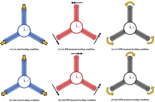
In the present paper, results of a parametric study carried out on the LJF of three-planar tubular Y-joints subjected to six types of axial, IPB moment, and OPB moment loadings (Figure 2) are presented and discussed. A total of 81 FE models were used to study the effects of the three-planar Y-joint’s geometrical parameters on the f_LJF. Generated FE models were validated based on the existing experimental data and parametric equations. The f_LJF values in three-planar and uniplanar Y-joints were compared; and the FE results were used to derive a new parametric equation for the prediction of the f_LJF in axially loaded three-planar Y-joints. The proposed equation was checked against the acceptance criteria recommended by the UK DoE (1983) and hence can be reliably used for the analysis and design of tubular joints in substructures of offshore wind turbines.

Figure 2. Studied axial, IPB moment, and OPB moment loading conditions (This figure is available in colour online).

2. Methodology

2.1. Calculation of the f_LJF

2.1.1. Axial loading

The LJF of an axially loaded tubular joint is defined as the displacement attributed to the local chord wall deformation due to a unit applied load. It measures the distortion of the CHS which is an oval shape under the axial loading without considering the beam bending movement (Gao et al. 2013).

The LJF of a tubular joint under the axial loading can be calculated as follows: (1) $\mathrm{LJF}=\left({\delta }_{\mathrm{AX}}/P_{\mathrm{AX}}\right)\sin \theta$(1) where θ is the brace inclination angle (Figure 1(d)), P_AX is the axial load of the brace, and δ_AX is the displacement caused only by chord wall deformation, in which overall bending deflection of the chord acting as a beam must be excluded.

Since the intersection of the brace and chord members is a space curve, for the purpose of actual calculation in an FE model, ${\delta }_{\mathrm{AX}}$ can be expressed as the average local displacement of the joint normal to the chord axis: (2) ${\delta }_{\mathrm{AX}}={\displaystyle \frac{\left({\delta }_1-{{\delta }^{\mathrm{\prime }}}_1\right)+\left({\delta }_2-{{\delta }^{\mathrm{\prime }}}_2\right)+\left({\delta }_3-{{\delta }^{\mathrm{\prime }}}_3\right)+\left({\delta }_4-{{\delta }^{\mathrm{\prime }}}_4\right)}{4}}$(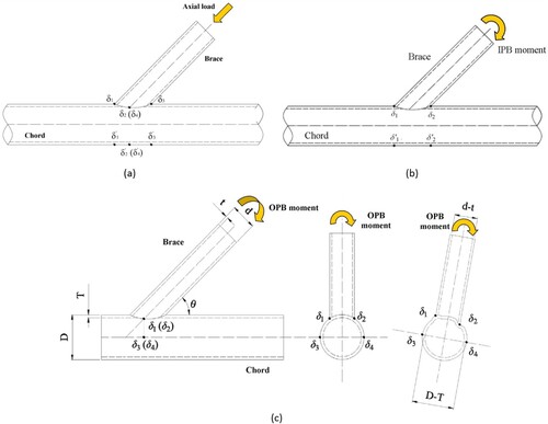2) where δ₁, δ₂, δ₃, and δ₄ are the displacements at the crown toe, crown heel, and two saddle positions measured perpendicular to the chord axis; and δ'₁, δ'₂, δ'₃, and δ'₄ are the bending deflections that can be determined by simple beam theory. Saddle, crown toe, and crown heel positions are shown in Figure 1(d).

According to Gao et al. (2013, 2014), bending deflections in an FE model can be reasonably approximated by the displacements at the bottom of the chord member corresponding to δ₁, δ₂, δ₃, and δ₄, respectively (Figure 3(a)). The reader is referred to Chen et al. (1990) for the details of deriving Equations (1) and (2).

Figure 3. Positions for the deformation measurement to determine the f_LJF in a tubular joint subjected to (a) axial loading, (b) IPB moment loading, (c) OPB moment loading (This figure is available in colour online).

In order to relate the local joint flexibility to dimensionless geometrical parameters of the joint, a dimensionless coefficient called the local joint flexibility factor (f_LJF) is defined. Under the axial loading, the f_LJF is the LJF multiplied by ED: (3) $f_{\mathrm{LJF}}=\left({\delta }_{\mathrm{AX}}/P_{\mathrm{AX}}\right)\mathrm{EDsin}\theta$(3) where D is the chord diameter and E is the Young’s modulus.

2.1.2. IPB moment loading

To determine the LJF factor under the brace IPB moment loading, the rotation of the joint due to the overall displacement should be omitted from the total measured rotation. In an FE model, the local rotation at the joint can be directly measured without considering the beam bending movement. It measures the distortion of the circular cross section which is an oval shape under the IPB load. The LJF of a tubular joint under the IPB loading can be defined as (Gao et al. 2014): (4) $\mathrm{LJF}={\varphi }_{\mathrm{IPB}}/M_{\mathrm{IPB}}$(4) where M_IPB is the brace IPB moment and ${\varphi }_{\mathrm{IPB}}$ is the joint local rotation expressed as: (5) ${\varphi }_{\mathrm{IPB}}={\displaystyle \frac{\left({\delta }_2-{{\delta }^{\mathrm{\prime }}}_2\right)-\left({\delta }_1-{{\delta }^{\mathrm{\prime }}}_1\right)}{d-t}\sin \theta }$(5) where d is the brace diameter; t is the brace wall thickness; θ is the angle between the chord and brace members; δ₁ and δ₂ are the respective deformations at the crown toe and heel positions measured perpendicular to the chord axis as shown in Figure 3(b); and δ'₁ and δ'₂ are the deformations at the bottom of the chord corresponding to δ₁ and δ₂, respectively.

Under the IPB moment loading, the f_LJF is the LJF multiplied by ED³: (6) $f_{\mathrm{LJF}}={\displaystyle \frac{{\varphi }_{\mathrm{IPB}}}{M_{\mathrm{IPB}}}E{D}^3}$(6) where D is the chord diameter and E is the Young’s modulus.

2.1.3. OPB moment loading

The LJF of a tubular joint under the OPB loading can be defined as (Gao and Hu 2015): (7) $\mathrm{LJF}={\varphi }_{\mathrm{OPB}}/M_{\mathrm{OPB}}$(7) where M_OPB is the brace OPB moment and ${\varphi }_{\mathrm{OPB}}$ is the joint local rotation expressed as: (8) ${\varphi }_{\mathrm{OPB}}={\displaystyle \frac{{\delta }_2-{\delta }_1}{d-t}\sin \theta -{\displaystyle \frac{{\delta }_4-{\delta }_3}{D-T}}}$(8) where D and d are the chord and brace diameters respectively; T and t are the chord and brace wall thicknesses respectively; θ is the brace inclination angle; δ₁ and δ₂ are the respective deformations at both saddles measured in the direction of brace axis; and δ₃ and δ₄ are the deformations at the side face of the chord corresponding to δ₁ and δ₂, respectively (Figure 3(c)).

Under the OPB moment loading, the f_LJF is the LJF multiplied by ED³: (9) $f_{\mathrm{LJF}}={\displaystyle \frac{{\varphi }_{\mathrm{OPB}}}{M_{\mathrm{OPB}}}E{D}^3}$(9)

2.2. FE modelling and analysis of three-planar tubular Y-joints to calculate the f_LJF

FE-based software package ANSYS was used in the present research for the modelling and analysis of three-planar tubular Y-joints subjected to axial loading in order to determine the f_LJF values for the parametric study and design formulation. This section presents the details of FE modelling and analysis.

2.2.1. Modelling of the weld profile

One of the factors which affects the accuracy of the f_LJF results is the modelling of the weld profile. In the present research, the welding size along the brace-to-chord intersection satisfies the AWS D 1.1 (2002) specifications. The weld sizes at the saddle, crown toe, and crown heel positions can be determined as follows: (10) $\begin{array}{rl}& H_w\left(\mathrm{mm}\right)=0.85t\left(\mathrm{mm}\right)+4.24\\ & L_w={\displaystyle \frac{t}{2}\left[{\displaystyle \frac{{135}^{\circ }-\psi (\mathrm{deg}.)}{{45}^{\circ }}}\right]}\\ & \psi =\{\begin{array}{c}{180}^{\circ }-{\cos }^{-1}\text{β}(\mathrm{deg}.)\\ {180}^{\circ }-\theta (\mathrm{deg}.)\\ \theta (\mathrm{deg}.)\end{array}\begin{array}{c}\\ \\ \end{array}\begin{array}{c}\\ \\ \end{array}\begin{array}{c}\mathrm{Saddle}\\ \mathrm{Crowntoe}\\ \mathrm{Crownheel}\end{array}\end{array}$(10)

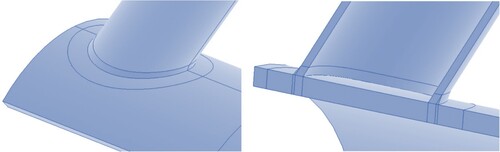
The parameters used in Equation (10) are defined in Figure 4. As an example, the weld profile generated for a sample joint model (α = 8, τ = 0.7, β = 0.3, γ = 12, θ = 60°) is shown in Figure 5. For details of the weld profile modelling according to AWS D 1.1 (2002) specifications, the reader is referred to Lie et al. (2001).

Figure 4. Weld dimensions: (a) Saddle position, (b) Crown toe position, (c) Crown heel position (This figure is available in colour online).

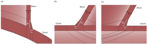
Figure 5. The weld profile generated for a sample joint model (α = 8, τ = 0.7, β = 0.3, γ = 12, θ = 60°) (This figure is available in colour online).

2.2.2. Application of boundary conditions

Chord end fixity condition in tubular joints of offshore structures ranges from almost fixed to almost pinned with generally being closer to almost fixed (Efthymiou 1988). In the view of the fact that the effect of the chord end restraints on the stress distribution at the brace/chord intersection is only significant for joints with α < 8 and high β and γ values (Smedley and Fisher 1991; Morgan and Lee 1998), which do not commonly occur in practice, both chord ends were assumed to be fixed, with the corresponding nodes restrained. For a joint with the brace member of sufficient length, the brace end fixity imposes marginal effects on the joint strength (Choo et al. 2006). The sufficient brace length is discussed in Sect. 2.3. In the present research, no restraint was applied to the upper end of brace members.

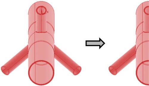
Application of symmetric and antisymmetric boundary conditions is beneficial in order to reduce the computational time. Due to the symmetry in geometry and loading of the joint, only ½ of the entire three-planar tubular Y-joint is required to be modelled subjected to the 1st and 2nd axial load cases, as well as the 1st and 2nd IPB moment loading conditions. Similarly, due to the symmetry in geometry and antisymmetry in loading, again only half of the entire three-planar joint should be modelled under the 1st OPB moment loading condition. However, a full three-planar tubular Y-joint must be modelled subjected to the 2nd OPB moment loading condition (Figure 6). Appropriate symmetric and antisymmetric boundary conditions were defined for the nodes located on the symmetry and antisymmetry planes.

Figure 6. Half of the entire three-planar Y-joint that is required to be modelled under the 1st and 2nd axial, 1st and 2nd IPB moment, and 1st OPB moment loading conditions (This figure is available in colour online).

2.2.3. Mesh generation and analysis

In order to model the chord, braces, and the weld profiles, ANSYS brick element type SOLID185 was used. This element has compatible displacements and is well-suited to model curved boundaries. The element is defined by eight nodes having three degrees of freedom per node and may have any spatial orientation. Using this type of 3-D brick elements, the weld profile can be modelled as a sharp notch. This method will produce more accurate and detailed stress distribution near the intersection in comparison with a simple shell analysis.

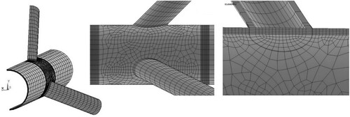
To guarantee the mesh quality, a sub-zone mesh generation method was used during the FE modelling. In this method, the entire structure is divided into several different zones according to the computational requirements. The mesh of each zone is generated separately and then the mesh of entire structure is produced by merging the meshes of all the sub-zones. This method can easily control the mesh quantity and quality and avoid badly distorted elements. The mesh generated by this method for a three-planar Y-joint is shown in Figure 7.

Figure 7. Generated mesh by the sub-zone scheme.

In order to make sure that the results of the FE analysis are not affected by the inadequate quality or the size of the generated mesh, convergence test was conducted and meshes with different densities were used in this test, before generating the 81 models. Based on the results of convergence test, the number of elements through the chord and brace thickness was 1; the number of elements on the surface, base, and back of the weld profile was 2; and the number of elements along ½ of the entire brace-to-chord intersection was selected to be 22.

The static analysis of linearly elastic type is suitable for the prediction of LJF in tubular joints (Gao et al. 2013, 2014). The Young’s modulus and Poisson’s ratio were taken to be 207 GPa and 0.3, respectively.

2.2.4. Verification of the FE model

The accuracy of FE results to determine the f_LJF in tubular joints should be validated using the experimental test results. To the best of the authors’ knowledge, there is no experimental/FE database of f_LJF for three-planar tubular Y-joints currently available in the literature. Considering this issue, in order to verify the FE model used in the present study, a set of uniplanar Y-joints were modelled (Figure 8) and the f_LJF values obtained from these models subjected to axial, IPB moment, and OPB moment loadings were compared with the experimental results of Fessler et al. (1986b) and values predicted by Fessler et al. (1986b) equations. Geometrical properties of the validating Y-joints have been presented in Table 1.

Figure 8. (a) A validating Y-joint FE model developed to compare its results with available experimental data and results of parametric equations proposed by Fessler et al. (1986b), (b) ½ of the entire validating FE model required to be generated in order to reduce the computational time (This figure is available in colour online).

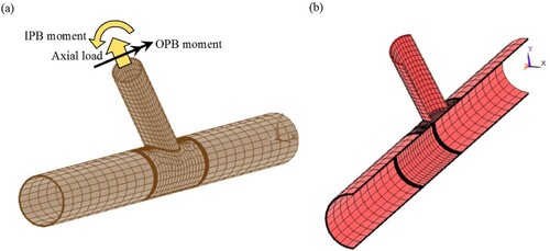
Table 1. Geometrical properties of the uniplanar tubular Y-joints used for the verification of FE models.

Joint ID	Dimensions (mm)						Parameters					θ
	D	T	L	d	t	l	τ	β	γ	α	αB
Y1	132	6.6	813	44	2.6	250	0.39	0.33	15	12.32	11.36	50°
Y2	132	6.6	813	70	2.6	225	0.39	0.53	15	12.32	6.43	50°
Y3	132	6.6	813	100	3.2	200	0.48	0.76	15	12.32	4.00	50°

The procedure of geometrical modelling (introducing the chord, braces, and weld profiles), the mesh generation method (including the selection of the element type and size), the analysis type, and the method of f_LJF calculation are the same for the validating uniplanar Y-joint models and the three-planar Y-joints used in the present research for the parametric study. Hence, the verification of the f_LJF values derived from the validating FE models with available corresponding experimental/equation-predicted values lends some support to the validity of the f_LJF values derived from the three-planar Y-joint FE models.

Results of the FE validation process, presented in Table 2, indicate that there is a good agreement between the results of previous studies and the predictions of the validating FE model. According to Table 2, the average difference between the f_LJF of the validating FE model and the experimental results of Fessler et al. (1986b) is 11.3%; while the average difference between the results of the validating FE model and the equations proposed by Fessler et al. (1986b) is 6.2%. Hence, generated FE models can be considered to be accurate enough to provide valid results.

Table 2. Results of the FE model verification based on available experimental data and parametric equations.

Loading type	Joint ID	fLJF			(a)–(b) difference (%)	(a)–(c) difference (%)
		(a) Present FE model	(b) Fessler et al. (1986b) experiment	(c) Fessler et al. (1986b) equation
Axial	Y1	205	223	217	8.1	5.6
IPB	Y2	2180	2361	2417	7.6	9.8
OPB	Y3	350	296	339	18.2	3.2

2.3. Details of parametric study

To study the effects of non-dimensional geometrical parameters on the f_LJF values in three-planar tubular Y-joints subjected to the 2nd axial loading condition (Figure 2(b)), 81 models were generated and analyzed using the FE-based software package, ANSYS. The reason behind selecting this specific loading condition for the parametric study is fully discussed in Sect. 3.1.

Values assigned to the parameters β, γ, τ, and α have been presented in Table 3. These values cover the practical ranges of dimensionless parameters typically found in tubular joints of offshore jacket structures. The brace length has no effect on the results when the parameter α_B is greater than a critical value (Chang and Dover 1999). According to Chang and Dover (1996), this critical value is about 6. In the present study, in order to avoid the effect of short brace length, a realistic value of α_B = 8 was assigned to all joints. Ahmadi and Ziaei Nejad (2017a) and Ahmadi and Mohammadpourian Janfeshan (2021) showed that the parameter τ has no considerable effect on the f_LJF values. Hence, a typical value of τ = 0.7 was selected for all the Y-joints in the present research. Results of parametric study are presented and discussed in Sect. 3.2.

Table 3. Values assigned to each dimensionless parameter.

Parameter	Definition	Value(s)
β	d/D	0.3, 0.45, 0.6
γ	D/2T	12, 18, 24
θ	Brace inclination angle	30°, 45°, 60°
α	2L/D	8, 16, 24
αB	2l/d	8
τ	t/T	0.7

The 81 generated models span the following ranges of dimensionless geometrical parameters: (11) $\begin{array}{rl}& 0.3\le \text{β}\le 0.6\\ & 12\le \gamma \le 24\\ & {30}^{\circ }\le \theta \le {60}^{\circ }\\ & 8\le \alpha \le 24\end{array}$(11)

2.4. Development of a parametric design equation

In order to calculate the f_LJF values for three-planar tubular Y-joints subjected to axial loading, a new parametric equation is proposed in the present paper. Results of multiple nonlinear regression analyses performed by SPSS were used to develop this parametric f_LJF formula. Values of dependent variable (i.e. f_LJF) and independent variables (i.e. β, γ, θ, and α) constitute the input data imported in the form of a matrix. Each row of this matrix involves the information about the f_LJF value of a three-planar tubular Y-joint having specific geometrical properties. When the dependent and independent variables are defined, a model expression must be built with defined parameters. Parameters of the model expression are unknown coefficients and exponents. The researcher must specify a starting value for each parameter, preferably as close as possible to the expected final solution. Poor starting values can result in failure to converge or in convergence on a solution that is local (rather than global) or is physically impossible. Various model expressions must be built to derive a parametric equation having a high coefficient of determination (R²). Developed parametric equation along with a discussion on its applicability is presented in Sect. 3.3.

3. Results and discussion

3.1. The effect of multi-planarity on the f_LJF values subjected to different types of loading

In order to investigate the multi-planarity effects on the f_LJF values subjected to the axial, IPB moment, and OPB moment loading conditions, nine uniplanar Y-joints were generated and the f_LJF values of these joints were compared with the f_LJF values of the corresponding three-planar Y-joints. Geometrical properties of these joints are given in Table 4.

Table 4. Geometrical properties of the uniplanar and three-planar tubular Y-joints used to investigate the multi-planarity effects on the f_LJF values subjected to the six studied loading conditions.

Joint ID	D (mm)	T (mm)	L (mm)	d (mm)	t (mm)	l (mm)	β	γ	θ	α	αB	τ
YJ1	500	20.83	4000	225	14.6	900	0.45	12	30°	16	8	0.7
YJ2	500	20.83	4000	225	14.6	900	0.45	12	45°	16	8	0.7
YJ3	500	20.83	4000	225	14.6	900	0.45	12	60°	16	8	0.7
YJ4	500	14	4000	225	9.8	900	0.45	18	30°	16	8	0.7
YJ5	500	14	4000	225	9.8	900	0.45	18	45°	16	8	0.7
YJ6	500	14	4000	225	9.8	900	0.45	18	60°	16	8	0.7
YJ7	500	10	4000	225	7	900	0.45	24	30°	16	8	0.7
YJ8	500	10	4000	225	7	900	0.45	24	45°	16	8	0.7
YJ9	500	10	4000	225	7	900	0.45	24	60°	16	8	0.7

3.1.1. Axial loading

In order to study the effect of multi-planarity on the f_LJF values under the 1st and 2nd types of axial loading (Figure 2(a,b)), values of the f_LJF in nine multi-planar tubular Y-joints were compared with the f_LJF values obtained from the corresponding uniplanar Y-joints under the two considered axial load cases. Results summarised in Table 5 show that the f_LJF value in a three-planar Y-joint under the 1st axial loading condition is smaller than the corresponding f_LJF value in a uniplanar Y-joint; where, on an average basis, the three-planar to uniplanar f_LJF ratio is 0.88. Under the 2nd axial loading condition, the f_LJF value in a three-planar Y-joint is much bigger than the corresponding f_LJF value in a uniplanar Y-joint; where, on average, the three-planar to uniplanar f_LJF ratio is 2.09.

Table 5. Comparison of the f_LJF values in uniplanar and three-planar Y-joints subjected to the axial load cases.

Joint ID	Loading condition	fLJF Value
		Uniplanar joint	Three-planar joint	Difference (%)
YJ1	1st axial load case (Figure 2(a))	18.9	14.97	21.16
	2nd axial load case (Figure 2(b))		38.1	50.39
YJ2	1st axial load case (Figure 2(a))	40.3	30.5	24.3
	2nd axial load case (Figure 2(b))		82.6	51.2
YJ3	1st axial load case (Figure 2(a))	127.5	126.7	0.7
	2nd axial load case (Figure 2(b))		264	51.89
YJ4	1st axial load case (Figure 2(a))	80.26	63.1	21.38
	2nd axial load case (Figure 2(b))		156	48.5
YJ5	1st axial load case (Figure 2(a))	171.7	148.3	13.4
	2nd axial load case (Figure 2(b))		347	50.72
YJ6	1st axial load case (Figure 2(a))	259.6	232	10.42
	2nd axial load case (Figure 2(b))		527	50.85
YJ7	1st axial load case (Figure 2(a))	122.5	115.9	5.7
	2nd axial load case (Figure 2(b))		255	52.15
YJ8	1st axial load case (Figure 2(a))	211	229	7.8
	2nd axial load case (Figure 2(b))		533	60.4
YJ9	1st axial load case (Figure 2(a))	437.3	361	17.39
	2nd axial load case (Figure 2(b))		901	51.5

Hence, it can be concluded that for axially loaded three-planar Y-joints, the parametric formulas of simple uniplanar Y-joints are not applicable for the f_LJF prediction, since such formulas may lead to highly under-predicting results. Consequently, developing a set of specific parametric equations for the f_LJF calculation in three-planar Y-joints has practical value.

3.1.2. IPB loading

To study the effect of multi-planarity on the f_LJF values under the 1st and 2nd types of IPB loading (Figure 2(c,d)), values of the f_LJF in nine multi-planar tubular Y-joints were compared with the f_LJF values obtained from the corresponding uniplanar Y-joints under the two considered IPB load cases. Results are presented in Table 6 showing that, under both considered IPB moment loadings, the f_LJF values in three-planar Y-joints are smaller than the corresponding f_LJF values in uniplanar Y-joints. On an average basis, the differences between the three-planar and uniplanar f_LJF values for the 1st and 2nd IPB load cases are 11.8% and 77.7%, respectively.

Table 6. Comparison of the f_LJF values in uniplanar and three-planar Y-joints subjected to the IPB load cases.

Joint ID	Loading condition	fLJF Value
		Uniplanar joint	Three-planar joint	Difference (%)
YJ1	1st IPB load case (Figure 2(c))	7878	7254	7.9
	2nd IPB load case (Figure 2(d))		1098	86
YJ2	1st IPB load case (Figure 2(c))	8125	7852	3.36
	2nd IPB load case (Figure 2(d))		1125	86.1
YJ3	1st IPB load case (Figure 2(c))	8651	8001	7.5
	2nd IPB load case (Figure 2(d))		1642	81
YJ4	1st IPB load case (Figure 2(c))	9125	8247	9.6
	2nd IPB load case (Figure 2(d))		1896	79.22
YJ5	1st IPB load case (Figure 2(c))	9862	8574	13.06
	2nd IPB load case (Figure 2(d))		2198	77.7
YJ6	1st IPB load case (Figure 2(c))	10081	8842	12.2
	2nd IPB load case (Figure 2(d))		2531	74.9
YJ7	1st IPB load case (Figure 2(c))	10958	9011	17.7
	2nd IPB load case (Figure 2(d))		2994	72.6
YJ8	1st IPB load case (Figure 2(c))	11023	9200	16.5
	2nd IPB load case (Figure 2(d))		3111	71.7
YJ9	1st IPB load case (Fig. 2c)	11855	9655	18.55
	2nd IPB load case (Figure 2(d))		3487	70.5

3.1.3. OPB loading

To investigate the effect of multi-planarity on the f_LJF values under the 1st and 2nd types of OPB loading (Figure 2(e,f)), values of the f_LJF in nine multi-planar tubular Y-joints were compared with the f_LJF values obtained from the corresponding uniplanar Y-joints under the two studied OPB load cases. Results are presented in Table 7 indicating that, under both considered OPB moment loadings, the f_LJF values in three-planar Y-joints are bigger than the corresponding f_LJF values in uniplanar Y-joints. However, the amount of the difference between the three-planar and uniplanar f_LJF values is not large; where, on an average basis, the difference between the three-planar and uniplanar f_LJF values is 10.2%.

Table 7. Comparison of the f_LJF values in uniplanar and three-planar Y-joints subjected to the OPB load cases.

Joint ID	Loading condition	fLJF value
		Uniplanar joint	Three-planar joint	Difference (%)
YJ1	1st OPB load case (Figure 2(e))	6638	6821	2.7
	2nd OPB load case (Figure 2(f))		7568	12.28
YJ2	1st OPB load case (Figure 2(e))	6218	6698	7.1
	2nd OPB load case (Figure 2(f))		7089	12.28
YJ3	1st OPB load case (Figure 2(e))	5897	6254	5.7
	2nd OPB load case (Figure 2(f))		6480	9
YJ4	1st OPB load case (Figure 2(e))	5321	5897	9.7
	2nd OPB load case (Figure 2(f))		6142	13.3
YJ5	1st OPB load case (Figure 2(e))	5012	5606	10.5
	2nd OPB load case (Figure 2(f))		5861	14.48
YJ6	1st OPB load case (Figure 2(e))	4981	5296	6
	2nd OPB load case (Figure 2(f))		5500	9.4
YJ7	1st OPB load case (Figure 2(e))	4456	4958	10.12
	2nd OPB load case (Figure 2(f))		5023	11.28
YJ8	1st OPB load case (Figure 2(e))	4189	4765	12
	2nd OPB load case (Figure 2(f))		4875	14
YJ9	1st OPB load case (Figure 2(e))	3847	4294	10.4
	2nd OPB load case (Figure 2(f))		4456	13.6

3.1.4. Critical loading condition

Since the increase of the LJF increases the deflections and reduces the buckling load as well as the primary natural frequency of the structure, biggest values of the f_LJF are of real concern for the structural design applications and smaller f_LJF values merely mean that the considered tubular joint can be safely assumed to be rigid. Hence, according to Sects. 3.1.1−3.1.3, the only loading case under which the f_LJF values should be individually studied with the aim of investigating the effects of geometrical parameters and the development of design equations is the 2nd type of axial loading (Figure 2(b)).

3.2. Effects of geometrical parameters of the joint on the f_LJF values

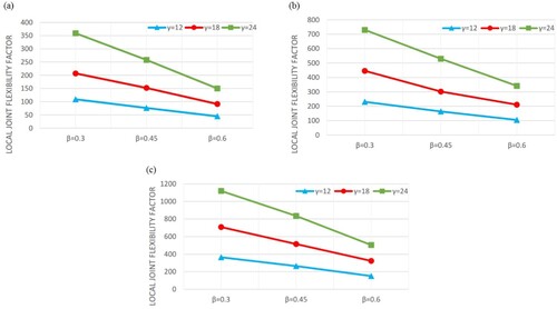
3.2.1. The effect of the β on the f_LJF values

The parameter β is the ratio of the brace diameter to the chord diameter. Hence, provided that the chord diameter remains constant, the increase of the β results in the increase of the brace diameter. Figure 9 demonstrates the change of the f_LJF, under the 2nd axial loading condition, due to the change in the value of the β and the interaction of this parameter with the γ. It can be seen that the increase of the β results in the decrease of the f_LJF. The reason is that the increase of the β leads to the increase of the joint stiffness (due to the increase of the chord diameter) which consequently results in the decrease of the joint deflection; and hence, according to Equation (3), the decrease of the f_LJF. As can be observed in Figure 9, this conclusion is independent from the values of other geometrical parameters. It can also be seen that the increase of the γ leads to increasing the slope of the f_LJF decrement curve due to the increase of the β. In other words, in joints with bigger values of the γ, the increase of the β results in more drastic decrease of the f_LJF.

Figure 9. The effect of the β on the f_LJF values and its interaction with the γ under the 2nd axial loading condition (τ = 0.7, α = 24): (a) θ = 30°, (b) θ = 45°, (c) θ = 60° (This figure is available in colour online).

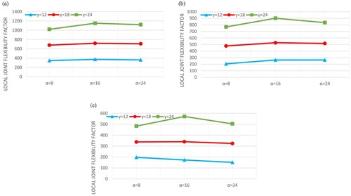
3.2.2. The effect of the α on the f_LJF values

The parameter α is the ratio of the length to the radius of the chord. Hence, the increase of the α in models having constant value of the chord diameter means the increase of the chord length. Figure 10 shows the change of the f_LJF due to the change in the value of the α and the interaction of this parameter with the γ under the 2nd axial loading condition. Results showed that the change of the f_LJF as a function of the α does not exactly follow a regular pattern. However, the amount of the change in the f_LJF values due to the change of the α is usually not significant.

Figure 10. The effect of the α on the f_LJF values and its interaction with the γ under the 2nd axial loading condition (τ = 0.7, θ = 60°): (a) β = 0.3, (b) β = 0.45, (c) β = 0.6 (This figure is available in colour online).

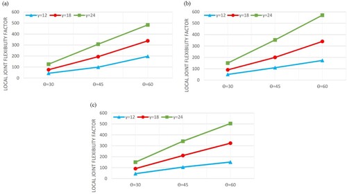
3.2.3. The effect of the θ on the f_LJF values

Figure 11 depicts the change of the f_LJF values as a function of the brace inclination angle θ and the interaction of this parameter with the γ under the 2nd axial loading condition. It can be seen that the increase of the θ leads to the increase of the f_LJF. As can be observed in Figure 11, this conclusion is independent from the values of other geometrical parameters. It can also be seen that the increase of the γ leads to increasing the slope of the f_LJF increment curve due to the increase of the θ. In other words, in joints with bigger values of the γ, the increase of the θ results in more drastic increase of the f_LJF.

Figure 11. The effect of the θ on the f_LJF values and its interaction with the γ under the 2nd axial loading condition (τ = 0.7, α = 24): (a) β = 0.3, (b) β = 0.45, (c) β = 0.6 (This figure is available in colour online).

3.2.4. The effect of the γ on the f_LJF values

The parameter γ is the ratio of the section radius to wall thickness of the chord. Hence, provided that the chord diameter remains constant, the increase of the γ means the decrease of the chord thickness. It is evident from Figures 9–11 that the increase of the γ leads to the increase of the f_LJF. The reason is that the increase of the γ leads to the decrease of the joint stiffness (due to the decrease of the chord wall thickness) which consequently results in the increase of the joint deflection; and hence, according to Equation (3), the increase of the f_LJF. This conclusion does not depend on the values of other geometrical parameters.

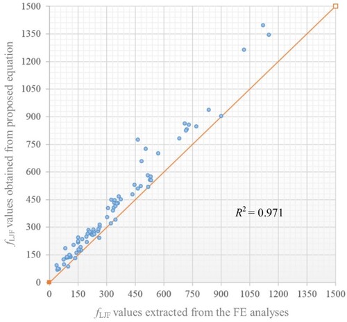
3.3. Proposed parametric equation for the calculation of the f_LJF

After performing a large number of nonlinear analyses, as described in Sect. 2.4, following parametric equation is proposed for the calculation of the f_LJF values in three-planar tubular Y-joints subjected to the 2nd axial loading condition (Figure 2(b)): (12) $f_{\mathrm{LJF}}=0.001{\theta }^{1.697}\exp \left[2.288\left(1+{\text{β}}^{-0.314}+{\gamma }^{0.297}+{\alpha }^{0.036}\right)\right]$(12) A quite high value of 0.971 was obtained for the coefficient of determination (R²) indicating the accuracy of the fit. The validity ranges of dimensionless geometrical parameters for the developed equation have been given in Equation (11). The 1st axial loading condition as well as the IPB and OPB moment loading conditions were completely omitted during the equation development phase due to the reasons discussed in Sect. 3.1.4.

Figure 12 compares the f_LJF values predicted by the proposed equation with the f_LJF values extracted from FE analyses. It can be seen that there is a very good agreement between the results of the proposed equation and numerically computed values.

Figure 12. Comparison of 81 f_LJF values calculated by the proposed equation (Equation (12)) with the corresponding f_LJF values extracted from the FE analyses (This figure is available in colour online).

The UK Department of Energy (DoE) (1983) recommends the following assessment criteria regarding the applicability of the parametric equations (P/R stands for the ratio of the predicted f_LJF from proposed equation to the recorded f_LJF from FE analysis):

• For a given dataset, if % f_LJF values under-predicting $\le$ 25%, i.e. [%P/R < 1.0] $\le$ 25%, and if % f_LJF values considerably under-predicting $\le$ 5%, i.e. [%P/R < 0.8] $\le$ 5%, then accept the equation. If, in addition, the percentage f_LJF values considerably over-predicting $\le$ 50%, i.e. [%P/R > 1.5] $\ge$50%, then the equation is regarded as generally conservative.

• If the acceptance criteria is nearly met i.e. 25% < [%P/R < 1.0] $\le$ 30%, and/or 5% < [%P/R < 0.8] $\le$ 7.5%, then the equation is regarded as borderline and engineering judgment must be used to determine acceptance or rejection.

• Otherwise reject the equation as it is too optimistic.

In view of the fact that for a mean fit equation, there is always a large percentage of under-prediction, the requirement for joint under-prediction, i.e. P/R < 1.0, can be completely removed in the assessment of parametric equations (Bomel Consulting Engineers 1994). Assessment results according to the UK DoE (1983) criteria are presented in Table 8 showing that Equation (12) satisfies the criteria, and hence it can be reliably used for the design of three-planar tubular Y-joints.

Table 8. Results of f_LJF equation assessment according to the UK DoE (1983) acceptance criteria.

Proposed equation	UK DoE conditions		Decision
	%P/R < 0.8	%P/R > 1.5
Equation (12)	0% < 5% OK.	12.34% < 50% OK.	Accept

6. Conclusions

In order to study the effects of geometrical characteristics of three-planar tubular Y-joints on the LJF factor (f_LJF), 81 FE models were generated and analyzed subjected to six types of axial, in-plane bending (IPB) moment, and out-of-plane bending (OPB) moment loadings. Results can be summarised as follows.

The f_LJF value in a three-planar Y-joint under the 1st axial loading condition is smaller than the corresponding f_LJF value in a uniplanar Y-joint; where, on an average basis, the three-planar to uniplanar f_LJF ratio is 0.88. Under the 2nd axial loading condition, the f_LJF value in a three-planar Y-joint is much bigger than the corresponding f_LJF value in a uniplanar Y-joint; where, on average, the three-planar to uniplanar f_LJF ratio is 2.09. Hence, it can be concluded that for axially loaded three-planar Y-joints, the parametric formulas of simple uniplanar Y-joints are not applicable for the f_LJF prediction, since such formulas may lead to highly under-predicting results. Consequently, developing a set of specific parametric equations for the f_LJF calculation in three-planar Y-joints has practical value.

Under both considered IPB moment loadings, the f_LJF values in three-planar Y-joints are smaller than the corresponding f_LJF values in uniplanar Y-joints. On an average basis, the differences between the three-planar and uniplanar f_LJF values for the 1st and 2nd IPB load cases are 11.8% and 77.7%, respectively.

Subjected to both considered OPB moment loadings, the f_LJF values in three-planar Y-joints are bigger than the corresponding f_LJF values in uniplanar Y-joints. However, the amount of the difference between the three-planar and uniplanar f_LJF values is not large; where, on an average basis, the difference between the three-planar and uniplanar f_LJF values is 10.2%.

Since the increase of the LJF increases the deflections and reduces the buckling load as well as the primary natural frequency of the structure, biggest values of the f_LJF are of real concern for the structural design applications and smaller f_LJF values merely mean that the considered tubular joint can be safely assumed to be rigid. Hence, the only loading case under which the f_LJF values should be individually studied with the aim of investigating the effects of geometrical parameters and the development of design equations is the 2nd type of axial loading.

Under the 2nd axial loading condition, the increase of the γ and/or θ leads to the increase of the f_LJF; while the increase of the β results in the decrease of the f_LJF; and the increase of the α does not have a significant effect on the f_LJF value. In joints with bigger values of the γ, the increase of the β results in more drastic decrease of the f_LJF, and the increase of the θ leads to more drastic increase of the f_LJF.

The FE results were used to develop a new parametric equation for the calculation of the f_LJF values in three-planar Y-joints subjected to the 2nd type of axial loading. Proposed equation, having a quite high coefficient of determination, was assessed based on the acceptance criteria recommended by the UK DoE and can be reliably used for the analysis and design of tubular joints in offshore structures.

Acknowledgements

Useful comments of anonymous reviewers on draft version of this paper are highly appreciated.

Disclosure statement

No potential conflict of interest was reported by the author(s).

References

- Ahmadi H, Akhtegan M. 2022. Effects of geometrical parameters on the local joint flexibility (LJF) of three-planar tubular T-joints in offshore structures. Ships Offsh Struct. 17(7):1604–1615.
- Ahmadi H, Mayeli V. 2018. Probabilistic analysis of the local joint flexibility in two-planar tubular DK-joints of offshore jacket structures under in-plane bending loads. Appl Ocean Res. 81:126–140.
- Ahmadi H, Mayeli V. 2019. Development of a probability distribution model for the LJF factors in offshore two-planar tubular DK-joints subjected to OPB moment loading. Marine Struct. 63:196–214.
- Ahmadi H, Mohammadpourian Janfeshan N. 2021. Local joint flexibility of multi-planar tubular TT-joints: study of geometrical effects and the formulation for offshore design practice. Appl Ocean Res. 113(8):102758.
- Ahmadi H, Ziaei Nejad A. 2017a. A study on the local joint flexibility (LJF) of two-planar tubular DK-joints in jacket structures under in-plane bending loads. Appl Ocean Res. 64:1–14.
- Ahmadi H, Ziaei Nejad A. 2017b. Geometrical effects on the local joint flexibility of two-planar tubular DK-joints in jacket substructure of offshore wind turbines under OPB loading. Thin Walled Struct. 114:122–133.
- Ahmadi H, Ziaei Nejad A. 2017c. Local joint flexibility of two-planar tubular DK-joints in OWTs subjected to axial loading: parametric study of geometrical effects and design formulation. Ocean Eng. 136(5):1–10.
- American Welding Society (AWS). 2002. Structural welding code: AWS D 1.1. Miami, FL: American Welding Society, US.
- Bomel Consulting Engineers. 1994. Assessment of SCF equations using Shell/KSEPL finite element data. C5970R02.01 REV C.
- Bouwkamp JG, Hollings JP, Masion BF, Row DG. 1980. Effect of joint flexibility on the response of offshore structures. In Offshore technology conference (OTC). Houston; p. 455–464.
- Buitrago J, Healy BE, Chang TY. 1993. Local joint flexibility of tubular joints. In: International conference on ocean, offshore & Arctic engineering (OMAE). Glasgow; p. 405–417.
- Chang E, Dover WD. 1996. Stress concentration factor parametric equations for tubular X and DT joints. Int J Fatigue. 18:363–387.
- Chang E, Dover WD. 1999. Parametric equations to predict stress distributions along the intersection of tubular X and DT-joints. Int J Fatigue. 21:619–635.
- Chen B, Hu Y, Tan M. 1990. Local joint flexibility of tubular joints of offshore structures. Marine Struct. 3:177–197.
- Chen B, Hu Y, Xu H. 1993. Theoretical and experimental study on the local flexibility of tubular joints and its effect on the structural analysis of offshore platforms. In: Proceedings of the 5th international symposium on tubular structures, Nottingham, UK; p. 543−550.
- Chen TY, Zhang HY. 1996. Stress analysis of spatial frames with consideration of local flexibility of multiplanar tubular joint. Eng Struct. 18:465–471.
- Choo YS, Qian XD, Wardenier J. 2006. Effects of boundary conditions and chord stresses on static strength of thick-walled CHS K-joints. J Constr Steel Res. 62:316–328.
- Det Norske Veritas. 1977. Rules for the design, construction and inspection of offshore structures. Bærum, Norway: DNV.
- Efthymiou M. 1985. Local rotational stiffness of un-stiffened tubular joints. RKER report; p. 185−199.
- Efthymiou M. 1988. Development of SCF formulae and generalized influence functions for use in fatigue analysis. Offshore Tubular Joints. 88:1–13.
- Fessler H, Mockford PB, Webster JJ. 1986a. Parametric equations for the flexibility matrices of multi-brace tubular joints in offshore structures. Proc Inst Civil Eng. 81:675–696.
- Fessler H, Mockford PB, Webster JJ. 1986b. Parametric equations for the flexibility matrices of single brace tubular joints in offshore structures. Proc Inst Civil Eng. 81:659–673.
- Gao F, Hu B. 2015. Local joint flexibility of completely overlapped tubular joints under out-of-plane bending. J Constr Steel Res. 115:121–130.
- Gao F, Hu B, Zhu HP. 2013. Parametric equations to predict LJF of completely overlapped tubular joints under lap brace axial loading. J Constr Steel Res. 89:284–292.
- Gao F, Hu B, Zhu HP. 2014. Local joint flexibility of completely overlapped tubular joints under in-plane bending. J Constr Steel Res. 99:1–9.
- Golafshani AA, Kia M, Alanjari P. 2013. Local joint flexibility element for offshore platforms structures. Marine Struct. 33:56–70.
- Hoshyari I, Kohoutek R. 1993. Rotational and axial flexibility of tubular T-joints. In: Proceedings of the 3rd International Offshore and Polar Engineering Conference (ISOPE), Singapore; p. 192−198.
- Hu Y, Chen B, Ma J. 1993. An equivalent element representing local flexibility of tubular joints in structural analysis of offshore platforms. Comput Struct. 47:957–969.
- Lie ST, Lee CK, Wong SM. 2001. Modeling and mesh generation of weld profile in tubular Y-joint. J Constr Steel Res. 57:547–567.
- Morgan MR, Lee MMK. 1998. Prediction of stress concentrations and degrees of bending in axially loaded tubular K-joints. J Constr Steel Res. 45:67–97.
- Nassiraei H. 2019. Local joint flexibility of CHS X-joints reinforced with collar plates in jacket structures subjected to axial load. Appl Ocean Res. 93:101961.
- Nassiraei H. 2020a. Geometrical effects on the LJF of tubular T/Y-joints with doubler plate in offshore wind turbines. Ships Offsh Struct. 17(3):481–491.
- Nassiraei H. 2020b. Local joint flexibility of CHS T/Y-connections strengthened with collar plate under in-plane bending load: parametric study of geometrical effects and design formulation. Ocean Eng. 202:107054.
- Nassiraei H, Rezadoost P. 2021a. Local joint flexibility of tubular T/Y-joints retrofitted with GFRP under in-plane bending moment. Marine Struct. 77:102936.
- Nassiraei H, Rezadoost P. 2021b. Local joint flexibility of tubular X-joints stiffened with external ring or external plates. Marine Struct. 80:103085.
- Nassiraei H, Yara A. 2022a. Local joint flexibility of tubular K-joints reinforced with external plates under IPB loads. Marine Struct. 84:103199.
- Nassiraei H, Yara A. 2022b. Local joint flexibility of tubular K-joints reinforced with external plates under out of plane bending moments. Ships Offsh Struct. https://doi.org/10.1080/17445302.2022.2140508
- Smedley P, Fisher P. 1991. Stress concentration factors for simple tubular joints. In: Proceedings of the International Offshore and Polar Engineering Conference (ISOPE), Edinburgh, UK.
- Ueda Y, Rashed SMH, Nakacho K. 1990. An improved joint model and equations for flexibility of tubular joints. Offshore Mech Arctic Eng. 112:157–168.
- UK Department of Energy (DoE). 1983. Background notes to the fatigue guidance of offshore tubular joints. London: Department of Energy.
- Underwater Engineering Group (UEG). 1985. Design of tubular joint for offshore structures. London: UEG/CIRIA.