Marine substratum map of the Causeway Coast, Northern Ireland

Abstract

A 1:30,000 substratum map for an area off the north coast of Ireland is presented. The study area is bounded in the south by the Causeway coastline and in the north by the following coordinates: top left corner (6°43′36″W, 55°17′N) and top right corner (6°27′W, 55°17′N). This mapping has been made possible through the availability of full seafloor coverage multibeam swath bathymetry and backscatter data (both gridded to 1 m), together with ground-truthing data collected over the past 40 years. Bathymetry data were used to generate terrain indices such as slope, rugosity, aspect, fine- and broad-scale Benthic Position Index, whilst the backscatter data were interpreted visually, subjected to an unsupervised classification process using QTC Multiview, and combined with the bathymetry-derived parameters into a clustermap in ArcGIS. The resulting maps allowed us to divide the seabed into 10 distinct acoustic classes, which, linked to sediment samples, diver surveys, underwater video-tows and remotely operated vehicle surveys, were converted into a substratum map. This is the most accurate seafloor substratum map to date for the north coast of Ireland and could form the basis for more in-depth geological, biological and hydrodynamic studies of this highly dynamic coastline.

Keywords:

• marine mapping
• facies
• ground-types
• seabed
• Northern Ireland
• backscatter
• bathymetry

1. Introduction

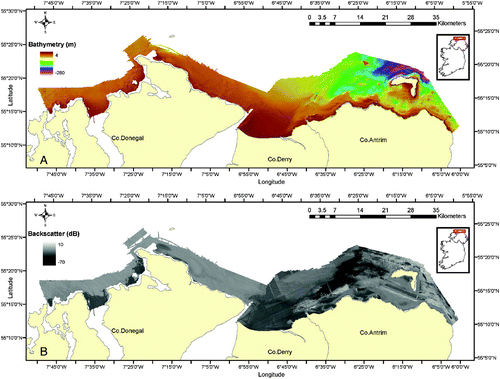
In 2007, a joint project was instigated by the UK Maritime and Coastguard Agency (MCA) and the Marine Institute of Ireland (MI) to survey the seabed within the 3 nautical mile strip between Fanad Head (Co. Donegal, Ireland) and Torr Head (Co. Antrim, Northern Ireland) using multibeam echo-sounder systems (MBES). This Joint Irish Bathymetric Survey (JIBS) programme was completed in September 2008 and resulted in an unprecedented high-resolution full seabed coverage bathymetric depth and backscatter intensity map of the north coast of Ireland (Figure 1). Although these data have been used for archaeological purposes (Plets et al., 2011; Westley et al., 2011), a lack of systematic ground-truthing information off the north coast of Ireland has meant that these data had not been used for geological or biological purposes.

Figure 1. Overview of (A) JIBS bathymetry data and (B) JIBS backscatter data off the north coast of Ireland.

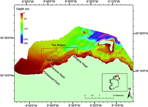
In 2010, the authors were commissioned by the Northern Ireland Environment Agency (NIEA) to derive a habitat map for a proposed Marine Scientific Area of Conservation (SAC) off the Causeway Coast, based on the data collected as part of the JIBS survey and the collation of diverse ground-truthing data acquired over the past 40 years by the British Geological Survey (BGS), NIEA, the Agri-Food and Biosciences Institute (AFBI), the University of Ulster (UU) and the National Museums Northern Ireland (NMNI). The proposed SAC is bounded by Ramore Head (Portstewart Point) to the west and Bengore/Benbane Head (Dunseverick) to the east with a northern limit just north of a submarine reef known as ‘the Ridges’ and the southern boundary defined by the coastline. This paper presents the seafloor substrate map resulting from this research, with as bounding coordinates: top left corner (6°43′36″W, 55°17′N) and top right corner (6°27′W, 55°17′N) (Figure 2).

Figure 2. JIBS multibeam bathymetry of the north coast of Ireland. Red box outlines the study area.

2. Methods

2.1. Ground-truthing data

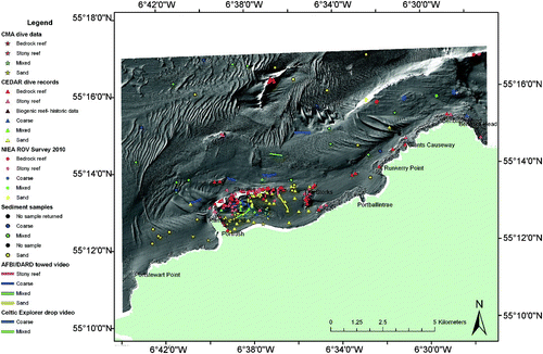
Ground-truthing data were gathered from a number of sources and included sediment samples, diver observations, towed underwater video surveys and remotely operated vehicle (ROV) surveys (Table 1). For each ground-truthing station, survey metadata, location, sediment data and interpreted substratum category were saved as an Excel spreadsheet before being converted into an ESRI shapefile for presentation and analysis in ArcGIS. Ground-truth stations were categorized into one of six classes: (1) bedrock reef; (2) stony reef, defined as any site with >10% cover of boulders or cobbles; (3) biogenic reef; (4) sand (ranging from very fine sand to very fine pebbles: 0.063–4 mm grain size); (5) mixed sediment (heterogeneous mixtures of gravel, sand and mud and often also shells and stones); and (6) coarse sediment (highly mobile cobbles and pebbles (shingle), together with gravel and coarse sand) (Figure 3). The classes are based upon the guidelines of the Marine Nature Conservation Review habitat classification scheme (Connor et al., 2004) and the modified Folk triangle (Long, 2006).

Table 1. Ground-truthing data available in the study area.

Year	Survey	Data type	Data provider
1973, 1978, 1979	BGS historic samples	Sediment samples	BGS
1988	Dredge disposal monitoring	Sediment samples	AFBI
1998	National Marine Monitoring Programme	Sediment samples	AFBI
2005	Portstewart Bay Waste Water Treatment Works Outfall Survey	Sediment samples	NIEA
2009	Hibernia optic cable survey	Sediment samples	UU
2009	UU's RV Celtic Explorer students cruise	Sediment samples	UU
1979, 1982–1985	Northern Ireland Sublittoral Survey	Diver surveys^a	NMNI
2006–2010	Sublittoral Survey of Northern Ireland	Diver surveys^a	NMNI
2006–2010	Seasearch	Diver surveys^a	NMNI
2004, 2010	Archaeological investigations	Diver surveys	UU
2000–2004	Northern Ireland Nearshore Subtidal Habitat Mapping Project	Underwater video	AFBI
2009	UU's RV Celtic Explorer students cruise	Underwater video	UU
2010	Skerries Marine SAC proposal	ROV survey	NIEA
^aCentre for Environmental Data and Recording database.

Figure 3. Overview of ground-truthing stations superimposed on bathymetry hillshade.

2.2. Multibeam data

The unprocessed raw (*.all files) data, containing the original depth soundings and backscatter values, and cleaned (xyz) (*.txt files) bathymetric data were supplied to the University of Ulster in 2009 by the MCA and MI for academic research. These cleaned data were subsequently imported into IVS Fledermaus DMagic software for gridding using a weighted moving average gridding algorithm (weight diameter 3) to a 1 m bin size and projected to UTM zone 29N. Fledermaus DMagic was used to create a Digital Elevation Model (DEM) from the resulting grid which was imported into IVS Fledermaus 7.0 for enhanced 3D visualisation and interpretation. In addition, the gridded data were exported as an ASCII grid for further analysis and interpretation in ESRI ArcGIS.

2.2.1. Bathymetric derivatives

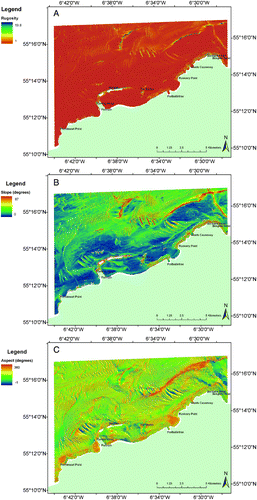
The cleaned bathymetric grid was subsequently used to derive a number of additional parameters. Firstly, within IVS Fledermaus rugosity was derived as a measure of terrain complexity (Figure 4A). Within ArcGIS, hillshading, bathymetric contour lines (20 m spacing), slope angle (in degrees, 0–90°; Figure 4B) and aspect (defined as the downslope direction in degrees, 0–360°; Figure 4C) were derived using the Spatial Analyst extension.

Figure 4. Parameters derived from the bathymetric data: (A) rugosity, (B) slope angle and (C) aspect.

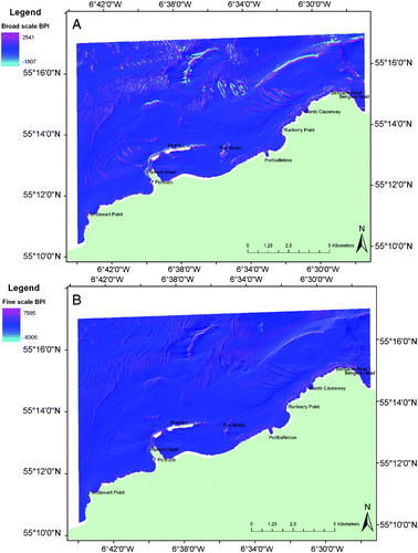
The Benthic Terrain Modeler extension for ArcGIS was used to calculate standardised fine- and broad-scale Bathymetric Position Indices (BPI) (Wright et al., 2005). BPI is a second-order derivative of a surface and may be defined as a measure of the elevation of locations with reference to the overall landscape (similar to the topographic position index used on land) (Verfaille, Doornenbal, Mitchell, White, & Van Lancker, 2007). When created, standardised, and examined at fine and broad scales, BPI provides a useful parameter for terrain classification (negative values indicate troughs and valleys; near zero values are typical for flat areas or areas with a constant slope; positive values represent highs and ridges). In this study, broad-scale BPI was calculated with an inner search radius of 10 m and an outer search radius of 100 m (scale factor of 100) (Figure 5A). The fine-scale BPI was calculated with an inner search radius of 1 m and an outer search radius of 20 m (scale factor of 20) (Figure 5B).

Figure 5. Parameters derived from the bathymetry using ArcGIS Benthic Terrain Modeler: (A) broad-scale BPI and (B) fine-scale BPI.

2.2.2. Backscatter

Until recently, multibeam data were predominantly used to create detailed bathymetric maps. However, some of the emitted acoustic energy, known as backscatter, reflects back to the sonar system and is mainly controlled by the hardness, the roughness and the morphological properties on the seabed. These data are conventionally presented as greyscale imagery showing the strength of the returning energy (backscatter), and once processed and stitched together are presented as a continuous image of the seabed reflectivity, called a mosaic. In the study area, multibeam data were acquired with two different systems (the Kongsberg EM3002 and EM710), each with their own specific properties and geometries, and deployed from two different vessels: RV Jetstream and RV Victor Hensen (Table 2). The processing and mosaicing of the raw data (*.all) were carried out for both datasets in IVS Fledermaus Geocoder, a software package designed to perform as many corrections (geometrical and physical) as possible to maximise the information content within the backscatter signal. The final mosaic was subsequently exported as ESRI ArcGIS ASCII files for further analysis.

Table 2. Overview of different vessels, multibeam systems and acquisition settings used in the study area as part of the JIBS project.

Vessel	Multibeam system	Sounding mode	Centre frequency (kHz)	Pulse length (μs)	File format
RV Jetstream	Kongsberg EM3002	1 (shallow)	293	149	.all
RV Victor Hensen	Kongsberg EM710	0 (very shallow)	71–97–83	206	.all
		1 (shallow)	71–83–77	500	.all

2.2.3. Automatic classification of the seafloor using QTC

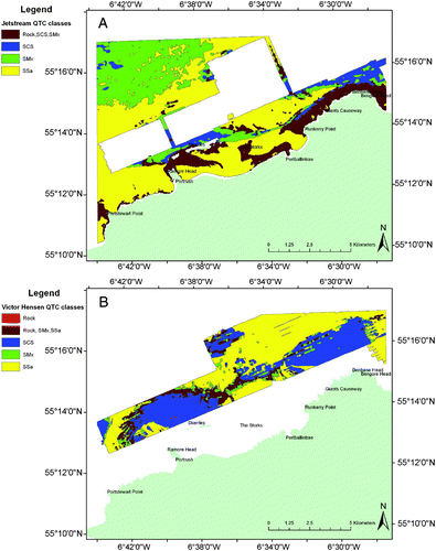
Quester Tangent Corporation's QTC Multiview software was used to build an unsupervised classification of the backscatter data using a technique called ‘segmentation’, the process of subdividing an image into homogenous regions or categories that correspond to different features, thus reducing complex information into a simplified, arbitrary representation. This was done primarily as an interpretive aid to identify boundaries between (or within) aggregations of similar units (in this case pixels). Owing to the fact that two different multibeam systems were used to collect the data, the backscatter data from each were processed separately, resulting in two classification maps (Figures 6 and 7). However, the same processing parameters were chosen for both datasets. The raw data were depth-cleaned using a threshold of 300 m and a rectangle dimension of 257 × 17 pixels was chosen, giving an average footprint of 13.7 m across track against 12.6 m along track; rectangles are the patches of the backscatter image from which features are generated (Quester Tangent Corporation, 2005, p. 157). These (full) feature vectors (FFVs) describe the variation in the backscatter imagery contained within each rectangular sample. The FFVs were reduced by Principal Components Analysis (PCA), in the manner described by Quester Tangent Corporation (2005, p. 157), to the three values most responsible for the variance in the dataset. The data were then subjected to a simulated k-means algorithm, which attempts to amalgamate the vectors into statistically logical groups (Preston, 2009), or classes. To speed up the process, 10% of all FFV samples were subjected to the auto-clustering process, using five iterations and running these in two batches (from three to 15 classes and from 16 to 30 classes). Finally, the data were divided into an optimum amount of classes (13 classes for the EM3002 system and 17 classes for the EM710 system) (Figure 6A, B). During processing, QTC was unable to compensate for the different frequencies used across the three sectors of the EM710. Autoclustering improved significantly after the beam was filtered between 5 and 50° despite the fact that this results in the loss of overlap between adjacent lines. In the next step, an interpolated map of the QTC classes was created using QTC CLAMS. The interpolation parameters were kept constant throughout each dataset and the final output grids were preserved at a 10 m cell size. The interpolation parameters were tested iteratively, before accepting a 100 m search radius base and a search size of 50 m. Finally, the classes were linked to the known ground-truthing data and reclassified in GIS to divide the interpolated map into four final classes: (1) rock (including both bedrock and stony reef), (2) mixed sediment (any sediment that has shelly material associated with it; SMx), (3) coarse sediment (>20% gravel; SCS) and (4) sand (SSa) (Figure 7A, B).

Figure 6. QTC classification map for (A) the EM3002 data acquired onboard RV Jetstream and (B) the EM710 data acquired onboard RV Victor Hensen.

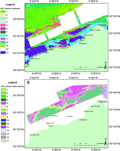
Figure 7. Reclassification of the QTC classes based on the available ground-truthing data for (A) the EM3002 data acquired onboard RV Jetstream and (B) the EM710 data acquired onboard RV Victor Hensen. SCS = coarse sediment; SMx = mixed sediment; SSa = sand.

2.2.4. Unsupervised classification using ArcGIS

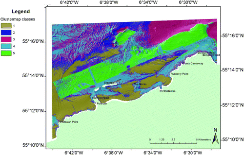
To aid further classification of the MBES datasets, unsupervised image-based classification was also undertaken within ArcGIS. The bathymetric-derived raster datasets were ‘stretched’ so pixel values fell on the 0–255 scale. The stretched rasters of broad BPI, slope angle, rescaled aspect (on to linear scale), rugosity, bathymetry and backscatter were subsequently combined into a composite raster (multi-band image), which was subjected to PCA to limit data redundancy and issues of high correlation between datasets. The resulting PCA-derived three-band raster image was analysed by the Isocluster (unsupervised classification) routine within ArcGIS to create a signature file for five classes (20 iterations, minimum class size of 20, sample interval of 10). Finally, maximum likelihood classification was used on the PCA multi-band image using the signature file to classify the data (Figure 8). A pronounced linear artefact can be seen in the resulting clustermap which is due to the differences in the input backscatter mosaics caused by the fact that data were acquired using two different multibeam systems.

Figure 8. ArcGIS clustermap resulting from PCA and unsupervised classification of broad BPI, slope angle, aspect, rugosity, bathymetry and backscatter.

3. Resulting classes

A final substratum map was drawn in ArcGIS combining all data discussed above. The QTC classification was the primary driver, while the other individual datasets as well as the clustermap were used to refine boundaries and support the QTC classification. In total, 10 different classes were recognised Main Map).

3.1. Bedrock reef

Bedrock reef was identified from the QTC classification but the final boundary was drawn using a visual interpretation of the hillshade (derived from the bathymetric data), clustermap and ground-truthing data to distinguish this class from stony reef.

3.2. Stony reef

Stony reef is defined as stable boulders and cobbles, with less than 10% of exposed bedrock. A relatively low spread of ground-truthing points exists for this substratum (the highest concentration is around the Skerries) and a distinction between bedrock and stony reef was made visually using the textural patterns in the bathymetric data. In areas where stony reef is next to sediment (particularly sand) the boundary is much clearer and defined clearly by QTC.

3.3. Scoured bedrock with veneer of mobile sediment

The largest area of this substratum is to the north of Benbane Head (Main Map). Although QTC classified this entire platform as coarse sediment, the backscatter image clearly shows areas dominated by very high backscatter and low backscatter E–W ‘streaks’ (representing softer smoother material). One of the ROV stations described the seabed as sand over bedrock, whilst all other (three) ROV stations suggest a mixed coarse sediment cover. Other areas/features classified as scoured seabed with a veneer of mobile sediment had no ground-truthing points, but QTC classified these as rock whereas the bathymetry and backscatter data suggest some presence of sediments.

3.4. Coarse sediment

Coarse sediment areas were picked out partially by QTC, especially the larger zones. However, the final boundaries were drawn manually, guided by QTC, but predominantly using the backscatter image as the coarser sediments correspond to areas of higher backscatter (lighter coloured). Only a single ground-truthing point (grab sample) was available and is described as fine-to-medium sand with coarser sand and shell fragments. However, as this sample point is very close to the boundary with the mixed sediment, it might not be truly representative of this facies.

3.5. Coarse sediment with some shelly material

While QTC classified this facies as coarse sediment (which is also confirmed by three video-tows), the majority of the sediment samples taken suggest gravelly sand with shelly material; hence this separate class of coarse sediment but with some shell.

3.6. Mixed sediment

A mixture of sand and small amounts of gravel (<20%) and shelly material corresponds to areas with a distinct higher backscatter than the surrounding seabed. Just to the south of the Skerries, QTC was not able to differentiate the mixed sediment facies from the adjacent bedrock and stony reef region but did pick out a clear boundary between this facies and the surrounding softer seabed sediments (darker areas on the backscatter image). A reclassification was therefore performed, based on the ground-truthing information and backscatter image, but guided by the QTC boundary. In other areas where mixed sediment was identified by QTC, the boundaries as defined by QTC were re-drawn manually based on the backscatter image.

3.7. Mobile sand over mixed sediment

On the backscatter image, this area is characterised by darker streaks (interpreted as sand) on top of a lighter coloured (i.e. higher backscatter) seafloor, interpreted as mixed sediment.

3.8. Fine and medium sand

This is the most extensively occurring substratum in the study area. The sandy sediment, and its boundary with different types of substratum, was identified well by QTC, which even distinguished smaller patches of sand on the basaltic rock platforms. From the backscatter image, the sandy sediment is represented by the darkest colours (low backscatter) and often shows a sharp clear boundary where it occurs next to coarser sediments. Fifty-nine ground-truthing stations within the sand polygons confirm the interpretation of this substratum. In general, the inshore sand facies appears to be mobile fine sand, as shown by ground-truthing, while the offshore sand appears to be mobile medium-fine-grained sand with occasional shell fragments.

3.9. Coarse sand

The bank to the north-west of the Skerries is interpreted as comprising coarse sand. The QTC results of the data acquired with the Kongsberg EM710 indicate a sandy substratum, as do the presence of large sediment waves and a single dive survey sample. However, on the backscatter image, this sand bank appears lighter than the sandy areas in the vicinity (i.e. higher backscatter). This, together with a video-tow indicating coarse sediment over the sand bank has led to the interpretation that the bank is possibly made up of coarser sand.

3.10. Possibly sand

This area is located to the north and east of the large plateau to the north of Benbane Head. It appears on the backscatter image as relatively dark (i.e. low backscatter) and is classified as sand by the QTC process. However, there are only two ROV ground-truthing stations on the edge of this facies, no distinct bedforms are developed within it and the backscatter tone is lighter than the sandy area interpreted to the northwest – this could either mean that the sand is slightly coarser than the adjacent seafloor or that this represents a thinner sand layer over a harder substratum.

4. Discussion and conclusion

The Main Map is the first substratum map for the north coast of Northern Ireland based on the integration of high-resolution, full seabed coverage swath bathymetry and backscatter data, and 40 years of ground-truthing data. It shows a dominance of sandy (fine to medium) sediments with most of the exposed bedrock and stony reef closest to shore. In some areas, broken shells make up an important part of the sediment composition.

However, as evidenced from the ground-truthing maps, ground-truthing stations are mainly concentrated around the Skerries Islands and some of the identified facies have very few ground-truthing stations associated with them (Table 3).

Table 3. Surface area for each acoustic class, number of ground-truthing stations and number of ground-truthing stations supporting the interpretation.

Class	Area (km^2)	No. of ground-truthing stations	No. of ground-truthing stations in agreement	Notes
Bedrock reef	4.9	54	44	Majority of samples not in agreement were classified as stony reef
Stony reef	4.9	49	27	Majority of samples not in agreement were classified as bedrock reef
Scoured bedrock with veneer of mobile sediment	13	7	1	One video-tow confirms this interpretation; other samples indicate bedrock reef or coarse sediment
Coarse sediment	3.4	1	0	Sample classified as sand but has some (<10%) gravel-sized material
Coarse sediment with some shell	12	13	12
Mixed sediment	22.8	52	18	More recent data confirm mixed sediment, older data suggest stony reef and sand with relatively small amount of dead shells
Mobile sand over mixed sediment	0.16	3	1	Confirmed by one dive, other samples indicate stony reef and mixed sediment but give no indication on mobility of the surface sediments
Fine and medium sand	62.7	71	59
Coarse sand	2.3	2	0	One sample described as sand, one sample described as coarse sediment (>20% gravel)
Possibly sand	5.1	2	1	Sample not in agreement suggests stony reef

Furthermore, the north coast of Ireland is very exposed and under constant influence of the waves and swell of the North Atlantic. The tidal streams generally flow west to east, resulting in an eastward movement of offshore sediment. Closer to shore, eddies form in the bays and rip currents occur near rocks at the end of the bays (Carter, 1991). Tidal banks and sand waves observed on the bathymetry data suggest a complicated flow pattern and active sediment transport. This, combined with the fact that the ground-truthing records date back several years to several decades, and the occurrence of very mobile substrate in places, make it very likely that the seabed has changed in the time period between the sampling surveys and the acquisition of the multibeam data.

A further issue regarding the reliance on extant ground-truthing datasets is that of scale: over many facies the ground-truthing datasets available could not capture the sediment type or variability at a resolution appropriate to the minimum mappable unit (1 m²) from the multibeam data.

Nevertheless, although the accuracy and confidence level for some of the acoustic facies may be low, the Main Map is the most accurate to date and can be used for biological, geological and hydrodynamic studies as well as a base map for planning more systematic ground-truthing surveys in areas where such data are clearly missing.

Acknowledgements

This project was conducted for, and financed by, NIEA. The authors wish to thank Julia Nunn of NMNI for her assistance in accessing the CEDaR dive records, Claire Goodwin of NMNI for provision of dive photographic images and personal observations, Charmaine Beer (Seasearch Northern Ireland) for provision of Seasearch dive forms, Matthew Service of AFBI for providing background literature and dredge disposal monitoring historic datasets, Tim Mackie of NIEA Water Management Unit for providing the Portstewart Waste Water Treatment Works grab sample data, Dave Long of BGS for assistance with locating historic sample data and provision of digital resources, Kieran Westley of the Centre for Maritime Archaeology (University of Ulster) for provision of archaeological dive data and Gail McAleese for processing some of the grab samples. Vibrocore data off Portrush were collected as part of the Hibernia Project, courtesy of METOC PLC. Finally, thanks to Dr Riccomini, Dr Lo Iacono and Dr Blondel for their reviews which helped to improve this paper.

Software

Data gridding of the multibeam bathymetry was performed using IVS Fledermaus DMagic 7.0, while the backscatter data was mosaiced using IVS Fledermaus Geocoder 7.0. The automatic segmentation was carried out in QTC Multiview 4.0 and this unsupervised classification was interpolated in QTC Clams 4.0. All data were brought together in ESRI ArcGIS 9.2 for further analysis and final map creation.

References

- Carter , B. 1991 . Shifting sands: A study of the coast of Northern Ireland from Magilligan to Larne Countryside and Wildlife Research Series. HMSO: Belfast
- Connor , D. W. , Allen , J. H. , Golding , N. , Howell , K. L. , Lieberknecht , L. M. , Northen , K. O. and Reker , J. B. 2004 . The marine habitat classification for Britain and Ireland (version 04.05) [Internet version] , Peterborough , , UK : JNCC . Retrieved October 22, 2008, from http://www.jncc.gov.uk/MarineHabitatClassification
- Long , D. 2006 . BGS detailed explanation of seabed sediment modified Folk classification Retrieved June 24, 2010, from http://www.searchmesh.net/PDF/GMHM3_Detailed_explanation_of_seabed_sediment_classification.pdf
- Plets , R. , Quinn , R. , Forsythe , W. , Westley , K. , Bell , T. , Benetti , S. , McGrath , F. and Robinson , R. 2011 . Using multibeam echo-sounder data to identify shipwreck sites: Archaeological assessment of the Joint Irish Bathymetric Survey data . International Journal of Nautical Archaeology , 40 ( 1 ) : 87 – 98 . DOI: 10.1111/j.1095-9270.2010.00271.x
- Preston , J. 2009 . Automated acoustic seabed classification of multibeam images of Stanton Banks . Applied Acoustics , 70 : 1277 – 1287 . DOI: 10.1016/j.apacoust.2008.07.011
- Quester Tangent Corporation . 2005 . QTC multiview acoustic seabed classification for multibeam sonar, user manual and reference (version 3.0) Quester Tangent Corporation: Sidney, B.C., Canada
- Verfaillie , E. , Doornenbal , P. , Mitchell , A. J. , White , J. and Van Lancker , V. 2007 . The bathymetric position index (BPI) as a support tool for habitat mapping Retrieved November 20, 2011, from http://www.searchmesh.net/pdf/GMHM4_Bathymetric_position_index_(BPI)pdf.
- Westley , K. , Quinn , R. , Forsythe , W. , Plets , R. , Bell , T. , Benetti , S., McGrath, F. and Robinson , R. 2011 . Mapping submerged landscapes using multibeam bathymetric data: A case study from the north coast of Ireland . International Journal of Nautical Archaeology , 40 ( 1 ) : 99 – 112 . DOI: 10.1111/j.1095-9270.2010.00272.x
- Wright , D. J. , Lundblad , E. R. , Larkin , E. M. , Rinehart , R. W. , Murphy , J. , Cary-Kothera , L. and Draganov , K. 2005 . ArcGIS Benthic Terrain Modeler , Corvallis , OR : Oregon State University, Davey Jones Locker Seafloor Mapping/Marine GIS Laboratory and NOAA Coastal Services Center . Retrieved February 10, 2012, from http://www.csc.noaa.gov/digitalcoast/tools/btm/index.html