High-resolution geomorphological map of a low mountain range near Aachen, Germany

Abstract

A high-resolution geomorphological map covering the central part of a low mountain range close to the city of Aachen in the border region of western Germany and eastern Belgium is presented. It is conceptually based on the ‘Geomorphologische Karte 1:25,000’ (GMK) which was developed by German researchers in the 1970s and 1980s but differs from the original concept in terms of data acquisition, processing and map layout in order to overcome some problems of classical geomorphological maps. These comprise time consuming field work, inflexible paper-based map creation, and the resulting poor legibility due to extremely high information density. All mapping was performed in a Geographic Information Systems (GIS) environment on the basis of a 1 m LiDAR digital elevation model to reduce the time and cost needed for map production. The scale of the map is 1:5000 and thus increased by a factor of five in comparison to the original GMK to make sure no crucial information is lost through cartographic generalization. The layout was adjusted to fit the larger scale, resulting in an improvement of the morphometric information value and a strengthening of the GMK's construction kit concept. In comparison to the original GMK concept, the methodology yields benefits for the production of geomorphological maps by reducing the effort necessary to collect and manage data, improving the spatial accuracy, and enhancing the flexibility regarding data management and map layout.

Keywords:

• Geomorphological map
• GIS
• remote sensing
• LiDAR
• high-resolution DEM
• scale 1:5000

1. Introduction

Geomorphological maps can be of great value not only for geomorphologists but also for many neighboring fields of science (e.g. soil science and biology) and for numerous practical applications that depend on precise geomorphological data, such as natural hazard assessments, environmental planning, and construction engineering (Finke, 1980; Kienholz, 1980; Paron & Claessens, 2011). A noticeable reactivation of the subject can be observed in geomorphological publications over the recent years (e.g. Gustavsson, Kolstrup, & Seijmonsbergen, 2006; Smith, Paron, & Griffiths, 2011). However, in most cases makers and users of geomorphological maps are both geomorphologists with the exception of several highly specialized industries directly dependent on geomorphological data like those mentioned before. The latter tend to be interested in querying certain information rather than interpreting complex maps (Paron & Claessens, 2011).

This lack of popularity is primarily caused by two facts: first, depicting the three dimensional features of the Earth's surface with all its relevant attributes – morphometry, morphodynamics, morphochronology, morphostructure and morphogenesis – in a single map is a requirement, which is hard to fulfill. This problem has been subject to several large scientific research projects which are briefly reviewed in Otto, Gustavsson, and Geilhausen (2011). These comprise the IGU's concept as an international approach (Bashenina, Gellert, Klimaschewski, & Scholz, 1968; Demek, 1972) and further several large national conceptions out of which the German ‘Geomorphologische Karte 1:25,000’ (GMK, Göbel, Leser, Stäblein, & Werner, 1975) is one of the most sophisticated approaches. Its outstanding advantage is the construction kit concept, by which the combination of several layers of information sums up to the definition of the geomorphological environment (Barsch & Liedtke, 1980; Barsch & Mäusbacher, 1979). It was promoted by a priority research program in which eight sheets at a scale of 1:100,000 and 27 sheets at a scale of 1:25,000 were completed (available at: http://gidimap.giub.uni-bonn.de/gmk.digital/home_en.htm). Nevertheless, geomorphological maps still tend to contain an extremely high information density which in turn often causes poor legibility. However, as many aspects of the problem are intrinsic to printed maps the techniques offered by modern Geographic Information Systems (GIS) may provide useful starting points here.

Second, the classical field work-based creation of geomorphological maps is very time-consuming and therefore cost-intensive (Barsch & Mäusbacher, 1982). This hampering factor originates from the manpower needed to map and describe the features precisely in the field. A new generation of digital elevation models (DEM) with resolutions of 10 m and below may provide the key to map even small geomorphological features quickly and precisely using modern remote sensing and GIS techniques.

The map presented here (see Main Map) is the result of a study which aimed to determine to what extent expert-driven manual interpretative geomorphological mapping from a high-resolution DEM in a GIS environment may overcome the classical problems described above. This was performed by evaluating if it is feasible to extract the layers of information given in the GMK concept from 1 m LiDAR-DEM. These eight layers comprise: topography, slope angle, landforms (steps, closed hollow forms and closed full forms, surface roughness, and valleys), curvature, substrate, process, hydrography, and areas of geomorphic structures and processes (Barsch & Liedtke, 1980). Earlier studies such as Smith, Rose, and Booth (2006), Jones, Brewer, Johnstone, and Macklin (2007), and Lehmkuhl, Loibl, and Borchardt (2010) showed that mapping morphography from DEM data is generally possible. The approach behind this map goes further and is aiming toward a complete high-resolution survey of geomorphology from state-of-the-art DEM data.

2. Study area

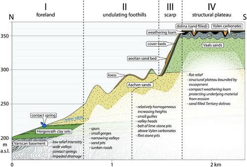
The study area is located south of the city of Aachen, Germany, in a hilly area called ‘Aachener Wald’ (engl.: ‘Aachen forest’). The German-Belgian border runs through the southern part of the map. Local geology is dominated by a series of marine sediments of late Cretaceous and early Tertiary age with a total thickness of about 200 m. These sediments were deposited upon a former peneplain of the Variscan basement (Knapp, 1980a; Richter, 1985). A relatively thin layer of clay at the base of the Cretaceous sequence is overlain by several much thicker sand layers. At the top, distinct karstic features, typically flat dolines of about 5 m in diameter have developed in the dominating limestone. A layer of about 2–5-m thickness consisting of compact loam covering the limestone is the product of intense Tertiary weathering of carbonates. This layer and the limestone protect the underlying uncemented sediments from the rapid erosion that is evident in all areas where these two layers are absent (Ribbert, 1992). During the Pleistocene, loess was locally accumulated and reworked by periglacial slope processes into solifluidal cover-beds in most cases (Figure 1, Lehmkuhl, 2011).

Figure 1. Simplified cross section of the northern part of study area from the foreland toward the plateau (7× vertical exaggeration).

The regional climate is controlled by the geostrophic position within the extratropical prevailing westerlies. Aachen is usually located south of the frontal zone between the Azores high and Iceland low-pressure systems and local weather is thus dominated by passing low-pressure cells, resulting in unstable weather (Havlik, 2002). Annual average temperature is +10.1°C and the average annual rainfall is 801 mm in the period 1971–2000 (Mühr, 2007). Of particular relevance for present day geomorphological processes is the torrential rainfall during thunderstorms in summer with rainfall of ∼60 mm in several hours (Havlik, 2002). The potential natural vegetation for the region is an impoverished woodrush beech or beech oak forest (Pflug et al., 1978).

The landforms in the area show the strong influence of both geology and climatic change through geological time. The latter has resulted in an interplay of subtropical weathering in the Tertiary, periglacial slope processes in Quaternary glacial periods and fluvial erosion in Quaternary interglacial periods including the Holocene (Lehmkuhl, 2011). Based on the analysis of absolute elevations, four geomorphological units on mesorelief scale can be quantified (Figure 1). (I) The lowest areas show low relief intensity and are dominated by wide valleys. On the map, this unit is characterized by green and brown colors, indicating that fluvial and denudational processes were primarily shaping the surface. (II) In the next higher unit, spurs and narrowing valleys are the most prominent features of the mesorelief. In many cases, hummocky terrain can be found on top of the spurs. (III) Going further up the slopes, a zone of relatively homogeneous increase in height follows, into which only few valley heads penetrate. On the map, units II and III are recognizable by pink lines in the color fills. These show an additional cryogenic influence in the denudational areas, delineating the solifluidal cover-beds. Unit III can best be distinguished from unit II by steeper slopes. (IV) The highest unit reflects nearly flat areas on top of the range which are forming a structural plateau. These are the areas where weathering loam resides above Cretaceous limestone. They can be easily identified by the light blue color that is used for karstic features following the GMK legend. Remarkably, similar geomorphological units can be found on both sides of the main ridge but all units are located higher on the southern side. For example, the southern lowlands reach down to about 200 m a.s.l., while the northern lowlands do not extend below 240 m a.s.l., although the horizontal distances to the highest elevations in the study area are similar. This emphasizes the dependency of the geomorphological units on the local relief and geological substrates. The former is strongly influenced by different levels of the receiving streams to the north and south and the latter by the slight tilting of the layers (Figure 1).

As the city center of Aachen is only 5 km north of the study area, human influence on the landscape was strong since several thousand years. The earliest evidence of human activity in the vicinity of Aachen (e.g. mining of flintstone) dates back to the late Paleolithic (Kunow & Wegner, 2006; Schyle, 2011). Later a relatively large number of sand pits and limestone or marl pits were established. Numerous sunken roads toward these pits and sunken roads close to the main historic trade road from Aachen to Liège to Brussels show the human impact on the landscape from Roman-to-modern times, particularly in the areas where Cretaceous sands are outcropping. An additional focus of the prehistoric and ancient valuation of natural resources was lumber, resulting in a scrub dominated vegetation cover that lasted until an enactment of the local government, which assigned the primary function of a local recreation area to the Aachen forest in 1882 (Kaemmerer, 1967). Today, human impact on the area is predominantly caused by transportation (e.g. a major trunk road and railway tunnel) between the regional centers of Aachen/Cologne and Liege (Meyer, 1989). Furthermore, large parts of the area are allocated as local recreation zones resulting in an extensive network of pedestrian walkways (Poll, 2003). The vegetation cover has changed to beech dominated high forest intersected by large patches of spruce and pine plantings (Forstamt Aachen, 1982).

3. Methods

A LiDAR-DEM of 1-m resolution provided by North Rhine-Westphalia's State Surveying Authority served as base mapping. This DEM is a last echo product in which buildings and vegetation have been removed automatically to provide an approximation of the bare earth surface (Bezirksregierung Köln, 2011a). Additionally to the DEM, only data that was available freely or at low cost was used in order to assure that the mapping methods can be applied to other study areas as well. This data comprised Google Earth and Landsat ETM+ imagery for initial surveys, a geological map at a scale of 1:100,000 (Knapp, 1980b) to evaluate the influence of substrate on the landforms, and topographical maps (see below).

In order to assess the quality of the DEM and of the derived landform mapping about half of the study area was field surveyed for ground truthing purposes. This included precise measurements of more than 100 landforms by GPS (averaged waypoints with a Garmin 60CSX device), mirror compass and measuring tape. The landforms were then mapped on the basis of the topographic map with the highest resolution publically available in Germany, the ‘Deutsche Grundkarte 1:5000’ (DGK5, engl.: ‘German Base Map 1:5000’) provided by North Rhine-Westphalia's State Surveying Authority (Bezirksregierung Köln, 2011b). Measurement techniques of higher accuracy, e.g. leveling, were too time-consuming to be used efficiently in extensive surveys. To evaluate the accuracy and spatial quality of field work and DEM-based mapping, we examined how the field results (Figure 2) and the German Base Map (Figure 3) fit the LiDAR data in the GIS environment.

Figure 2. Averaged GPS waypoints taken at the centers of landforms during field work in the forest: (a) GPS waypoint with random offset from the position in the DEM, (b) GPS waypoints fit the DEM, (c) landforms not detected in the field due to dense vegetation cover.

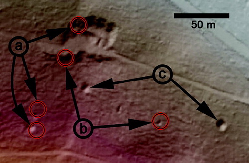
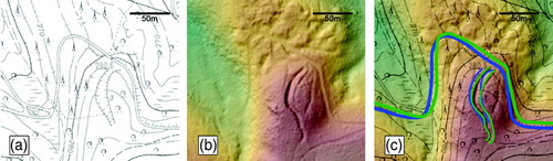
Figure 3. Detail from (a) the German Base Map 1:5000 and (b) the DEM. The overlay in (c) shows the edges of a sunken road and a pedestrian walkway marked in green (DEM) and blue (map). The offsets are up to ca. 10 m here. The distribution of offsets is random over the whole study area and can therefore not be corrected.

In a first step, hillshade, aspect, slope, and curvature were processed from the DEM. Both horizontal and vertical curvature were then classified and combined to generate a raster of landform elements. Morphological interpretation of these information layers formed the basis for the delineation and morphometric parameterization of all landforms in the map. The slope raster was classified, converted into polygons and generalized to produce a slope layer of information similar to the GMK legend.

Due to the German-Belgian border running through the study area, a topographic map with a level of detail high enough to locate and depict microscale features covering the whole study area was not available. Thus, contour lines (2.5, 5 and 10 m) were generated from the DEM and subsequently smoothed. The major topographic features (buildings, roads, etc.) were mapped manually from remotely sensed imagery. These and the contours were then used as a topographic base layer for the geomorphological map. Curvature lines showing linear maxima in convexity and concavity were mapped manually using the contour lines and the curvature raster with an overlay of the hillshade at 50% transparency.

In order to retain the classifications and differentiations postulated in the GMK concept in the GIS environment, the landforms had to be split into six individual layers: thalwegs, linear hollow landforms, linear full landforms, closed hollow landforms, closed full landforms, and steps. The landforms were then derived by expert-driven manual interpretative mapping from the DEM and the derivates described above. Satellite imagery was only used to support DEM interpretation, not as base layer for mapping. The interpretation of this information was, however, hampered by low image resolution and dense vegetation in many cases. Morphogenetic and morphographic information was attributed to each landform mapped by assigning it to a landform element in a database of landforms (see 13 Abbreviations in the legend). The morphometric differentiation is based on manual measurements from the DEM and subsequent classification. For several landforms, it was not possible to determine the primary forming processes. In these cases the morphogenetic information was gathered in the field after completion of the GIS mapping. In the map, this is indicated by a ‘*’ added to the abbreviation.

Mapping hydrological features required a set of different techniques. The stream lines were first processed from a hole-filled version of the DEM using the flow direction, water accumulation and stream definition tools and then corrected manually in order to remove errors that were introduced by features crossing the thalwegs, such as bridges or dams. Lakes were extracted semi-automatically by selecting areas bigger than 25 m² where slope values are smaller than 0.01° from the DEM and subsequent evaluation of the results with aerial photographs. Even though the local geology and its hydrological implications could be approximated from the geological map, the precise determination of source locations remained subject to a high level of uncertainty. Detection of waterlogged and seepage areas was not possible from the DEM and aerial photographs.

The ‘areas of geomorphic structures and processes’ layer is intended to show the structures and processes that are ‘responsible for the latest significant shaping of the respective part of relief’ (Barsch & Liedtke, 1980). They were mapped manually from the digital data by interpretation of the morphographic situation. This was performed in a descending order of certainty with which areas can be attributed to a specific process primarily shaping it.

Substrates and processes were not integrated into the map for different reasons. For the substrate layer, the initial idea to combine the information on local geology derived from the geological map with that of the topography to map morphostructure had to be rejected. As the available remote sensing data give no robust clues on the subsurface situation, the generated spatial data would have been largely hypothetical and clear delineations impossible. Regarding the processes layer, the high level of detail at the 1:5000 target scale resulted in a situation, where all processes that were detectable from the data were resulting in landforms that could be directly mapped. Thus, the information content of the processes layer was widely redundant with the landforms layer due to the inability to gather information on processes on scales below the DEM resolution. Therefore, a separate layer for processes was obsolete. However, these are specific results of the remote sensing and DEM-based mapping method which indicate that these layers of information can only be acquired by field work.

4. Map design

As the aim of the study was to evaluate whether it is possible to extract the GMK's layers of information from the DEM, the layout mostly adheres to the principles given there (Barsch & Liedtke, 1980; Göbel, Leser, Stäblein, & Werner, 1975). The reference system is the German national grid ‘Gauß-Krüger’, a transverse Mercator projection similar to UTM but with central meridians situated at each 3° step and the Bessel ellipsoid which is optimized for central Europe. The bold printed last three digits of the coordinates represent hundred meters. Differing from the GMK concept, instead of 1:25,000 a scale of 1:5000 was chosen to make sure that less information is lost through generalization (Leser 1980). This is attended by an increase of importance of singular and minor landforms which are supposed to be depicted by a vast set of symbols differentiated by genesis in the original concept. Due to the high resolution it was possible to display even the smallest relevant landforms by a set of morphometrically classified saw-toothed line symbols which were originally allotted to steps (see legend elements 1, 2, and 3). This strengthens the quantitative informative value and the construction kit concept. In order to retain a high level of morphogenetic substance, morphogenetic abbreviations that were used as annotations to the landforms were introduced (see legend element 13).

Due to the GMK Base Map's focus on morphogenesis, the color fills are reserved to the ‘areas of geomorphic structures and processes’ layer in order to emphasize its relevance. The color palettes and systematics were adopted. Classified slope angles are displayed by different hachures of thin black lines. Differing from the GMK concept, the classification steps of the slope layer were adjusted to increase systematically (0.5°, 1°, 2°, 4°, etc.) to improve cartographic quality and legibility. Curvature is implemented by gray lines depicting the apexes of prominent concave (dashed) or convex (continuous) features and point signatures for singular hillocks and depressions. The GMK legend's distinction between different curvature radiuses was omitted due to the questionable scientific concept behind it (Spönemann & Lehmeier, 1989). The only features that still had to be depicted by morphographical signatures were the small drainageways and other small linear features, because their diameter often falls below the critical representable limit of about 5 m equaling 1 mm in the map at the scale of 1:5000. Symbolization of the roughness of aerial relief elements and hydrography follows the GMK concepts.

As all layers of information are stored in separate GIS layers any other layer combination and layout for applied maps is possible.

5. Conclusions

If feasible efforts of time and equipment are assumed, the comparison of field mapping and mapping from a high-resolution DEM in a GIS environment indicates that the accuracy attainable from the LiDAR DEM is higher than that of traditional field work. Furthermore, the LiDAR-DEM's reproduction of topography proved to be more precise than that of the German base map at 1:5000.

The map shows that the production of large-scale geomorphological maps from high-resolution DEM data is possible, even in settings of high landform density and complexity. The general optical impression is close to that of the original GMK, even though some layers of information had to be excluded (e.g. processes, substrates) and others were changed conceptually for different reasons (e.g. landforms, slope angles).

Evaluating the results, some distinct differences to the fieldwork-derived GMKs can be accounted for. The morphometric information value was strongly enhanced as a consequence of the larger scale which allows the display of all landforms (except the small linear ones) by symbols differentiating by height/depth and width. This improves the construction kit concept as well, because many features that required unique morphographic signatures can now be depicted by a combination of their precise and morphometrically quantifiable outlines using other layers of information. From a technical perspective, the methodology based on remote sensing and spatial analysis results in a reduction of time and costs needed to gather geomorphological data. The GIS environment provides more flexibility in terms of organization and presentation of the data and enables the researcher both to use any selection of layers and to combine it with other data (e.g. geological maps or soil maps) depending on the specific research questions. The work flow offers the opportunity to map geomorphology quickly at high levels of detail and then validate, refine, and complement the data by concerted field work. Whether these conceptual and practical advantages can outweigh the drawbacks caused by the exclusion of processes and substrates or the uncertainties (e.g. in the hydrology layer) will probably be dependent on study areas and research focuses.

As the layout sticks closely to that of the GMK, many advantages, such as the high level of flexibility and distinctness, as well as drawbacks, such as too high complexity reducing map legibility, are passed on from the GMK to the map presented here. Yet, the GIS environment decouples data and design and thus enables the geomorphologist to fit the map layout to each study's topic and thus rapidly produce applied geomorphological maps. From this perspective the unifying map legends are valuable concepts which might be used as guidance in geomorphological map production but each of them are far too inflexible to be used exclusively. Furthermore, the GIS environment supports the query-driven handling of geomorphological information that is favored by private companies and therefore strongly increases the scientific benefits and potential value of the mapping efforts.

6. Software

To ensure a high level of reproducibility of the techniques and results all data processing, mapping and map design was performed in ESRI ArcGIS 9.3. Additionally, Adobe Illustrator CS4 was used for specific vector file optimizations for the final PDF-file export.

Acknowledgements

We thank Georg Stauch for scientific input that essentially helped in developing the concept and creating the map. The reviewers, the Editor, and our colleagues Hendrik Merbitz and Veit Nottebaum are thanked for many valuable comments that helped to improve the map and strengthen the manuscript.

References

- Barsch , D. and Liedtke , H. 1980 . Principles, scientific value and practical applicability of the geomorphological map of the Federal Republic of Germany at the scale of 1:25000 (GMK 25) and 1:100000 (GMK 100) . Zeitschrift für Geomorphologie Supplement , 36 : 296 – 313 .
- Barsch , D. and Mäusbacher , R. 1979 . Geomorphological and ecological mapping . GeoJournal , 3 ( 4 ) : 361 – 370 . doi: 10.1007/BF00221238
- Barsch , D. and Mäusbacher , R. 1982 . “ Erfahrungen und Entscheidungen der Koordinationskommission ” . In Beiträge zum GMK-Schwerpunktprogramm III – Erträge und Fortschritte der geomorphologischen Detailkartierung Edited by: Barsch , D. and Stäblein , G. 27 – 30 . Freie Universität Berlin, Berlin
- Bashenina , N. V. , Gellert , J. F. , Klimaschewski , M. and Scholz , E. 1968 . Project of the unified key to the detailed geomorphological map of the world, Polska Akademie Nauk, Folia geographica . Ser Geogr Phys , 3 ( 2 ) : 1 – 40 .
- Bezirksregierung Köln (2011a). Digitale Geländemodelle (DGM), URL Retrieved from: http://www.bezreg-koeln.nrw.de/brk_internet/organisation/abteilung07_produkte/reliefinformationen/gelaendemodelle/index.html.
- Bezirksregierung Köln (2011b). Deutsche Grundkarte 1:5.000 (DGK5), URL Retrieved from: http://www.bezreg-koeln.nrw.de/brk_internet/organisation/abteilung07_produkte/topographisch/dgk5/index.html.
- Demek, J. (1972). Manual of detailed geomorphological mapping, Prague.
- Finke , L. 1980 . “ Anforderungen aus der Planungspraxis an ein geomorphologisches Kartenwerk ” . In Methoden und Anwendbarkeit geomorphologischer Detailkarten Edited by: Barsch , D. and Liedtke , H. 75 – 81 . Freie Universität Berlin, Berlin
- Forstamt Aachen (1982). Jahrhundertweg – ein Spaziergang durch „100 Jahre Aachener Erholungswald“, Aachen.
- Göbel , P. , Leser , H. , Stäblein , G. and Werner , R. 1975 . Geomorphologische Kartierung – Richtlinien zur Herstellung geomorphologischer Karten 1:25.000 1 – 33 . Freie Universität Berlin, Berlin
- Gustavsson , M. , Kolstrup , E. and Seijmonsbergen , A. C. 2006 . A new symbol-and-GIS based detailed geomorphological mapping system: Renewal of a scientific discipline for understanding landscape development . Geomorphology , 77 ( 1–2 ) : 90 – 111 . doi: 10.1016/j.geomorph.2006.01.026
- Havlik, D. (2002). Das Klima von Aachen, Aachener Geographische Arbeiten Aachen, 1–20.
- Jones , A. F. , Brewer , P. A. , Johnstone , E. and Macklin , M. G. 2007 . High-resolution interpretative geomorphological mapping of river valley environments using airborne LiDAR data . Earth Surface Processes and Landforms , 32 ( 10 ) : 1574 – 1592 . doi: 10.1002/esp.1505
- Kaemmerer, W. (1967). Geschichtliches Aachen – Vom Werden Und Wesen Einer Reichsstadt, Aachen.
- Kienholz , H. 1980 . “ Beurteilung und Kartierung von Naturgefahren ” . In Methoden und Anwendbarkeit geomorphologischer Detailkarten Edited by: Barsch , D. and Liedtke , H. 83 – 90 . Freie Universität Berlin, Berlin
- Knapp, G. (1980a). Geologische Karte der nördlichen Eifel 1:100.000, Krefeld.
- Knapp, G. (1980b). Erläuterungen zur Geologischen Karte der nördlichen Eifel 1:100.000, Krefeld.
- Kunow, J., & Wegner, H. H. (2006). Urgeschichte im Rheinland, Verl. des Rheinischen Vereins für Denkmalpflege und Landschaftsschutz, Köln.
- Lehmkuhl , F. 2011 . “ Die Entstehung des heutigen Naturraums und seine Nutzung ” . In Aachen – von den Anfängen bis zur Gegenwart Edited by: Kraus , T. R. 87 – 130 . Mayersche Buchhandlung, Aachen
- Lehmkuhl, F., Loibl, D., & Borchardt, H. (2010). Geomorphological map of the Wustebach (Nationalpark Eifel, Germany) – an example of human impact on mid-European mountain areas. Journal of Maps, 2010, 520–530. doi: 10.4113/jom.2010.1118
- Leser , H. 1980 . “ Maßstabsgebundene Darstellungs – und Auswertungsprobleme geomorphologischer Karten am Beispiel der Geomorphologischen Karte 1:25000 (GMK25) ” . In Methoden und Anwendbarkeit geomorphologischer Detailkarten Edited by: Barsch , D. and Liedtke , H. 49 – 64 . Freie Universität Berlin, Berlin
- Meyer, L. (1989). 150 Jahre Eisenbahnen im Rheinland. Entwicklung und Bauten am Beispiel der Aachener Bahnen, Köln.
- Mühr, B. (2007). Klimadiagramm Aachen. URL Retrieved from: http://www.klimadiagramme.de/Deutschland/aachen2.html
- Otto , J.-C. , Gustavsson , M. and Geilhausen , M. 2011 . “ Chapter Nine – Cartography: Design, Symbolisation and Visualisation of Geomorphological Maps ” . In Geomorphological mapping – methods and applications Edited by: Smith , M. J. , Paron , P. and Griffiths , J. S. 253 – 295 . Elsevier, Oxford and Amsterdam. doi: 10.1016/B978-0-444-53446-0.00009-4
- Paron , P. and Claessens , L. 2011 . “ Makers and Users of Geomorphological Maps ” . In Geomorphological mapping – methods and applications Edited by: Smith , M. J. , Paron , P. and Griffiths , J. S. 75 – 10 . Elsevier, Oxford and Amsterdam. doi: 10.1016%2fB978-0-444-53446-0.00004-5
- Pflug, W., Birkigt, H., Brahe, P., Horbert, M., Voß, J., Wedeck, H., & Wüst, S. (1978). Landschaftsplanerisches Gutachten Aachen, Aachen.
- Poll, B. (2003). Geschichte Aachens in Daten, Mayer, Aachen.
- Ribbert, K. (1992). Erläuterungen C 5502 Aachen, Geologische Karte von Nordrhein-Westfalen 1:100.000, Krefeld.
- Richter, D. (1985). Aachen und Umgebung – Nordeifel und Nordardennen mit Vorland, Berlin / Stuttgart.
- Schyle, D. (2011). Der Lousberg in Aachen, Mainz.
- Smith , M. J. , Paron , P. and Griffiths , J. S. 2011 . Geomorphological mapping – methods and applications, developments in earth surface processes developments in earth surface processes , Amsterdam : Elsevier .
- Smith , M. J. , Rose , J. and Booth , S. 2006 . Geomorphological mapping of glacial landforms from remotely sensed data: An evaluation of the principal data sources and an assessment of their quality . Geomorphology , 76 ( 1–2 ) : 148 – 165 . doi: 10.1016/j.geomorph.2005.11.001
- Spönemann, J. & Lehmeier, F. (1989). Geomorphologische Kartographie in der Bundesrepublik Deutschland: Normung und Weiterentwicklung. Erdkunde, 43 (2), 77–85. doi: 10.3112/erdkunde.1989.02.01