Shifting shoreline of Sagar Island Delta, India

Abstract

Shoreline mapping is extremely important in order to determine the dynamic nature of coastal areas. This paper presents shoreline mapping of the Sagar Island delta, Sundarban region, India. The island is part of mangrove ecosystem and is facing constant erosion and deposition from tidal action and cyclonic storms which have made this an area of unique importance. Mapping of shoreline has been performed 1951 to 2011 and change in the land-water boundary of the island calculated. Further shoreline prediction is performed on the basis of the extracted shorelines using the End point Rate model with a micro-level grid-based approach. The predicted maps have been validated using ground control points. Three images from 1951, 1990 and 2011 have been used for the mapping and detection of changes in the island area and shoreline over 60 years.

Keywords:

• shoreline mapping
• Sagar Island Delta
• land water boundary
• EPR model
• GIS

1. Introduction

Coastal areas are constantly under threat due to rapid erosion and tidal actions. Various natural and anthropogenic processes are responsible for the shifting of shorelines. The natural and man-made effect on damage to the Patia river delta in South America was reported by Restrepo (2012); this forms part of a mangrove ecosystem. Other factors such as regional change in Earth crustal load or sediment load may also change shoreline position (Ericson, Vörösmarty, Dingman, Ward, & Meybeck, 2006). According to Ingham (1974) shoreline mapping and change detection is important for coastal planning and development, and the integration of remote sensing and geographic information systems (GIS) forms an effective method for extracting information (Bausmith & Leinhardth, 1997; Durduran, 2010; Goodchild, 2001). Suresh and Sundar (2011) have studied and predicted shoreline change of the Kannyakumari coastline, India, using satellite data. Shoreline change of the Yellow River has been studied and mapped by Cui and Li (2011). A number of works on the shoreline change in the Yellow River using remote sensing were completed by Yang, Damen, and Van Zuidam (1999) and Li, Li, Cao, Zhang, and Deng (2004). Studies on shoreline change and mapping of the Pearl River delta due to urbanization were completed by Li and Yeh (1998), Li and Damen (2010) and Lian and Jianfei (2011). Change in local sea level is considered one of the major contributors to the change in shorelines (Ericson et al., 2006; Syvitski & Saito, 2007). Work on the delta shoreline detection has also been performed for the Mississippi delta by Coleman, Huh, and Braud (2008) and Blum and Roberts (2009). Backstrom (2007) also worked on short term shoreface change. Integrated results of bathymetry and numerical modeling have been used for shoreline change analysis in the USA (Lazarus & Murray, 2011). Remote sensing and GIS have contributed immensely to the mapping and detection of shoreline change; for example Lee and Jurkevich (1990), White and El Asmar (1999), Bertacchini and Capra (2010), Durduran (2010) and Abd El-Kawya, Rød, Ismail, and Suliman (2011). Future prediction of shorelines is extremely important as it indicates the rate of change occurring in the region and is required for planning purposes. An End Point Rate (EPR) model has been applied for shoreline change prediction by many researchers (Fenster, Dolan, & Elder, 1993; Jana Adarsa, Shamina, & Biswas, 2012; Mukhopadhyay et al., 2012) and in the present study it has been used on the basis of observed historical rates of change.

The model was used for prediction with respect to 1951, 1990 and 2011 data. The areal change of Sagar Island is shown in the accompanying map over the last 60 years from 1951 to 2011. The island has been selected for the study as it is the biggest island in the Indian part of mangrove ecosystem of the Sundarban Biosphere Reserve and is a significant part of the Hugli estuary. This is an active delta and extremely dynamic in nature. Cyclonic storms and tidal action are strong and extensively modify the area of the island. Both erosion and deposition are very active here.

2. Data and methods

Satellite images and topographic sheets have been used in this study for shoreline mapping and to acquire information about changes in landmass (Table 1).

Table 1. Data information table.

Serial No.	Satellite	Acquisition date	Bands	Spatial resolution
1	Toposheet	1951	–	1:250,000
2	Landsat TM	14/11/1990	Visible and NIR	30 m
3	Landsat TM	8/11/2011	Visible and NIR	30 m

2.1. Pre-processing of satellite data and boundary delineation

Landsat Thematic Mapper (TM) images have been geometrically and radiometrically rectified to eliminate errors and distortions. The 1951 topographic map (Survey of India, 1951) is taken as the base image which is geometrically corrected to a UTM (Universal Transverse Mercator) projection zone 45 North and WGS 84 datum. The 1990 and 2011 satellite images (138/45 path/row) are rectified with respect to the 1951 base image. A Root Mean Square Error (RMSE) is maintained within 1 pixel. Acquisition time was 3.38 GMT (14 November, 1990) and 4.19 GMT (8 November, 2011). The tidal range for the month of November 2011 was 1.54 m for average low tide and 4.55 m for average high tide. At the time of satellite overpass, the tide level was 3.95 m in 1990 and 3.8 m in 2011 (Survey of India Tide Table).

Automatic shoreline extraction is complex because of the presence of the saturated water zone near the coast or land and water boundary (Maiti & Bhattacharya, 2009). Thus to determine the actual boundary, two different methods were applied: (1) unsupervised image classification (ISODATA) and (2) use of the normalized difference vegetation index (NDVI) (Mukhopadhyay et al., 2012). The Landsat TM images have bimodal reflectance, with two separate peaks for land and water. The ISODATA unsupervised classification algorithm was used to identify the classes for land and water on this basis. The NDVI method also clearly shows the demarcation boundary between land and water, with negative values in the water body and positive values on land areas. The results obtained from both the techniques have been validated by field survey with ground control points (GCPs). The RMSE of GCPs is 3.69 and 5.16 for NDVI and ISODATA respectively.

The entire study area has been divided into small grids of 2 × 2 km² to represent shoreline change at the micro level. There are four quadrants (north-east, north-west, south-east and south-west) in the region which have been further sub-divided into 92 grids.

2.2. Shoreline prediction using EPR in Grids

After the shoreline was extracted, the entire area was divided in to 2 × 2 km² grids (main map). Some of these grids occupy 2 × 2 km² of land while some have less than 2 × 2 km² of land surface. For example, if a particular grid is showing 4 km², 2 km² and 1 km² areas in the years 1951, 1990 and 2011 respectively, then the area change over 39 years (1951 to 1990) is 2 km² and rate of change is 0.0513 km². Similarly the rate of change was calculated for 1990 to 2011. The predicted shoreline for 2021 and 2031 was calculated using the EPR model using the 1951 and 2011 shorelines; the predicted rate of change was computed in similar way.

2.3. Shoreline prediction

The EPR model is a simple function used here for estimating change in shoreline position with respect to rate of change over a period of time (Fenster et al., 1993) and data regarding sediment transport and wave action are not required (Li, Liu, & Felus, 2001).

The EPR model predicts the shoreline with rate of movement of the shoreline (slope), time interval and intercept.

The initial (Y₁ ) and end positions (Y₂ ) are extracted from the images which are used by the EPR. is the predicted shoreline, m _EPR. is the rate of change in the shoreline, X represents the time interval and B is the intercept.

m _EPR is calculated for the set of samples as

The intercept is

The line is extended beyond the most recent point (t), hence (2) can be represented using the position (Y₂ ) and elapsed time (X_t – X₂ ) as

Three images for 1951, 1990 and 2011 have been used with model profiles developed at 50 m intervals. Initially the model was calibrated with 1951 and 1990 data to estimate the 2011 shoreline and then the model was calibrated with 1951 and 2011 samples of existing and model derived rate of change which give the future prediction of the position of the shoreline. The result has been validated with the 2011 shoreline using 65 GCPs from a ground survey. The RMSE is calculated as

X _ORG and Y _ORG are the original X and Y coordinates and X _MOD and Y _MOD are the generated value of the model.

3. Results

3.1. Validation

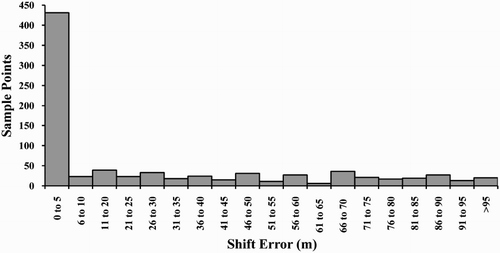
 Figure 1 shows the positional shift in the shoreline derived from two techniques: NDVI and unsupervised classification. Results from the NDVI technique are observed to be better than the classification as the range of variation is greater for the classification technique. Figure 2 shows the error in the actual and model generated shoreline where the error ranges from 0 to 100.07 m and the RMSE is calculated as 31.44 m.

Figure 1. Shifting position of GCPs in NDVI and image classification.

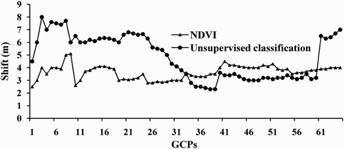
Figure 2. Shift in the position of actual and predicted shoreline.

3.2. Change of shoreline

Clear change in the shoreline of Sagar Island has occurred in many places from 1951 to 2011. There is a clear evidence of decreasing land area or inward shifting of the shoreline. From 1951 to 1990 the greatest changes that occurred were caused by erosion. The period of 1990 to 2011 represents little change where deposition has had some contribution, however the erosion process is strong for the entire period.

The distribution is shown in 2 × 2 km² grids (Figure 3). The boundary of the estuary has experienced constant erosion and deposition, with 1951 depicting the greatest landmass area with significant erosion over the 39 year period to 1990. The scenario changes for 2011 where deposition occurs and about 8 km² landmass has been added to the island. Nevertheless, the total area remains much less compared to the 1951 landmass. Change of area from 1951 to 2011 and statistics of shoreline change are shown in Table 2. Retreat of the shoreline and rate of change was highest from 1951 to 1990 than from 1990 to 2011. The net change of shoreline reveals 48.45 km² loss of land (erosion) from 1951 to 1990, while the last 20 years have experienced much less retreat (1.27 km²). Thus the average change in shoreline was greater from 1951 to 1990.

Figure 3. Distribution of area in grids for different years.

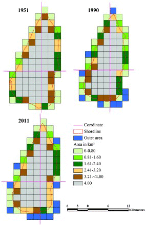
Table 2. Erosion, accretion, net areal changes and statistics of shoreline change of Sagar Island in EPR model.

Area change			Statistics of shoreline changes
	1951–1990 (Km²)	1990–2011 (Km²)	Year (mt/y)	1951–1990 (mt/y)	1990–2011 (mt/y)
Erosion	48.47	6.92	Mean	9.89	0.25
Accretion	0.02	5.65	Max	44.97	29.25
Net change	−48.45	1.27	Min	−1.03	−43.17

The change rate of Sagar Island is shown in the map depicting variation in erosion and deposition with negative and positive values respectively. The rate of change from 1951 to 1990 is 0.032 km² area/year caused by erosion. From 1990 to 2011 the rate of change is 0.005 km² area/year and although the change is quite low, it indicates deposition (main map).

3.3. Prediction of future shoreline

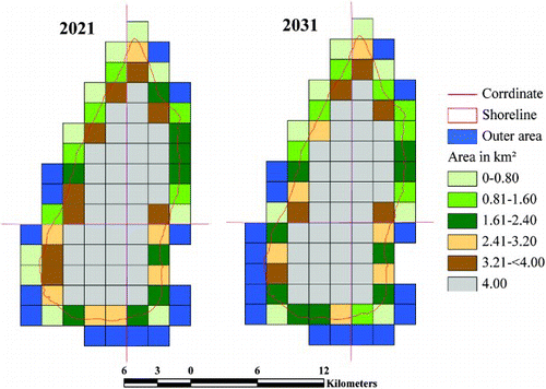
Prediction of future shoreline change or prediction has been performed for 2021 and 2031. The process of erosion has been active and a reduction in area is predicted (Figure 4). In 2021, 14 grids are observed to be outside the land area which have increased to 16 grids in 2031, with the loss of a further 8 km². Constant erosion is predicted leading to the inward shift of the shoreline particularly in the south-west quadrant where wave action is dominant. Predicted results of change rate indicate increase with maximum change in the south-west quadrant (0.06 km²/year) due to erosion (main map).

Figure 4. Predicted area for 2021 and 2031.

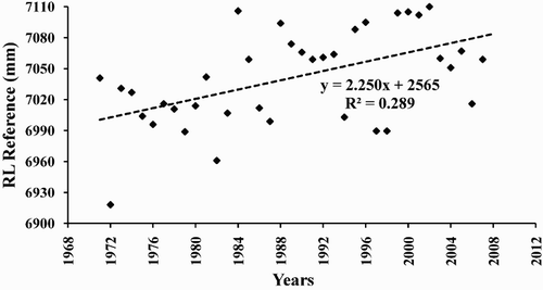
3.4. Impact of sea level on shoreline change

The trend of annual sea level data is represented in Figure 5 with sea level data from the observatory at Haldia station (located about 43 km away). There has been rise in the sea level over the 39 years of data since 1970 with the growth observed to be 2.25 mm year⁻¹. The rise in sea level may be due to an increase in river discharge or sedimentation which has caused a local mean sea level change.

Figure 5. Annual sea level change.

4. Conclusion

Change in the shoreline of Sagar Island has been studied here which indicates an inward shift of the shoreline. There has been a large reduction in the total area of the island due to this change. Constant erosion is seen throughout a period of 60 years from 1951 to 2011. Three images from 1951, 1990 and 2011 have been used in this study with a grid-based analysis performed to obtain a change in boundary. Future prediction also indicates constant erosion and a decrease in land area. Sea level change is a suggested cause for excessive erosion together with cyclonic events. About 55.39 km² has been lost due to erosion which accounts for about 19.41% of the total landmass. Although an increase in area was found from 1990 to 2011, the entire area remains less in comparison to 1951. Higher river discharge coupled with the removal of forest cover and cyclones may be possible causes of erosion and shoreline change.

Software

Mapping of shoreline change and grid-wise analysis was performed in Arc GIS 9.3 and ERDAS Imagine 9.2 has been used for georeferencing. The End Point Rate model is used within ArcGIS.

Acknowledgements

The authors are thankful to the Survey of India, Dehradun and the Global Land Cover Facility (GLCF) for topographic maps and satellite imagery used in the study. We also acknowledge the PSMSL (Permanent Service for Mean Sea Level) records for providing sea level data.

References

- Abd El-Kawya, O. R., Rød, J. K., Ismail, H. A., & Suliman, A. S. (2011). Land use and land cover change detection in the western Nile delta of Egypt using remote sensing data. Applied Geography, 31, 483–494.
- Adarsa, J., Shamina, S., & Biswas, A. (2012). Morphological change study of Ghoramara Island, Eastern India using multi temporal satellite data. Research Journal of Recent Sciences, 1(10), 72–81.
- Backstrom, J. T. (2007). Short-term shoreface changes along a high-energy headland-embayment coast. Journal of Maps, 3, 11–13.
- Bausmith, J. M., & Leinhardth, G. (1997). Middle school students’ map construction: Understanding complex spatial displays. Journal of Geography, 97, 93–107.
- Bertacchini, E., & Capra, A. (2010). Map updating and shoreline control with very high resolution satellite images: Application to Molise and Puglia coasts (Italy). Italian Journal of Remote Sensing, 42, 103–115. doi: http://dx.doi.org/10.5721/ItJRS20104228
- Blum, M. D., & Roberts, H. H. (2009). Drowning of the Mississippi Delta due to insufficient sediment supply and global sea-level rise. Nature Geoscience, 2, 488–491.
- Coleman, J. M., Huh, O. K., & Braud, D. W. Jr. (2008). Wetland loss in world deltas. Journal of Coastal Research, 24(1A), 1–14.
- Cui, B. L., & Li, X. Y. (2011). Shoreline change of the Yellow River estuary and its response to the sediment and runoff (1976–2005). Geomorphology, 127, 32–40. doi:10.1016/j.geomorph.2010.12.001
- Durduran, S. S. (2010). Shoreline change assessment on water reservoirs located in the Konya Basin Area, Turkey, using multitemporal landsat imagery. Environmental Monitoring and Assessment, 164, 453–461.
- Ericson, J. P., Vörösmarty, C. J., Dingman, S. L., Ward, L. G., & Meybeck, M. (2006). Effective sea-level rise and deltas: Causes of change and human dimension implications. Global and Planetary Change, 50, 63–82.
- Fenster, M., Dolan, R., & Elder, J. (1993). A new method for predicting shoreline positions from historical data. Journal of Coastal Research, 9, 147–171.
- Goodchild, M. F. (2001). Metrics of scale in remote sensing and GIS. International Journal of Applied Earth Observation and Geoinformation, 3, 114–120.
- Ingham, A. E. (1974). Hydrography for the surveyor and engineer. London: Blackwell Science Inc.
- Lazarus, E. D., & Murray, A. B. (2011). An integrated hypothesis for regional patterns of shoreline change along the Northern North Carolina Outer Banks, USA. Marine Geology, 281, 85–90.
- Lee, J., & Jurkevich, I. (1990). Shoreline detection and tracing in SAR images. IEEE Transactions in Geosciences and Remote Sensing, 28, 662–668. doi: http://dx.doi.org/10.1109/TGRS.1990.572976
- Li, A., Li, G., Cao, L., Zhang, Q., & Deng, S. (2004). The coast erosion and evolution of the abandoned lobe of the Yellow River Delta. Acta Geographica Sinica, 59(5), 731–737.
- Li, R., Liu, J., & Felus, Y. (2001). Spatial modelling and analysis for shoreline change and coastal erosion monitoring. Marine Geodesy, 24, 1–12.
- Li, X., & Damen, M. C. J. (2010). Shoreline change detection with satellite remote sensing for environmental management of the Pearl River Estuary, China. Journal of Marine Systems, 82, S54–S61. doi:10.1016/j.jmarsys.2010.02.005
- Li, X., & Yeh, A. G. (1998). Principal component analysis of stacked multi-temporal images for the monitoring of rapid urban expansion in the Pearl River Delta. Int. J Remote, 19(8), 1501–1518.
- Lian, L., & Jianfei, C. (2011). Spatial-temporal change analysis of water area in Pearl River Delta based on remote sensing technology. Procedia Environmental Sciences, 10, 2170–2175.
- Maiti, S., & Bhattacharya, A. (2009). Shoreline change analysis and its application to prediction: A remote sensing and statistics based approach. Marine Geology, 257, 11–23.
- Mukhopadhyay, A., Mukherjee, S., Mukherjee, S., Ghosh, S., Hazra, S., & Mitra, D. (2012). Automatic shoreline detection and future prediction: A case study on Puri Coast, Bay of Bengal, India. European Journal of Remote Sensing, 45, 201–213.
- Restrepo, J. D. (2012). Assessing the effect of sea-level change and human activities on a major delta on the Pacific coast of northern South America: The Patía River. Geomorphology, 151–152, 207–223.
- Suresh, P. K., & Sundar, V. (2011). Comparison between measured and simulated shoreline changes near the tip of Indian peninsula. Journal of Hydro-Environment Research, 5, 157–167.
- Survey of India. (NF 45-11). India and Pakistan 1:250000. Series U502.
- Syvitski, J. P. M., & Saito, Y. (2007). Morphodynamics of deltas under the influence of humans. Global and Planetary Change, 57(3), 261–282.
- White, K., & El Asmar, H. (1999). Monitoring changing position of shorelines using Thematic Mapper imagery, an example from the Nile Delta. Geomorphology, 29, 93–105. doi: http://dx.doi.org/10.1016/S0169-555X(99)00008-2
- Yang, X., Damen, M. C. J., & Van Zuidam, R. A. (1999). Satellite remote sensing and GIS for the analysis of channel migration changes in the active Yellow River Delta, China. JAG, 1(2), 146–157.