Ring maps applied to hydrogeological and environmental studies in alluvial aquifers, central Italy

Abstract

Analysis of hydrogeological data of aquifers requires assessment of multiple variables and this is difficult to visualise in a single map with commonly used techniques. Ring maps are presented in this paper as a useful option to overcome this limitation.

Four alluvial aquifers from Central Italy were assessed and are presented as case studies, evaluating the hydrogeological setting, the groundwater chemistry and the distribution of representative contaminants (Boron, Iron, Manganese and Nitrates). The final result is a graphical representation showing the ring maps, which simultaneously depict 12 numerical variables and two other variables: the geographical position and the main lithological properties of the aquifers.

The research indicates that coastal alluvial aquifers show higher contamination when compared to the intramontane alluvial aquifers. Boron is exclusively present in the coastal alluvial aquifers where maximum concentrations are associated with the uprising of deeper saline groundwater with a chloride-sodium chemistry. Iron and manganese are generally associated and their presence is inversely correlated to that of nitrates. The presence of Nitrates is less common in the intramontane aquifers.

The ring maps presented in this paper have been effectively used as a geovisualisation tool for multivariate hydrogeological and environmental data. The technique simultaneously and clearly shows several variables in one single graphical representation.

Keywords:

• hydrochemistry
• geovisualisation
• groundwater contamination
• ring map
• hydrogeology

1. Introduction

The use of Geographical Information Systems (GIS) has grown exponentially over recent years. This has made the production and use of maps one of the most widespread and effective ways to visualise, synthesise and communicate spatial information. The choice of the most appropriate visualisation method is fundamental especially when dealing with the representation, interpretation and communication of large heterogeneous datasets. The importance of georeferencing is testified by the fact that estimates indicate that 80% of all generated digital data are geospatially referenced (MacEachren & Kraak, 2001).

The use of maps is widespread in hydrogeology, however, common methods of data visualisation only allow a small number of variables to be shown at any one time. Hydrochemical analysis of aquifer systems generally involves assessing several variables, including major ions (Calcium, Magnesium, Sodium, Potassium, Chloride, Bicarbonates and Sulphates), physico-chemical parameters (temperature, pH, electrical conductivity and REDOX potential) and possible contaminant concentrations. This information is appropriately contextualised only if it is related to the geographical and hydrogeological setting.

Hydrochemical and environmental data are normally shown numerically in tables and graphs. This approach is suitable for organising and synthesising information but can be difficult to read and also do not provide a geographical context to the data. The choice of representing data with tables and graphs is generally motivated by lack of more advanced visualisation techniques which are effective, easy to apply and functional for the geovisualisation of extensive multivariate datasets.

Ring maps have been used in this study as a tool for representing hydrogeological and environmental data that is commonly available to professionals with a technical/scientific background and that commonly operate as hydrogeologists or land quality experts for the characterisation and remediation of contaminated sites. These types of maps have already been effectively used for the representation of epidemiological data (Battersby, Stewart, Fede, Remington, & Mayfield-Smith, 2011; Stewart et al., 2011) and time series datasets (Ankerst, Keim, & Kriegel, 1996; Bale et al., 2007; Huang, Govoni, Choi, Hartley, & Wilson, 2008; Zhao, Forer, & Harvey, 2008). They require the use of a base map at the centre of the image which is then surrounded by a series of concentric rings, each showing a different variable.

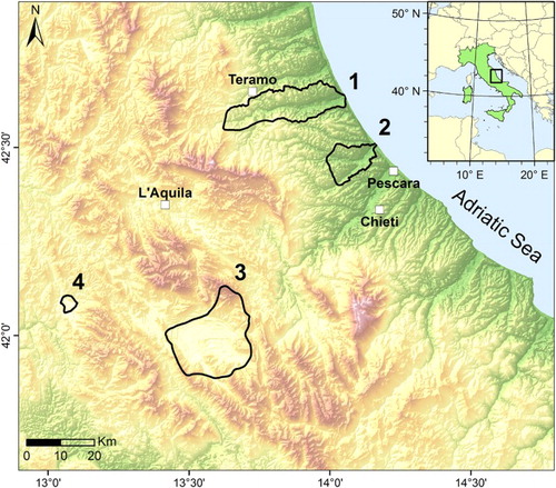
Alluvial aquifers in Central Italy have been used as representative examples in this research (Figure 1), i.e. the coastal alluvial aquifers of the Vomano and Saline Rivers (Maps 1 and 2 in the Main Map) and the intramontane alluvial aquifers of the Fucino and Oricola plains (Maps 3 and 4 in the Main Map).

Figure 1. Location of the coastal and intramontane alluvial aquifers. (1) Vomano alluvial aquifer; (2) Saline alluvial aquifer; (3) Fucino intramontane alluvial aquifer; (4) Oricola intramontane alluvial aquifer).

2. Methods

The ring maps were prepared in two distinct phases. The initial phase involved the collection of the data and materials necessary for the hydrogeological and hydrochemical analysis. The geological characteristics of the aquifers were defined, with particular reference to lithologies and geometry. The groundwater chemistry was then investigated using the data of the ‘Diffuse Pollution’ Regional Project provided by ARTA Abruzzo (Regional Agency for Environmental Protection) (Agenzia Regionale per la Tutela dell'Ambiente, Progetto Regionale ‘Inquinamento Diffuso’, unpublished data, 2011/2012) and the data of Plan for the Protection of Waters provided by the Abruzzo Region (Regione Abruzzo, Piano di Tutela delle Acque, unpublished data, 2010/2011). The same data were used and partially discussed in Palmucci and Rusi (2013, 2014).

Data from a total of 107 groundwater monitoring points were analysed. These locations are represented by 55 and 35 monitoring points respectively distributed within the alluvial valley of the Vomano and Saline Rivers, while 11 and 6 monitoring points respectively distributed within the Fucino and Oricola plains. Analysis of the major ions, the physico-chemical parameters (measured in the field) and the concentration of some contaminants (Iron, Manganese, Boron and Nitrates) was undertaken for each monitoring point. The four contaminants were selected as they often exceed the Concentration Limit of Contamination (CLC) (Table 1) imposed by current Italian Legislation (Italian Republic, 2001, 2006).

Table 1. Summary of the selected contaminants and the colours used in the main map.

^aConcentration Limit of Contamination.

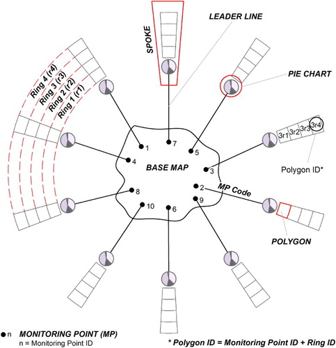
The second phase involved the actual construction of the ring maps; each one of these representations required a central base map showing the monitoring locations and surrounded by a number of spokes corresponding to the number of monitoring locations. Each spoke is constructed of a series of concentric polygons having the shape of a circular sector and used to represent a different variable (Figure 2). Each ring thus shows the representation and distribution of a variable. The ring maps in this research have also been supplemented with pie charts to represent the chemistry of the major ions. Each monitoring point is connected to its corresponding spoke by means of a leader line along which the code of the monitoring point is reported (Figure 2).

Figure 2. Schematic diagram of Ring Map. The image shows all the elements constituting the Ring Map. The different spokes include polygons showing concentrations of contaminants and related pie charts representing major ions hydrochemistry. Each spoke is connected to the corresponding monitoring point by means of a leader line along which the code of the monitoring point is reported. The identifier of the monitoring point and of the ring constitutes the unique identifier of each polygon.

Widely available interoperable software packages were used to construct the ring maps. An external database was designed and implemented for hydrochemical data storage and referencing to map polygons.

Despite the existence of several methods for construction of ring maps (Lee, 2014; Ta-Chien, Chien-Min, & Yung-Mei, 2013), in this research, the base structures of the ring maps were defined within the CAD environment for its flexibility and customisability. Thus the construction of the polygons is extremely fast as it allows the selection of the number of circular sectors to be displayed based on the number of monitoring points. It is also possible to select the dimensions of the polygons as well as their distance based on the number of monitoring points that need to be represented. For the representative maps of this research, the dimensions of the polygons were fixed while their distances were varied providing an indication on the density of the monitoring points.

The base structure of the ring maps was subsequently imported in to a GIS where a series of topological functions were applied to construct the spokes. The positioning of the leader lines around the base maps were selected respecting the geographical position of each individual monitoring point and by minimising overlap and line length.

The attributes of the polygons which constitute the circular sectors were defined in such a way that each polygon has a unique identifier (ID) based on the progressive number of the ring and on the ID of the monitoring location (Figure 2). The external database storing the hydrochemical data was connected with the GIS. Different colours were applied to polygons to represent the range of concentrations of the individual analytes selected for this research (Table 1).

The colour schemes were selected based upon the recommendations of Brewer (2005). A divergent scheme was selected for representing contaminant concentration, while major ions in the pie charts, were represented using a spectral scheme to make it easier to see differences between colour symbols.

The pie charts are connected to monitoring locations by leader lines and show the chemistry of the major ions of the groundwater. The charts were constructed using standard Esri ArcGIS tools and the size of the charts is proportional to the salinity of the groundwater (Sum of Anions and Cations). The positions of the pie charts and labels of the monitoring points were selected in such a way that it does not compromise the readability of any constituting elements of the ring maps.

The geolithological properties of the alluvial aquifers represented on the base maps provide an indication of the groundwater-aquifer interactions. However, any type of information which can be displayed in 2D, can be used as a base map. The selection of the type of data to display in the base map depends on the objectives of the work and, most importantly, on the scale of the representation.

The final ring maps presented in this research simultaneously show 12 numerical hydrochemical variables together with other two context variables, the geographical position and the main geolithological characteristics of the representative alluvial aquifers.

3. Hydrogeological setting

The intramontane alluvial basins are located in flat areas, at lower elevations than the surrounding carbonate mountains. Starting from the Pliocene, these basins were filled with detritic and alluvial deposits sourced from weathering of the surrounding carbonate mountains (Desiderio, D'Arcevia, Nanni, & Rusi, 2012). The deposits have thicknesses varying up to maximums of more than 1000 m (Burri & Petitta, 2004) and are characterised by an extremely variable permeability depending upon granulometry. This heterogeneity within the basins controls groundwater flows mainly occurring within multi-layered aquifer systems. These aquifers are bounded by low permeability deposits that locally determine semi-confined conditions (Petitta, 2009). Recharge is related in part to drainage from the surrounding carbonate structures and in part to direct infiltration from precipitation.

The coastal alluvial aquifers are located along the piedemont areas between the Appennine Mountains and the Adriatic Coast. They are mainly constituted by gravelly-sandy deposits with a silty-clayey matrix and locally by silty-clayey and silty-sandy levels and lenses. The thickness is variable and the discontinuous and heterogeneous nature of the deposits guarantees hydraulic connection between levels of different permeability. These systems can thus be considered as large and multilayered aquifers which are bounded both laterally and at the base by the clayey deposits of the Plio-Pleistocene substrate. The discharge capacity of the alluvial deposits tends to increase downstream, proportionally with the increase of their thicknesses up to about 50 m in coastal zones (Desiderio, Ferracuti, & Rusi, 2007; Desiderio, Nanni, & Rusi, 1999, 2003; Rusi & Tatangelo, 2010; Rusi, Tatangelo, & Crestaz, 2004). The recharge is mainly related to water exchanges with rivers flowing from the Apennine Mountains, especially through paleorivers, but also to rainfall net infiltration and locally to surface and subsurface contributions from the surrounding hills.

The groundwater chemistry (i.e. hydrochemical facies) of the alluvial aquifers is mostly calcium-bicarbonate (Ca-HCO₃). However, calcium-sulphate (Ca-SO₄) and sodium-chloride (Na-Cl) hydrochemical facies are also common (Desiderio, Nanni, Rusi, & Vivalda, 2001; Desiderio & Rusi, 2004).

Groundwater chemistry is generally compatible with the nature of the lithologies which constitute the aquifer systems. The sodium-chloride facies within the coastal valleys aquifers are connected to the uprise, mainly through fault and fracture systems, of saline groundwater trapped in argillaceous deposits of the Plio-Pleistocene substrate (Desiderio, Rusi, & Tatangelo, 2010). These facies can also be related to saline intrusion near the coast (Desiderio & Rusi, 2003).

Both types of aquifer systems, along intramontane basins and coastal valleys, are exploited for civil, industrial and agricultural purposes by means of withdrawal wells.

4. Hydrochemical and environmental characteristics based on the interpretation of the Ring Maps

A hydrochemical and environmental study undertaken with traditional analytical tools requires the evaluation of several outputs. Geological and hydrogeological maps, locations of monitoring points and classification diagrams (e.g. Piper and Schoeller-Berkaloff diagrams), are considered to identify the different groups of groundwater. Tables and charts would be used to assess the presence and severity of contamination while chemical maps usually display the spatial distribution of contaminant concentrations.

The hydrochemical characteristics of the different aquifers can be assessed by a single visual representation using the ring maps. These maps provide the advantage of being able to develop a single representation, where the data can be viewed as a whole.

The maps clearly show the different distribution, density and concentrations of monitoring points between the intramontane basins with respect to coastal valleys. The qualitative status of groundwater within the coastal alluvial aquifers is generally worse, with large zones affected by higher concentrations and even locally contaminated as evident by many monitoring points, showing concentrations above limits imposed by current Italian Legislation.

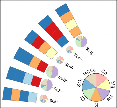
In Maps 1 and 2 in the Main Map it is evident the predominant hydrochemical facies of groundwater in the coastal alluvial aquifers is Ca-HCO₃. However there is locally a significant presence of Na-Cl facies. The dimensions of the pie charts indicates that groundwater with Na-Cl facies have the highest mineral content (Figure 3).

Figure 3. Example of the hydrochemistry of representative monitoring locations. SL4, SL40 and SL8 indicate bicarbonate-calcium groundwater, while SL7, SL48 and SL 39 are typical of groundwater with a chloride-sodium facies. The dimensions of the pie charts clearly indicate that chloride-sodium groundwater are related to an higher mineralisation compared to that of locations characterised by bicarbonate-calcium facies.

Analysis of the geological characteristics displayed in the different base maps clearly reveals that the hydrochemistry generally reflects the lithological properties of the deposits that constitute the aquifers. The presence of monitoring points with a Na-Cl hydrochemical facies is an anomaly that cannot be fully explained considering the lithological properties alone. These facies could be explained considering the uprise of deeper saline groundwater or with saline intrusion along the coastline (Desiderio et al., 2001; Desiderio & Rusi, 2003).

The representative contaminant concentrations are quite widespread in both of the coastal alluvial aquifers (Maps 1 and 2 in the Main Map). Iron and Manganese (Ring 2 and 3 respectively) are intimately related to each other and are often both detected in groundwater samples.

The ring maps clearly show that there is no relationship between the presence of Iron and Manganese and the hydrochemical facies of the groundwater samples. There is, instead, an inverse correlation between these two metals and Nitrates (Ring 4). This is probably due to redox processes within groundwater systems that determine the conditions in which either Nitrates or Iron and Manganese can be found (Berner, 1980; Guffanti, Pilla, Sacchi, & Ughini, 2010; McMahon & Chapelle, 2008; Van Cappellen & Wang, 1996).

This aspect is particularly evident in the north-eastern areas of the Saline River valley (Map 2 in the Main Map), where there are several monitoring locations with very high concentrations of Iron and Manganese and very low concentrations of Nitrates. However, there are a few exceptions in both of the coastal alluvial aquifers, although they are more numerous in the Vomano River valley (examples are VO30, VO49 and VO71 in Map 1 as well as SL12, SL41 and SL46 in Map 2). The presence of Iron and Manganese is clearly more widespread in the Saline River valley where the eastern areas towards the coast show the highest levels of contamination.

Boron (Ring 1) is a widespread contaminant in both of the coastal alluvial aquifers. The maximum observed concentrations are always associated with Na-Cl facies (VO41 and VO74 in Map 1; SL7, SL10, SL39, SL45 and SL48 in Map 2) with few exceptions (VO63 and VO71 in Map 1; SL49 in Map 2). Low Boron concentrations are generally associated to high concentrations of Nitrates.

The dominant hydrochemical facies within the intramontane alluvial aquifers is Ca-HCO₃, although there are monitoring points with Na-Cl facies (Maps 3 and 4 in the Main Map), particularly distributed in the central areas of the Oricola basin (Map 4 in the Main Map).

Boron is never associated with Na-Cl facies, as opposed to observed conditions within the coastal alluvial aquifers. This contaminant is never observed in high concentrations within the intramontane aquifers.

Iron and Manganese, which are always associated even in these areas, are frequently detected and are independent of the hydrochemical facies. The limited presence of Nitrates is also quite evident even though these areas are subject to intensive agricultural activities.

The most likely origin of Iron and Manganese in groundwater is associated with the presence of these metals in the overlying soils, where the two metals are often present in the form of oxides and hydroxides (Bradl, 2005; Cornell & Schwertmann, 2006). Under favourable physico-chemical conditions (ORP/pH), these two metals leach from the soil towards the underlying aquifer (Brennan & Lindsay, 1998; Schwab & Lindsay, 1983).

The ring map presented in this research clearly highlights that the maximum Boron concentrations are observed at monitoring points characterised by strongly mineralised groundwater with a sodium-chloride hydrochemistry (Na-Cl facies), located at significant distances from the coastline.

A more in-depth analysis, which takes into account the hydraulic gradients, the concentrations of the dissolved ions and the ion ratios (SO₄/Cl, Na/Cl e B/Cl), is presented in Palmucci and Rusi (2014). The work undertaken by these authors indicates that the higher concentrations of boron are not associated with saline intrusion but rather with mixing processes between more shallow groundwater and deeper connate groundwater that is enriched with sodium, chloride and boron.

5. Applicability of the method

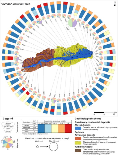
The ring maps have proven to be an effective and versatile technique for the visualisation of multivariate hydrogeological and environmental data. The time taken to construct the maps is rewarded by the possibility of providing a clear and easily interpretable simultaneous visualisation of a large number of hydrochemical and environmental variables. The attached Main Map displays four representative case study areas where a simultaneous visual representation of 12 numerical hydrochemical and environmental variables is overlaid on top of the hydrogeological setting. The ring maps of the Vomano River valley (Map 1 in the Main Map), showing 55 monitoring points, has been reported in Figure 4 as a representative example of these type of visual representations.

Figure 4. Ring Map of the Vomano River alluvial aquifer. The central map shows the geo-lithological properties of the aquifer system, while the pie charts show the hydrochemistry of major ions. The rings represent the concentrations of four representative contaminants, i.e. Nitrate, Manganese, Iron and Boron from the inside towards the outside. Contaminants concentrations are proportional to Concentration Limit of Contamination imposed by current Italian legislation.

The results of the research generally indicate that the hydrochemistry reflects the interactions between the groundwater and lithological properties of the aquifers. In fact, the predominant calcium-bicarbonate facies is related to the lithology of the hosting aquifers.

The alluvial aquifers of the Adriatic Coastal area are characterised by higher levels of contamination with respect to those of the intramontane basins. Iron and Manganese are generally associated and their presence is inversely correlated to the presence of Nitrates. The most contaminated areas are found in the eastern areas of the Saline River plain. Iron and Manganese do not show any correlation with the hydrochemical facies of the groundwater while Boron is clearly correlated to Na-Cl facies. The highest concentrations of Boron are observed in strongly mineralised groundwater samples with a sodium-chloride chemistry that are located at great distances from the coast.

Nitrate concentrations are extremely high in the Vomano River aquifer with concentrations frequently above legislative limits, while they have lower concentrations in the Saline River aquifer with only a few locations exceeding the legislative limit. The presence of Boron and Nitrates is limited in the intramontane aquifers, even though these areas are subject to intensive agricultural activities.

Ring maps present contamination data as point data as opposed to other methods of representation such as contour maps that instead present the data continuously. Consequently, the disadvantage of not visualising continuous data is balanced by the advantage of not visualising interpolated data.

A single ring map may not be sufficient to adequately represent the groundwater contamination in those cases where the hydrogeological setting is particularly complex (e.g. multilevel or overlying aquifers) or where multilevel sampling is required. In such cases, the solution may be to use several ring maps or alternatively add additional features to a single ring map. However, in the latter case, there is a risk of making the final product difficult to interpret. The number of spokes is essentially governed by the number of monitoring points that need to be represented on the ring map. A high number of monitoring points would require an excessive reduction in the size of the spokes although, there are references in literature where up to 350 points have been used (Battersby et al., 2011). The only solution in such cases is to increase the size of the representation with the risk of making it less practical.

6. Conclusions

The representation of large multivariate datasets typical of hydrogeological and environmental studies always presents limitations associated with the creation and visualisation of maps that are easy to read and interpret. The ring maps, as those investigated and presented in this study, are an effective and innovative tool for the visualisation of hydrochemical and environmental data. Four of the most common contaminants are presented for the groundwater of the Central Adriatic regions of Italy and have been effectively assessed based on interpretation of the ring maps implemented in this research. The structure of the ring maps is versatile and easy to manage. The most demanding and time consuming element of the implementation process is the construction and layout of the leader lines around the base maps. Once this process is completed, the variables or contaminants to be visualised and their respective ranges can be rapidly selected. The number of visualised contaminants can be increased simply by increasing the number of rings. The range intervals for the concentrations can also be increased thus providing more detailed information. All these choices are based on the purpose of the ring maps, as increasing the rings and the details of the representation, increases the difficulty of interpretation.

Another aspect to be highlighted is the reduced dimensions of the final representation. The ring maps can be included in the most common printing formats without compromising the readability.

Software

The ring maps were developed in AutoCAD LT2011 from Autodesk and ESRI ArcGIS 10, with data stored within a Microsoft Access database. Labelling was defined using the ESRI ArcGIS Maplex Label Engine. The final layout and editing were also undertaken within ESRI ArcGIS 10.

Acknowledgements

The authors wish to thank the Abruzzo Region ‘Servizio Qualità delle Acque’ and the Regional Agency for the Protection of the Environment (Agenzia Regionale per la Tutela dell'Ambiente – ARTA, ‘Progetto Inquinamento Diffuso’) for having made available the groundwater quality data. The authors are also grateful to reviewers for their comments and suggestions.

References

- Ankerst, M., Keim, D. A., & Kriegel, H. P. (1996). ‘Circle Segments’: A Technique for Visually Exploring Large Multidimensional Data Sets. Proc. Visualization'96, Hot Topic Session, San Francisco, CA, 1996.
- Bale, K., Chapman, P., Barraclough, N., Purdy, J., Aydin, N., & Dark, P. (2007). Kaleidomaps: A new technique for the visualization of multivariate time-series data. Information Visualization, 6(2), 155–167.
- Battersby, S. E., Stewart, J. E., Fede, A. L. D., Remington, K. C., & Mayfield-Smith, K. (2011). Ring maps for spatial visualization of multivariate epidemiological data. Journal of Maps, 7(1), 564–572. doi:10.4113/jom.2011.1182
- Berner, R. A. (1980). Early diagenesis: A theoretical approach (No. 1). Princeton University Press, Princeton, New Jersey, USA.
- Bradl, H. (Ed.) (2005). Heavy metals in the environment: Origin, interaction and remediation (Vol. 6). Academic Press, Waltham, Massachusetts, USA.
- Brennan, E. W., & Lindsay, W. L. (1998). Reduction and oxidation effect on the solubility and transformation of iron oxides. Soil Science Society of America Journal, 62(4), 930–937. doi:10.2136/sssaj1998.03615995006200040012x
- Brewer, C. A. (2005). Designing better maps: A guide for GIS users. ESRI Press, online library.
- Burri, E., & Petitta, M. (2004). Agricultural changes affecting water availability: From abundance to scarcity (Fucino Plain, central Italy). Irrigation and Drainage, 53(3), 287–299. doi:10.1002/ird.119
- Cornell, R. M., & Schwertmann, U. (2006). The iron oxides: Structure, properties, reactions, occurrences and uses. John Wiley & Sons, online library.
- Desiderio, G., D'Arcevia, C. F. V., Nanni, T., & Rusi, S. (2012). Hydrogeological mapping of the highly anthropogenically influenced Peligna Valley intramontane basin (Central Italy). Journal of Maps, 8(2), 165–168, doi:10.1080/17445647.2012.680778
- Desiderio, G., Ferracuti, L., & Rusi, S. (2007). Structural-stratigraphic setting of middle Adriatic alluvial plains and its control on quantitative and qualitative groundwater circulation. Memorie Descrittive della Carta Geologica d'Italia, 76, 147–162.
- Desiderio, G., Nanni, T., & Rusi, S. (1999). Gli acquiferi delle pianure alluvionali centro adriatiche [The aquifers of the central Adriatic alluvial plains]. Quaderni di Geologia Applicata, 2, 21–30.
- Desiderio, G., Nanni, T., & Rusi, S. (2003). La pianura del fiume Vomano (Abruzzo): Idrogeologia, antropizzazione e suoi effetti sul depauperamento della falda [The Vomano river plain (Abruzzo-central Italy): Hydrogeology, anthropic evolution and its effects on the depletion of the unconfined aquifer]. Bollettino della Società Geologica Italiana, 122(3), 421–434.
- Desiderio, G., Nanni, T., Rusi, S., & Vivalda, P. (2001). The mineralized springs of the Marche and Abruzzi foredeep, central Italy: Idrochemical and tectonics features. Proceedings of Tenth International Symposium of Water – Rock Interaction, Villasimius (Italy), 1, 493–496.
- Desiderio, G., & Rusi, S. (2003). Il fenomeno dell'intrusione marina nei subalvei della costa abruzzese [The freshwater-saline water relations in the coastal zones of the unconfined acquifers of Abruzzo alluvial plains]. Quaderni di Geologia Applicata, 10(1), 17–31.
- Desiderio, G., & Rusi, S. (2004). Idrogeologia e idrogeochimica delle acque mineralizzate dell'Avanfossa Abruzzese Molisana [Hydrogeology and hydrochemistry of the mineralized waters of the Abruzzo and Molise foredeep (Central Italy)]. Bollettino della Società Seologica Italiana, 123(3), 373–389.
- Desiderio, G., Rusi, S., & Tatangelo, F. (2010). Caratterizzazione idrogeochimica delle acque sotterranee abruzzesi e relative anomalie [Hydrogeochemical characterization of Abruzzo groundwaters and relative anomalies]. Italian Journal of Geosciences, 129(2), 207–222.
- Guffanti, S., Pilla, G., Sacchi, E., & Ughini, S. (2010). Caratterizzazione della qualità e origine delle acque sotterranee del lodigiano mediante metodi idrochimici ed isotopici [Characteriziation of the quality and origino f groundwater of lodigiano (Northern Italy) with hydrochemical and isotopic instruments]. Italian Journal of Engineering Geology and Environment, 10(1), 65–78. doi:10.4408/IJEGE.2010-01.O-05
- Huang, G., Govoni, S., Choi, J., Hartley, D. M., & Wilson, J. M. (2008). Geovisualizing data with ring maps. ArcUser, Winter, 54–55.
- Italian Republic. (2001). Legislative Decree 2 February 2001, n. 31. ‘Attuazione della direttiva 98/83/CE relativa alla qualità delle acque destinate al consumo umano’. Gazzetta Ufficiale Repubblica Italiana, n. 52 del 03/03/2001. Retrieved from http://www.camera.it/parlam/leggi/deleghe/01031dl.htm
- Italian Republic. (2006). Legislative Decree 3 April 2006, n. 152. ‘Norme in materia ambientale’. Gazzetta Ufficiale Repubblica Italiana n. 88 del 14/06/2006. Retrieved from http://www.camera.it/parlam/leggi/deleghe/06152dl.htm
- Lee, M. (2014). Create Ring Maps using PyQGIS Script. Retrieved from http://www.onspatial.com/2014/01/qgis-create-ring-maps-using-pyqgis.html?spref=tw
- MacEachren, A. M., & Kraak, M. J. (2001). Research challenges in geovisualization. Cartography and Geographic Information Science, 28(1), 3–12. doi:10.1559/152304001782173970
- McMahon, P. B., & Chapelle, F. H. (2008). Redox processes and water quality of selected principal aquifer systems. Ground Water, 46(2), 259–271.
- Palmucci, W., & Rusi, S. (2013). Origin and distribution of iron, manganese and boron in the Abruzzo region groundwaters. Hydrogeochemical survey on the Saline sample area. Rendiconti Online della Società Geologica Italiana, 22, 222–224.
- Palmucci, W., & Rusi, S. (2014). Boron-rich groundwater in Central Eastern Italy: A hydrogeochemical and statistical approach to define origin and distribution. Environmental Earth Sciences. doi:10.1007/s12665-014-3384-5
- Petitta, M. (2009). Impact of farming on the water resources of the Fucino Plain (Central Italy). Italian Journal of Engineering Geology and Environment, 9(2), 59–90. doi:10.4408/IJEGE.2009-02.O-05
- Rusi, S., & Tatangelo, F. (2010). Conceptualization, modelling and management of alluvial aquifers: Case studies of Sangro and Vomano plains (central Italy). Memorie Descrittive della Carta Geologica d'Italia., 90, 245–266.
- Rusi, S., Tatangelo, F., & Crestaz, E. (2004). The hydrogeological conceptualisation and well fields management of the Vomano Valley (Abruzzo, central Italy) using groundwater numerical modelling. Geologia Tecnica e Ambientale, 4, 5–22.
- Schwab, A. P., & Lindsay, W. L. (1983). The effect of redox on the solubility and availability of manganese in a calcareous soil. Soil Science Society of America Journal, 47(2), 217–220. doi:10.2136/sssaj1983.03615995004700020008x
- Stewart, J. E., Battersby, S. E., Lopez-De Fede, A., Remington, K. C., Hardin, J. W., & Mayfield-Smith, K. (2011). Diabetes and the socioeconomic and built environment: Geovisualization of disease prevalence and potential contextual associations using ring maps. International Journal of Health Geographics, 10, 18. Retrieved from http://www.biomedcentral.com/content/pdf/1476-072X-10-18.pdf
- Ta-Chien, C., Chien-Min, W., & Yung-Mei, L. (2013). Looking at Temporal Changes. Retrieved from http://www.esri.com/~/media/Files/Pdfs/news/arcuser/1013/ringmap.pdf
- Van Cappellen, P., & Wang, Y. (1996). Cycling of iron and manganese in surface sediments; a general theory for the coupled transport and reaction of carbon, oxygen, nitrogen, sulfur, iron, and manganese. American Journal of Science, 296(3), 197–243.
- Zhao, J., Forer, P., & Harvey, A. S. (2008). Activities, ringmaps and geovisualization of large human movement fields. Information Visualization, 7(3–4), 198–209.