Mapping cost distance using air traffic data

ABSTRACT

Recent trends in transport and communication infrastructures have had a profound impact on the spatial organization of the world city network, which have long been of interest to geographers. Considering the former issue, our study is based on previous works on air transport geography and world city network studies. We introduce a new method to map the gap between geographical distance and cost distance by using air traffic data. In this paper, we created an international database for a large number of world cities and developed a way to map cost distance using conventional and Geographic Information System-based mapping techniques. The main result of this work is a set of maps showing the cost distances of world cities, which can be used as a significant source of information by world city network analysis.

KEYWORDS:

• Cost distance
• world city
• air traffic
• transport
• innovative cartography

1. Introduction

From the second half of the twentieth century, the development of transportation and information technologies (the so-called time–space shrinking technologies) has had a profound impact on the spatial organization of an increasingly globalized society and facilitated integration by allowing the flows of people, goods, and information through various systems (Dicken, 2007; Rodrigue, Comtois, & Slack, 2006). The ever-growing spread of civilian air travel since the 1930s significantly accelerated the process of spatial integration (Massey, 1991, 1993) and radically altered concepts of distance and has led to the world getting ‘shrunk’ dramatically. Although the world has indeed shrunk in relative terms – the absolute distance between two points did not change, but relative distances decreased (Warf, 2006) – but this shrinkage is highly uneven (Dicken, 2011). This is partly because air transport that facilitates the flows and changes in the world is unevenly distributed in space and is concentrated in certain nodes (world cities), thus these nodes remain hierarchically organized at global and national levels (Beaverstock, Smith, & Taylor, 2000; Knox & Taylor, 1995; Sassen, 2001; Taylor, Catalano, & Walker, 2002a). In the aftermath of the global economic crisis, a restructuring is taking place in the power geometry of world cities, new growth poles ascend, while the geopolitical situation and the importance of these nodes are changing – just as cities’ position in the world city hierarchy. Consequently, some of the world cities are being pulled closer together in relative or cost terms, while others are being left behind (Dicken, 2011). So the question may arise: How far is it from point A to point B in relative terms?

Based on the ever-increasing role of air transport and the high-level interest in world cities we think it is time to investigate the connection between cost distance and geographical distance and determine how far point A from point B is in the world city universe from the perspective of air transport. So the purpose of our research is to introduce a new method to measure and visualize the gap between cost distance and geographical distance.

In the first half of the research, we developed a database for a large number of world cities that included data on distance and cost of airline connections. In the second part, these data were mapped using Geographic Information System (GIS)-based mapping techniques. The results were cost distance maps which offer a visual representation of the gap between cost distance and geographical distance.

2. Methods

2.1. Determination of the analytical units and data mining method

We started our study with the selection of our analytical units (world cites). From a preliminary database using academic literature (Beaverstock, Taylor, & Smith, 1999; Clarke, 2005; Short, Kim, Kuss, & Wells, 1996; Taylor, Walker, Catalano, & Hoyler, 2002b) and international statistics (ACI, 2006; GaWC, 2008, www.citypopulation.de), the 100 most important world cities were selected using a ranking based on the population of the cities (www.citypopulation.de reflecting the situation of 1 January 2010), their GaWC rank (GaWC, 2008), and the passenger traffic of the cities’ airports (ACI, 2006). In those cities where more than one airport is handling notable scheduled air passenger traffic, the passenger numbers of each airport were summed.

In the next phase of the research air traffic connection data between world city-pairs were queried. First of all, the already existing ticket price databases (e.g. APTCO Airline Tariff Publishing Company, BACK Aviation O&D-lux Origin – Destination Fare Data) were examined. However, we realized that they were not freely available for researchers, do not contain sufficient information, and are also incomplete. Thus, we queried data from the Internet, which is also accepted in academic literature (Bilotkach, 2010; Burghouwt, van der Vlier, & de Wit, 2007; Dobruszkes, 2006, 2009; Law, Leung, Denizci Guillet, & Lee, 2011; Lijesen, Rietveld, & Nijkamp, 2002; Zook & Brunn, 2005, 2006). We investigated some of the main available ticket search engines (Expedia, Kayak, Opodo, Orbitz, Travelocity) and our decision fell on www.orbitz.com which is a leading online travel agency connected to a major computer reservation system called Worldspan. Although Orbitz has some deficiencies – for example, low-cost airlines were absent – our choice fell on it, because it displayed the most applicable information and had the most user-friendly interface for a manually made data query. Although, we have to note that the results might have been different for other search engines – even if price deviations were rather small by our comparison queries – but it did not affect the mapping process (in which creation was our main purpose). Since this is a methodological paper, we consider this as an acceptable deficiency, but in further research the involvement of low-cost carriers would be necessary to get a real picture of the actual situation.

To obtain the necessary data we performed two manual queries to minimize the distorting effects of tourism in air traffic. The queries were constructed for round-trip flights, but we took into consideration that some kind of fare asymmetry can be observed between city-pairs on round-trip flights depending on from which city the journey starts (flying A-B-A may be cheaper than B-A-B). So, for example, the London–Rio de Janeiro return and the Rio de Janeiro–London return were queried on the same day and treated separately during the study. That flights between certain city-pairs – same route but different departure city – are differently priced reflects that, for example, Rio de Janeiro is having a different position in the cost space of London than London in the cost space of Rio Janeiro. So due to fare asymmetry, we will get different maps in the case of A-B-A than B-A-B, which gives us additional information about cost spaces and cost distances of world cities.

The first query was on 1 February 2010 for flights leaving on 1 March 2010 (Monday) and returning on 8 March 2010 (Monday), while the second was on 5 June 2010 for flights leaving on 2 August 2010 (Monday) and returning on 9 August 2010 (Monday). The selected cities also served as departure cities and as destination cities. The data collection concerned traffic data between each of the selected 100 cities, which contained the lowest fares (economy seats), flight time, the departure-, transfer-, and arrival airports, as well as the fares of the shortest flights.

2.2. Tools for visualization of cost distance

To visualize and handle the queried data we used a GIS system, the ESRI ArcGIS 10 and its tools. During the mapping process we used two extensions: the Military Analyst Tool (MAT) and Tools for Graphics and Shapes.

2.2.1. Military analyst tool (MAT)

The ESRI ArcGIS Military Analyst is a freely downloadable extension, which incorporates a suite of tools (e.g. Raster and Vector Map Tool, Data Management Tools, Geodesy Tools, etc.) to enhance the effectiveness of core ArcGIS and geospatial intelligence analyst (ArcGIS Military Analyst Brochure, 2005). In our analysis we wanted to portray geodesically properly the connecting lines of the geographical location and the relative (calculated) location of the cities represented in the survey. We found that the Geodesy Tools is suitable to meet our expectations. It allows users to create great circle and rhumb lines and also enables to specify two coordinates and generate a great circle route, a rhumb line, or a geodesic route, while the geodesy calculator also calculates bearing, azimuth, distance, and the end coordinate (ArcGIS Military Analyst Brochure, 2005). Using these tools (Geodesy Calculator) we can determine the distance between two points and their azimuth, which enables us to connect the points with geodesy lines while we eliminate the date line problem.

2.2.2. Tools for graphics and shapes

During our research we found that the Military Analysts’ Geodesy Tools are suitable to visualize the cost distance between our analytical units, but in our case it had some deficiencies. Due to our large database it would have taken a lot of time to calculate the necessary data in each city-pair. So we looked for an application, which speeded up the working process. We choose the Tools for Features and Shapes application. This application is part of a package called Tools for Graphics and Shapes developed by Jennes Enterprises and is freely downloadable from their website. From this extension, we used the Calculate Geometry tool.

This function calculates a wide variety of geometric attributes of point, multipoint, polygon, and polyline feature classes, including lengths, centroids, and areas calculated on sphere or spheroid. Some of these attributes may also be calculated using the standard ArcGIS ‘Calculate Geometry’ function, however this function provides many attributes that the standard ArcGIS function does not offer, and this function can add new fields to the attribute table automatically if necessary. (Jennes, 2011, p. 18)

Using this tool we speeded up the working (calculation) process, and with the MAT we could display the cost distance values on the maps.

2.3. Calculation of cost distance

In order to calculate cost distance we needed three parameters: ticket price, geographical distance of the world city-pairs, and the price per distance parameter the cost of 1 km travel from city ‘A’ to city ‘B’ by air. Ticket price was already queried and geographical distance (based on inter-city great circle distance) was defined by using the Calculate geometry application from ArcGIS 10 and the cities coordinates from Google Earth. Using inter-city great circle distance as a measure of geographical distance is customary in academic literature (e.g. Hazledine & Bunker, 2013; Zook & Brunn, 2006), although we have to mention that great circle distances diverge from distances really flown by planes because of technical, geophysical, and geopolitical constraints. This can cause a gap between cost distance and geographical distance (due to planes flying longer routes than great circle ones), but our purpose was to use a standard database (great circle distance between city-pairs does not change but flight distance is different in each case due to the aforementioned factors), so considering the literature we assumed that this gap is incorporated into the ticket price and inter-city great circle distance is an appropriate measure of city distance.

Doganis (2002) found that the relationship of air transport cost to distance is curvilinear and not a straight line, as transport costs normally decrease per unit distance traveled (Knowles, 2006; Taaffe, Gauthier, & O'Kelly, 1996). By the determination of the price per distance value we had to take into consideration that fares increase with distance but not in a linear way, so this value – similarly to the flight distance – may differ in each city-pair (e.g. due to the different pricing methods of the airlines, distance flown, aircraft type, etc.), so we could not determine it individually.

Considering this issue, in order to define the price per distance parameter, we decided to categorize our city-pairs and calculate average price per distance values assuming that the cost of 1 km air travel might not greatly differ in the defined categories. Using academic literature (AEA, 2004; Francis, Dennis, Ison, & Humphreys, 2007) – according to flight duration and flight distance – we defined four distance levels and classified our city-pairs into these four categories (Table 1). Then, for each category we calculated the average of the city-pair distances and so did we with the ticket prices. Next, in each category average ticket prices were divided by average city-pair distances and the results were the four price per distance parameters. So the costs of 1 km travel in short-haul routes were 0.256 USD, in medium-haul routes 0.160 USD, in long-haul routes 0.140 USD, and in ultralong-haul routes 0.122 USD. Finally, we calculated the cost distances by dividing the ticket prices with the price per distance parameters.

Table 1. Categorization of distance levels in air transportation.

Flight zone	Time (h)	Distance (km)	Price per distance parameters (USD)
Short-haul	<3	<2000	0.256
Medium-haul	3–6	2001–4000	0.160
Long-haul	6–12	4001–9500	0.140
Ultralong-haul	>12	>9500	0.122

Note: (AEA, 2004; Francis et al., 2007) and own calculation.

2.4. Mapping of cost distance

At the beginning of the mapping process we compiled the initial database (Table 2) and started to compute the ‘cost distance points’ on the sphere. Firstly, using the WGS84 projection system we depicted the departure city and the arrival cities on a vector-based world map (Figure 1). In the second step, we used the MAT/Geometry/Table to Line tool and connected the departure point with the arrival points (Figure 1). This tool converts a table (text file, dbase table, Excel file, etc.) containing coordinate and other required data to a feature class, where the output features are two-point line features (ESRI, 2011). In the third step based on the feature class saved in the previous step, great circle distance (Spheroidal length) and azimuth (Start azimuth) were calculated using the Graphics and Shapes/Tools for Features and Shapes/Calculate Geometry tool. After this move, great circle distance was displayed on the map with the MAT/Geometry/Table to Geodesy Line tool. This tool converts a table (text file, dbase table, Excel file, etc.) containing coordinate and other required data to a feature class, where the output features are polyline features representing geodesic, great circle, or rhumb lines (ESRI, 2011). Meanwhile, great circle distance values of the city-pairs were used to calculate the cost distance values (see in the previous chapter). In the fourth step based on the feature class saved in Step 3, the latitude and longitude coordinates of the ‘cost distance points’ were determined using Graphics and Shapes/Tools for Features and Shapes/Calculate Geometry tool, and with the MAT/Geometry/Table to Line tool we connected these points with the arrival points. In the fifth step, the ‘cost distance points’ were depicted on the map with different (green) coloring. In the sixth step based on the feature class saved in Step 4, great circle distance and azimuth were calculated between the arrival points and ‘cost distance points’ using Graphics and Shapes/Tools for Features and Shapes/Calculate Geometry tool again. Applying the MAT/Geometry/Table to Geodesy Line tool, negative or positive shifts of ‘cost distance points’ according to geographical position of the cities were displayed on the map with different colors. In the case of positive shift, the relative position of the cities is closer to the departure point than their geographical position, while in the case of the negative shifts the relative position of the city is farther than their geographical position (while the length of the lines gives the size of the positive/negative shift).

Figure 1. Mapping phases of cost distance.

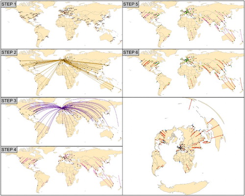
Table 2. Example of the initial database.

START_CITY	S_LAT_Y	S_LON_X	END_CITY	E_CITY_CODE	E_LAT_Y	E_LON_X
London	51.487911	−0.177998	Amsterdam	AMS	52.373043	4.894833
London	51.487911	−0.177998	Atlanta	ATL	33.795700	−84.349228
London	51.487911	−0.177998	Beijing	BJS	39.906193	116.388039

Note: Edited by the authors.

Abbreviations in the headings are the follows: START_CITY – name of the departure city; S_LAT_Y – Latitude coordinate of the departure city; S_LON_X – longitude coordinate of the departure city; END_CITY – name of the arrival city; E_CITY_CODE – Airport code of the arrival city; E_LAT_Y – Latitude coordinate of the arrival city; E_LON_X – Longitude coordinate of the arrival city.

Finally, we came to the conclusion that the equirectangular projection makes it impossible to compare values for different cities, so we changed our map projection and used an equidistant azimuthal projection centered on the departure city. With this projection the great circles through the central city will be straight lines and all distances passing through the departure point will be correctly displayed and can be unequivocally compared on our map. In order to improve the readability of the map, we indicated the four distance categories using isochrones on the final map (see Main Map in supplementary material) and used a base map generalized for smaller scales (base map downloaded from http://www.naturalearthdata.com).

3. Conclusion

This research presents a method to map the gap between cost distance and geographical distance by using air traffic data. We created an international database for large number of world cities and developed a way to map cost distance using conventional and GIS-based mapping techniques. The main result of this work is the creation of a mapping process and a set of maps showing the cost distances of world cities, which allows people to see a relative picture of the world where world cities would be located if only air ticket price would matter.

The methodological results of the research are that it synthesizes the data collecting, analysation, and mapping methods of various disciplines and eliminates some critical elements (e.g. lack of origin/destination information in standard data sources, data sources contain information only on international flows) of the previous studies (see in Derudder & Witlox, 2008). Although, it should be noted that the paper mostly brings methodology, but further methodological issues (e.g. low-cost airlines not considered, planes not following great circles) have to be addressed. We also emphasize that to conduct a deeper and wider empirical analysis further works on the input data are needed. We hope that our study will encourage further research in this topic and raise further interest among geographers and researchers from other disciplines.

Map design

The preview map represents the cost distance of world cities considering the cheapest flights from London in 2010. On this map, the geographical position of world cities is represented by black circles, while the colored lines show shifts of the relative position of the world cities according to cost distance. On the map, red lines are representing the positive shifts of the relative position of the world cities compared to their geographical position. In these cases, the ticket price was cheaper than the two cities’ geographical distance would imply, so the relative position of the city is closer than its geographical position, and the length of the line gives the size of the positive shift. In the case of the blue lines quite opposite tendencies can be observed, as the ticket prices were more expensive than the city-pairs geographical distance would imply, so the relative position of the city is farther than their geographical position, and the length of the line gives the size of the negative shift.

Software

Several software packages were used in the development of our cost distance maps. The air traffic data were collected and maintained in a Microsoft Excel and LibreOffice Calc database. ESRI ArcGIS 10 Desktop was used for all the GIS operations and for mapping the cost distance. In addition, Corel Draw X7 was used for further cartographic enhancement.

Disclosure statement

No potential conflict of interest was reported by the authors.

ORCID

Gábor Dudás http://orcid.org/0000-0001-9326-8337

References

- Airports Council International (ACI). (2006). World Air Traffic Report 2006. ACI World Headquarters Geneva, Switzerland.
- ArcGIS Military Analyst Brochure. (2005). GIS tools for the defense and intelligence communities. Redlands: ESRI. Retrieved November 29, 2013, from http://downloads.esri.com/support/whitepapers/other_/military-analyst.pdf
- Association of European Airlines (AEA). (2004). AEA Yearbook 2004. Brussels: Association of European Airlines (P VI-9).
- Beaverstock, J. V., Smith, R. G., & Taylor, P. J. (2000). World city network: A new metageography? Annals of the Association of American Geographers, 90, 123–134. doi: 10.1111/0004-5608.00188
- Beaverstock, J. V., Taylor, P. J., & Smith, R. G. (1999). A roster of world cities. Cities, 16, 445–458. doi: 10.1016/S0264-2751(99)00042-6
- Bilotkach, V. (2010). Reputation, search cost, and airfares. Journal of Air Transport Management, 16, 251–257. doi: 10.1016/j.jairtraman.2010.01.002
- Burghouwt, G., van der Vlier, A., & de Wit, J. (2007). Solving the lack of price data availability in (European) aviation economics? ATRS World Conference, Berkeley, CA.
- Clarke, D. (2005). Urban world/global city (2nd ed.). London: Routledge.
- Derudder, B., & Witlox, F. (2008). Mapping world city networks through airline flows: context, relevance, and problems. Journal of Transport Geography, 16, 305–312. doi: 10.1016/j.jtrangeo.2007.12.005
- Dicken, P. (2007). Global shift – Mapping the changing contours of the world economy (5th ed.). New York: Guilford Press.
- Dicken, P. (2011). Global shift – Mapping the changing contours of the world economy (6th ed.). New York: Guilford Press.
- Dobruszkes, F. (2006). An analysis of European low-cost airlines and their networks. Journal of Transport Geography, 14, 249–264. doi: 10.1016/j.jtrangeo.2005.08.005
- Dobruszkes, F. (2009). New Europe, new low-cost air services. Journal of Transport Geography, 17, 423–432. doi: 10.1016/j.jtrangeo.2009.05.005
- Doganis, R. (2002). Flying off course: The economics of international airlines (3rd ed.). New York: Routledge.
- ESRI ArcGIS Desktop 9.3 Help. (2011). Retrieved November 29, 2013, from http://webhelp.esri.com/arcgisdesktop/9.3/index.cfm?TopicName=Table%20to%20Line%20%28Military%20Analyst%29
- Francis, G., Dennis, N., Ison, S., & Humphreys, I. (2007). The transferability of the low-cost model to long-haul airline operations. Tourism Management, 28, 391–398. doi: 10.1016/j.tourman.2006.04.014
- GaWC – Globalization and World Cities Study Group and Network. (2008). The world according to GAWC 2008. Loughborough University. Retrieved January 11, 2010, from http://www.lboro.ac.uk/gawc/world2008t.html
- Hazledine, T. & Bunker, R. (2013). Airport size and travel time. Journal of Air Transport Management, 32, 17–23. doi: 10.1016/j.jairtraman.2013.06.003
- Jennes, J. (2011). Tools for Graphic and Shapes. Flagstaff: Jennes Enterprises. Retrieved November 29, 2013, from http://www.jennessent.com/downloads/Graphics_Shapes_Online.pdf
- Knowles, R. D. (2006). Transport shaping space: Differential collapse in time-space. Journal of Transport Geography, 14, 407–425. doi: 10.1016/j.jtrangeo.2006.07.001
- Knox, P., & Taylor, P. J. (1995). World cities in a world system. Cambridge: Cambridge University Press.
- Law, R., Leung, R., Denizci Guillet, B., & Lee, H. A. (2011). Temporal changes toward fixed departure date. Journal of Travel and Tourism Marketing, 28, 615–628. doi: 10.1080/10548408.2011.598740
- Lijesen, M. G., Rietveld, P., & Nijkamp, P. (2002). How do carriers price connecting flights? Evidence from intercontinental flights from Europe. Transportation Research Part E: Logistics and Transportation Review, 38, 239–252. doi: 10.1016/S1366-5545(02)00008-X
- Massey, D. (1991). A global sense of place. Marxism Today, 38, 24–29.
- Massey, D. (1993). Power-geometry and a progressive sense of place. In J. Bird, B. Curtis, T. Putnam, G. Robertson, & L. Tickner (Eds.), Mapping the futures: Local cultures, global change (pp. 60–70). London: Routledge.
- Rodrigue, J. -P., Comtois, C., & Slack, B. (2006). The geography of transport systems. London: Routledge.
- Sassen, S. (2001). The global city: New York, London, Tokyo. Princeton, NJ: Princeton University Press.
- Short, J. R., Kim, Y., Kuss, M., & Wells, H. (1996). The dirty little secret of world city research. International Journal of Regional and Urban Research, 20, 697–717. doi: 10.1111/j.1468-2427.1996.tb00343.x
- Taaffe, E. J., Gauthier, H. L., & O'Kelly, M. (1996). Geography of transportation (2nd ed.). Englewood Cliffs, NJ: Prentice Hall.
- Taylor, P. J., Catalano, G., & Walker, D. R. F. (2002a). Measurement of the world city network. Urban Studies, 39, 2367–2376. doi: 10.1080/00420980220080011
- Taylor, P. J., Walker, D. R. F., Catalano, G. & Hoyler, M. (2002b). Diversity and power in the world city network. Cities, 19(4). 231–241. doi: 10.1016/S0264-2751(02)00020-3
- Warf, B. (2006). Time-space compression. In B. Warf (Ed.), Encyclopedia of human geography (pp. 491–494). London: SAGE.
- Zook, M. A., & Brunn, S. D. (2005). Hierarchies, regions and legacies: European cities and global commercial passenger air travel. Journal of Contemporary European Studies, 13, 203–220. doi: 10.1080/14782800500212459
- Zook, M. A., & Brunn, S. D. (2006). From podes to antipodes: Positionalities and global airline geographies. Annals of the Association of American Geographers, 96, 471–490. doi: 10.1111/j.1467-8306.2006.00701.x