The surficial and subglacial geomorphology of western Dronning Maud Land, Antarctica

ABSTRACT

The surficial and subglacial geomorphology of ∼220,000 km² of western Dronning Maud Land (WDML), Antarctica, is presented at a scale of 1:750,000. The mapped area includes the Stancomb-Wills Glacier north of 75°25′S and follows the grounded ice margin to the Jutulstraumen Ice Stream at the Prime Meridian. Mapping of subglacial geomorphology builds upon recent methodological advances that use optical and passive satellite imagery of the ice surface to infer major elements of the subglacial topography. The hypothesised geomorphological map reveals an alpine glacial landscape at, and surrounding, every nunatak region, inferred through the presence of subaerial and subglacial cirques, arêtes and closely spaced hanging valleys. A series of subglacial troughs are found to intersect the main Jutulstraumen–Penck troughs. The map is aimed at helping analyse patterns and processes of landscape evolution within WDML and provides greater detail of erosion patterns associated with former ice flow patterns.

KEYWORDS:

• Antarctica
• Dronning Maud Land
• landscape evolution
• subglacial geomorphology
• subglacial mapping

1. Introduction

Detailed knowledge of the subglacial landscape of Antarctica can inform interpretations of former ice sheet characteristics, including ice flow regime and basal thermal regime, by providing an insight into the patterns of glacial erosion that formed the topography (Jamieson et al., 2014; Jamieson, Sugden, & Hulton, 2010). The long-term evolution of the East Antarctic Ice Sheet (EAIS) over the last 34 Ma is only understood from global records or from records near the ice sheet margin (McKay et al., 2012; Miller, Wright, & Browning, 2005; Naish et al., 2001). However, away from the ice margin, the potential of the sub-ice landscape to be interpreted as a record of past ice dynamics has not yet been fully exploited (Jamieson et al., 2014). Therefore, if different landscapes of glacial erosion (Sugden, 1974, 1978; Sugden & John, 1976) can be classified through mapping, and if these are then associated with ice sheets of various scales that have existed in the past, a clearer picture of the fluctuations of the EAIS can be revealed.

The recent development and availability of remotely sensed data sets of the surface and bed of the Antarctic continent (e.g. Fretwell et al., 2013; Haran, Bohlander, Scambos, Painter, & Fahnestock, 2014; Jezek, Curlander, Carsey, Wales, & Barry, 2013; Scambos, Haran, Fahnestock, Painter, & Bohlander, 2007) have meant that the subglacial landscape can be examined in more detail than has hitherto been possible because variability in the data often reflects changes in the morphology and roughness of the ice sheet bed (Crabtree, 1981; Jezek, 1999; Rose et al., 2014; Ross et al., 2014). However, directly surveyed bed topography data are of varied resolution and remain poorly constrained in many regions. Indeed, even the recently published BEDMAP2 (Fretwell et al., 2013) contains sparse or even no ice thickness measurements in some areas: between Recovery and Support Force Glaciers and in Princess Elizabeth Land, for example, direct ice thickness measurements are entirely absent (Fretwell et al., 2013). Western Dronning Maud Land (WDML; Figure 1) is comparatively well covered by direct measurements of the bed elevation, but data still remain somewhat sparse for some areas (Figure 2), with distances between data points ranging between less than a kilometre to greater than 20 km, which has made interpretation of the landscape, its processes of evolution and thus past ice sheet dynamics and extent challenging.

Figure 1. Study area and its major geomorphological and geological locations. The yellow region delineates the area within which it was possible to map geomorphological features in WDML and the background data are the MODIS MOA (Haran et al., 2005). The inset shows the location of the study area.

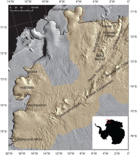
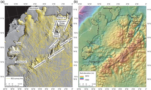
Figure 2. Current knowledge of bed topography in WDML. (a) Survey line locations (yellow) used in BEDMAP2 bed topography (Fretwell et al., 2013). Note the relatively sparse data over the Borg Massif, Kirwan Escarpment and Vestraumen; (b) Corresponding BEDMAP2 bed elevation product for WDML. Note that it is difficult to identify small-scale topographic features in the subglacial landscape. Boxes indicate locations of detailed mapping shown in other figures.

A recent innovative mapping technique (Ross et al., 2014) involves manipulating ice surface imagery to infer subglacial topography, and was used successfully to characterise the subglacial geomorphology of the Ellsworth Subglacial Highlands. This study aims to apply (and develop) the mapping methodology outlined in Ross et al. (2014) to WDML in order to produce the first detailed surficial and subglacial geomorphological map of the region.

2. Study area

Dronning Maud Land (DML) is located between 20°W and 45°E in East Antarctica and this study focusses on the western part of the region in an area totalling ∼220,000 km² (Figure 1). The study area includes the Stancomb-Wills Glacier north of 75°25′S and follows the grounded ice margin to the Prime Meridian, terminating at the Jutulstraumen ice stream. WDML consists of several nunatak groups that form a broad escarpment and several smaller subglacial mountain ranges, and these have been modified extensively by tectonic, fluvial and glacial processes dating back to continental rifting in the Late Mesozoic (Ferraccioli, Jones, Curtis, & Leat, 2005; Näslund, 2001). These processes, however, are currently not well constrained spatially or chronologically. Upland areas of the territory are highly likely to have been a nucleation site for early development of Antarctic ice (DeConto & Pollard, 2003; Jamieson & Sugden, 2008), and they are likely to act as a key pinning point of the present-day EAIS. Modelling suggested that the majority of ice within DML is cold-based at present (Näslund, Fastook, & Holmlund, 2000). Given the potential for landscape preservation under such non-erosive ice, it is possible that the subglacial DML uplands may contain evidence for earlier, smaller ice conditions, with the possibility that landforms could have been preserved since the 14 Ma expansion of Antarctic ice or even EAIS inception at 34 Ma. Such interpretations have been made at other areas of high subglacial relief within Antarctica where features implying widespread alpine glaciation (including arêtes, hanging valleys, glacial troughs and high elevation corries) have been identified, which could not have formed under the ice sheet at its present-day configuration (Bo et al., 2009; Jamieson et al., 2014; Rose et al., 2013; Sugden & Denton, 2004; Young et al., 2011). The major glaciological and geological features in the study area are reviewed below.

2.1. Escarpments

The ∼410-km-long escarpment that dominates the study area runs SW to NE and starts at the Heimefrontfjella, a range which extends for approximately 160 km of the escarpment front and consists of three distinct mountain groups (Worsfold, 1967). These mountains obstruct ice flow and create an abrupt transition from the polar plateau (>2500 m a.s.l.) to a coastal, lower lying region (>1500 m a.s.l.; Van den Broeke et al., 1999). The large subglacial mountains have been inferred to continue beneath the ice, based on observation of uneven wrinkles in the surface (Holmlund, 1993; Marsh, 1985; Whillans & Johnsen, 1983). The Kirwan escarpment runs almost contiguously from the Heimefrontfjella as a straight SW to NE ridge; it is also marked by a steep step descending from 2800 to 2000 m. The Neumayer Cliff area constitutes the end of the Kirwan escarpment.

2.2. Ice streams

In WDML, the mountain ranges restrict ice flow from the continental interior, and therefore ice drainage through these mountains often reflects local snowfall and ice transport (Pohjola, Hedfors, & Holmlund, 2004). The Jutulstraumen ice stream lies in a deep valley in subglacial bedrock (Bentley, 1987) and is bordered by the Ahlmann Ridge and Borg Massif to the west. It is the largest ice stream of the region, draining an area of ∼124,000 km² (Swithinbank, 1988), most of which is sourced via the SE branch and not through the distinctive Penck trough (Rignot, Mouginot, & Scheuchl, 2011), the bed of which is a few hundred metres below sea level (Fretwell et al., 2013). The Schytt glacier, to the west of Jutulstraumen, is also situated in a deep subglacial trough which extends south and proceeds to join Penck trough some 200 km downstream. Vestraumen, between the Heimefrontfjella and Vestfjella to the west, drains a significant proportion of ice from the coastal region of DML (Rignot et al., 2011).

2.3. Geology

Geological structure and lithology of the bed are key controls on rates and patterns of glacial erosion (Sugden, 1978) and so it is important to understand the geology of the region. The Pencksökket and Jutulstraumen glaciers conceal a major crustal boundary between two distinctive terranes within WDML: the Grunehogna and Maudheim Provinces (Groenewald, Moyes, Grantham, & Krynauw, 1995; Moyes, Krynauw, & Barton, 1995). At least three major rock units of differing age can be found within these two provinces (Figure 3; Spaeth & Fielitz, 1987).

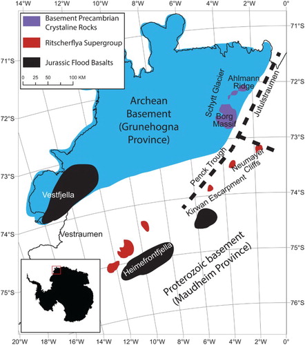
Figure 3. Contextual geological map of the nunatak geology in WDML. The map shows the two distinct provinces (Grunehogna and Maudheim) as well as the location of Jurassic flood basalts, Precambrian basement rock exposures and the sedimentary-volcanic sequences of the Ritscherflya Supergroup. Also shown are the inferred grabens of the Jutulstraumen–Pencksökket triple junction (thick dashed lines). Modified from Ferraccioli et al. (2005) using maps by Spaeth and Fielitz (1987).

2.3.1. Grunehogna province

The Grunehogna Province is an Archaean to mid-Proterozoic cratonic fragment which includes the Ahlmann Ridge and Borg Massif and extends to the northern Vestfjella. It consists of ∼3 Ga granitic basement rocks overlain by an undeformed ∼1.2 Ga sequence of sedimentary and volcanic rocks known as the Ritscherflya Supergroup (Groenewald et al., 1995; Moyes et al., 1995). This has been interpreted as a sequence of shallow marine, tidal and alluvial fan deposits, into which numerous tholeiitic sills are intruded, dated to ∼1.1 Ga and which is capped by the Straumsnutane lavas of a similar age (Moyes et al., 1995; Wolmarans & Kent, 1982). Näslund (2001) suggested that the separated nunatak groups of the Vestfjella, the Borg Massif and the Ahlmann ridge are inselbergs formed by the retreat of the main escarpment following passive continental rifting; this is discussed below.

2.3.2. Maudheim province

The Maudheim Province includes a metamorphic orogenic belt of mid-late Proterozoic age, extending from the Heimefrontfjella to the Sverdrupfjella (Groenewald, Grantham, & Watkeys, 1991; Moyes, Barton, & Groenewald, 1993) and making up the main escarpment region of the study area. Nunataks of the escarpment consist largely of crystalline basement metamorphic rocks of Precambrian age (Spaeth & Fielitz, 1987), predominately gneiss, dated at ∼1.1 Ga in the Heimefrontfjella (Jacobs, Bauer, Spaeth, Thomas, & Weber, 1996). At some localities within the Kirwan Escarpment, less resistant shales and sandstones of Permian age (the Amelang Plateau Formation) have been deposited onto the basement Precambrian metamorphic rocks (Aucamp, Wolmarans, & Neethling, 1972; Faure & Mensing, 2011). Jurassic tholeiitic basalts are also present within the sequence, and correspond in age with the main phase of Karoo volcanism in southern Africa (Duncan, Hooper, Rehacek, Marsh, & Duncan, 1997; Ferraccioli et al., 2005). These basalts are referred to as the Kirwan Volcanics and are widespread at the Vestfjella and in some parts of the Heimefrontfjella (Faure & Mensing, 2011). Figure 3 shows the extent and location of these basalts in the study area.

It is suggested that the Jutulstraumen and Penck troughs, as well as their corresponding ‘triple junction', are Jurassic grabens that resulted from crustal extension during Gondwana break-up and corresponding Karoo volcanism, representing an Antarctic continuation of the East African Rift (Grantham & Hunter, 1991). The main period of uplift probably also occurred during continental break-up in the Late Mesozoic (Emmel, Jacobs, Crowhurst, Austegard, & Schwarz-Schampera, 2008) as DML formed a passive continental margin that was elevated during the rifting process and which underwent associated escarpment retreat (Näslund, 2001).

3. Methods

Initially, surficial features were mapped in order to provide a context for the mapping of subglacial features. Subglacial mapping was carried out based on the assumption that patterns in ice surface morphology often reflect the distribution of subglacial ridges and valleys (Ross et al., 2014). The utility of ice surface imagery for mapping subglacial landscapes, and its close match to topography mapped by ice radar data where such data exist, has already been shown for the Ellsworth Highlands, West Antarctica (Ross et al., 2014). In WDML the subglacial ridge and valley patterns identified using this technique are morphologically similar to typical mountainous terrains from other parts of the globe, further indicating that it is highly likely that a real topographic signal is reflected in the ice surface data sets. The specific criteria used to map subglacial features are discussed in more detail in Section 3.3. In some areas the ice surface topography is very smooth and this inhibited the detection of major subglacial features, which dictated the extent of the study area (Figure 1).

Line and polygon shapefiles were produced for each feature type using a geographic information system (GIS), ArcGIS 10.2, into which individual features were manually digitised by using either raw or processed remote sensing data sets as a guide. The process and data are described below.

3.1. Remote sensing data sets

Surficial geomorphological and glaciological features were mapped using LANDSAT imagery obtained from the Global Land Cover Facility (GLCF, 2013), the LANDSAT Image Mosaic of Antarctica (LIMA) (Bindschadler et al., 2008; LIMA, 2008), the Moderate resolution Imaging Spectroradiometer Mosaic of Antarctica (Haran, Bohlander, Scambos, Painter, & Fahnestock, 2005; Scambos et al., 2007) and the Radarsat Antarctica Mapping Project (RAMP) Ice Surface Digital Elevation Model (DEM) version 2 (Liu, Jezek, Li, & Zhao, 2001). Subglacial features were mapped through manipulation of the RAMP Image Mosaic of Antarctica version 2 (Jezek et al., 2013) and the Moderate resolution Imaging Spectroradiometer (MODIS) Mosaic of Antarctica (MOA) data set (Haran et al., 2005; Scambos et al., 2007), whilst contextual information was provided by the Making Earth System data records for Use in Research Environments (MEaSUREs) ice velocity data set (Rignot et al., 2011) and BEDMAP2 (Fretwell et al., 2013) data sets. Locations of research stations were imported from the online Antarctic Digital Database (ADD; SCAR, 2013) and ice shelves were imported from the BEDMAP2 geodatabase (Fretwell et al., 2013). Table 1 gives the specifications of these data sets including their resolution.

Table 1. Summary of data sources used in geomorphological mapping.

Name	Description	Resolution	Source
LIMA	A true-colour, high-spatial resolution image of Antarctica constructed from nearly 1100 Landsat-7 ETM^+ scenes	240 m	Bindschadler et al. (2008); LIMA (2008)
GLCF LANDSAT imagery	Individually selected Landsat-7 ETM^+ scenes. Bands 3, 2 and 1 were downloaded and pan sharpened with the panchromatic band 8 to give high-resolution, true-colour images	15–30 m	GLCF (2013)
BEDMAP2	Ice thickness and bed elevation data. Bed elevation is determined by subtracting ice thickness measurements at 24.8 million points from ice surface elevations	1 km	Fretwell et al. (2013)
MODIS MOA	A digital image map of Antarctic surface morphology derived from composites of 260 MODIS orbit swaths	125 m	Haran et al. (2005); Scambos et al. (2007)
RAMP Ice Surface DEM version 2	Continent-wide DEM derived primarily from ERS-1 satellite radar altimeter data, the US Geological Survey and the ADD	200 m	Liu et al. (2001)
RAMP AMM-1 Image Mosaic of Antarctica version 2	A single image mosaic derived from SAR data acquired over 18 days as part of the first AMM-1 in 1997	125 m	Jezek (1999); Jezek et al. (2013)
MEaSUREs Ice Velocity Map	Antarctic ice velocity derived from Envisat ASAR, ALOS PALSAR, ERS-1/2, RADARSAT-2 and satellite radar interferometry	900 m	Rignot et al. (2011)
Scientific Community on Antarctic Research (SCAR) –ADD	Geographic information layers for incorporation to a GIS. Used for reference in this investigation were grounded ice margin, moraine and exposed bedrock shapefiles	Varies widely depending on resolution of source data	SCAR (2013)

3.2. Mapping of exposed ridges and ice surficial features

Subaerial features, including nunatak ridges and exposed cirques, were mapped as solid lines; where these continued beneath the ice surface a dashed line symbol was adopted (see Section 3.3). Surficial mapping was carried out primarily on LIMA and other LANDSAT scenes because true colour enabled differentiation between bedrock, blue ice areas and other structural glaciological features that could not otherwise be identified. Alternative LANDSAT imagery had to be used instead of LIMA tiles for a large proportion of the surficial mapping exercise because several LIMA scenes were grainy and unusable. A slight offset was noted between the two data sets which varies regionally (up to ∼100 m), meaning that features mapped onto LIMA tiles are slightly offset from those mapped onto the GLCF imagery. However, the offset is minor and had a negligible effect on the map. In places, higher resolution satellite imagery was available via Google Earth and this was used to supplement the mapping of features that could not be accurately identified from the LANDSAT imagery.

3.2.1. Nunatak geomorphology

Distinctive subaerial hollows were mapped as cirques if they followed the general criteria for identifying the features set out by Evans and Cox (1974), that is, ‘a hollow, open downstream but bounded upstream by the crest of a steep slope (headwall), which is arcuate in plan around a more gently sloping floor’ (Evans & Cox, 1974; page 151). Smaller features such as moraines were often very difficult to identify at the resolution of the imagery and so were identified through comparison with pre-mapped areal data from the ADD (SCAR, 2013). Ridges were not subdivided because of the difficulty in differentiating arêtes from broader ridges at coarser resolutions.

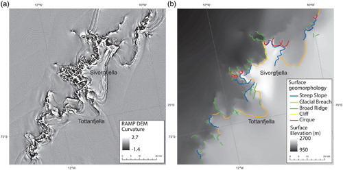
Another difficulty in mapping surficial features was differentiating ridge crests from breaks in slope. This was addressed through raster curvature analysis of the RAMP DEM (Liu et al., 2001). Curvature within a DEM is the rate of change of surface slope whereby high curvature values represent breaks in slope beneath broad ridges and low curvature values represent the ridge tops themselves (Figure 4). This analysis also allowed for the easy identification of glacial breaches where plateau ice overspills along the main escarpment because the breach results in much less abrupt change in curvature. Whilst the DEM has known accuracy issues, with random errors (>4 m) and regionally varying bias (Bamber & Gomez-Dans, 2005), these are not significant enough to be an issue in this exercise. Steep breaks in slope and cliffs were mapped in bold to enable the easy differentiation of plateau areas and broad ridges.

Figure 4. The use of ice surface elevation data for geomorphological mapping. (a) Raster curvature analysis of the RAMP DEMv2 (Liu et al., 2001) at the Heimefrontfjella region; (b) mapped surface geomorphological features and buried glacial breaches. Base data are the RAMP DEMv2.

3.2.2. Ice surface features

Ice surficial features were mapped because they can help identify the nature of the subglacial terrain beneath. Furthermore, they provide a means of contrasting modern ice flow behaviour with past ice flow behaviour as mapped from the subglacial geomorphology. First, using the LIMA data, >2500 areas of blue ice, covering a total of ca. 2550 km², were digitised. This is of interest because the vast majority of blue ice tends to be found directly above the inferred subglacial ridges (Bintanja, 1999). Second, areas of heavy crevassing were mapped because they often correlate with bed structures, acting as a source of restraint to ice flow (Stephenson & Bindschadler, 1990). Crevasse patterns can also be used to infer the location of ice stream margins where fast-moving ice shears past slower moving ice (Vornberger & Whillans, 1990). Furthermore, since they tend to represent regions of fast and extending flow at icefalls (Harper & Humphrey, 1998), they can be representative of a steep subglacial break in slope and drop in elevation. However, the interpretation of subglacial topography from crevassed areas was treated with care because crevasses can be carried down-glacier and become subject to further rotation and bending (Vornberger & Whillans, 1990), meaning that they may not currently be located at the region in which they were initially formed. Visible ice flow lines were mapped because these enable visualisation of the pattern of ice flow direction, which is essential to understanding where warm-based ice is present and thus where erosion could be ongoing (Sugden, 1978). Patterns inferred by flow lines were reinforced by the MEaSUREs ice velocity data set (Rignot et al., 2011).

3.3. Mapping of subglacial features

Subglacial mapping was predominantly carried out following manipulation of the digital ice surface data sets, particularly MODIS MOA imagery (Haran et al., 2005), and synthetic aperture radar (SAR) data from the RAMP Image Mosaic of Antarctica version 2 (Jezek et al., 2013). It is therefore important to note that the subglacial features should be interpreted as inferred features. These data sets were used as base maps and features were mapped following the criteria outlined below.

3.3.1. Subglacial valleys

Ross et al. (2014) revealed that manipulation of MODIS MOA imagery (Haran et al., 2005) can be used to infer subglacial morphology in the Ellsworth Subglacial Highlands. The raster curvature function calculates the second derivative of the surface, thus picking out linear features representing sharp changes in contrast in continuous surface data. This function was applied to the MODIS MOA data in order to identify areas with the most variable surface imagery: Ross et al. (2014) used classified values of >0.05 and <−0.05 for the profile curvature output (curvature parallel to the direction of maximum change) to outline areas representative of underlying ridge features, with values in between often highlighting subglacial valley networks. This assumption builds upon earlier work by Rémy and Minster (1997) who applied curvature analysis in the across-slope direction and found that anomalies displayed at the ice surface relate to bedrock ridges at the coast. We found that the values used for the curvature classification were sensitive to the area of the ice sheet being analysed and were dependent upon the wavelength of surface expression produced as the ice flows over subglacial valleys and ridges. We classified the MODIS MOA imagery at values of >0.03 and <−0.03 in order to resolve the subglacial valley and ridge morphologies in DML. However, we note that in a few parts of DML, the variations at the ice surface were at wavelengths which were too long to enable characterisation of valleys and ridges using this technique. Figure 5 provides an example of where this method successfully identified subglacial ridge lines and Figure 6 demonstrates that, in places, the technique was less effective. In these areas, subglacial valleys were instead best identified manually using unprocessed MODIS MOA imagery, which displayed them more clearly as textural changes on the ice surface.

Figure 5. MODIS MOA and its use for mapping subglacial valleys and troughs. (a) Profile Curvature analysis of MODIS MOA data (Haran et al., 2005) around the Jutulstraumen–Penck trough area; (b) Inferred subglacial valleys and troughs.

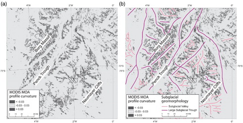
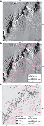
Figure 6. Mapping subglacial valleys around the Kirwan Escarpment. (a) MODIS MOA imagery (Haran et al., 2005) of the eastern Kirwan Escarpment; (b) mapped subglacial valleys by using textural changes on the MODIS MOA data; (c) profile curvature analysis of the same area indicating that features are not always delineated clearly using this method.

3.3.2. Subglacial ridges

Uneven, linear wrinkles and shadows on satellite imagery from DML have previously been attributed to subglacial ridges (Holmlund, 1993; Marsh, 1985; Whillans & Johnsen, 1983), with this interpretation justified by the fact that the features are logical extensions of exposed nunatak ridges. The pattern of ridges extending beneath the ice is remarkably well picked up by the RAMP Antarctica Mapping Mission (AMM)-1 SAR data (Jezek et al., 2013) as areas of higher reflectance (Figure 7).

Figure 7. Subglacial mapping of the Heimefrontfjella. (a) LIMA showing uneven linear features extending from the main escarpment; (b) RAMP AMM-1 Image Mosaic of Antarctica version 2 (Jezek et al., 2013) which has clearly visible linear features which are interpreted as a network of subglacial ridges; (c) Mapping of these ridges and other geomorphological features; (d) Geomorphological features overlain on BEDMAP2 bed topography to illustrate the fit with known topography and the additional topographic detail provided by the mapping.

Interpreting these features as subglacial ridges is supported by Welch and Jacobel (2005), who interpreted areas of bright reflectivity from similar RADARSAT imagery as a signature of angular unconformities resulting from wind erosion as ice deforms over submerged mountain ridges. This was also noted by Paulsen and Wilson (2004), who were able to infer subglacial ridges and faults within the Transantarctic Mountains. As ice flows over subglacial relief, the viscous response of the ice leads to perturbations on the surface (Gudmundsson, 2003; Ross et al., 2014), which may be exploited further by the wind, modifying local accumulation patterns (Bintanja, 1999). With increased ice thickness, the response to subglacial topography is dampened (Ross et al., 2014), explaining the difficulty in mapping any features beyond areas of high relief within the study region.

3.3.3. Other subglacial features

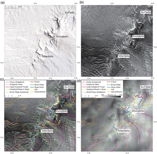
The LANDSAT scenes show several ripple-like features on the ice surface which, when examined in the RAMP AMM-1 SAR data, are not displayed as distinctively as the clearer subglacial ridges. These are most common at the upstream regions of the major ice streams, particularly the Vestraumen. Because they cannot be confidently identified, they are broadly mapped as subglacial breaks in slope. The same symbology was also used for similar features within upland areas where the RAMP AMM-1 SAR imagery indicated that the features were more likely to represent a subglacial slope transition within a mountain range, as opposed to a ridge crest. Mapping of subglacial cirques was tentative and largely informed by the pattern of mapped subglacial ridges because the ‘bowl’ shape of the bed could only be identified in plan view. Where several arête-like ridges converge at higher elevations to form the idealised cirque shape (Evans & Cox, 1974), as visualised using BEDMAP2 (Fretwell et al., 2013) and the RAMP AMM-1 SAR imagery (Jezek et al., 2013), then these were mapped as subglacial cirques.

4. Mapping results

An extensive alpine landscape is inferred through the presence of subaerial and subglacial cirques, arêtes and closely spaced hanging valleys, and is observed at every nunatak region across the study area (Main Map). Where possible, subglacial features were compared against the data in BEDMAP2 (Fretwell et al., 2013). Although BEDMAP2 does not resolve the full detail of the bed topography in this region, we found that the positions of the major subglacial valleys and ridges fit well with those mapped in BEDMAP2 (Figure 7d). However, our map (Main Map) adds significant detail over and above that visible in BEDMAP2.

The features at the main escarpment and those in the vicinity of the Jutulstraumen are briefly described below.

4.1. Escarpment region

Mapping (Main Map) has revealed an extensive pattern of subglacial ridges and valleys across the escarpment region, most notably at the Heimefrontfjella where the extent of the buried mountain range is clearly shown. Significant subglacial valley networks exist on the inland side of the main escarpment and typically form series of parallel and closely spaced hanging valleys over deeper glacial troughs, as well as radial patterns: this is particularly evident at the Kirwan Escarpment. The Neumayer Cliffs, at the north-eastern extent of the escarpment, represent sharp drop-offs from an upstanding plateau; ice spills over these cliffs forming spectacular, heavily crevassed ice falls. The escarpment region is also an excellent location to infer the most recent ice sheet history owing to the impressive occurrence of blue ice areas that occur on the NW facing side, frequently in conjunction with medial and lateral moraines.

4.2. Borg Massif, Ahlmann Ridge and Jutulstraumen

The landscape in the vicinity of the Jutulstraumen Ice Stream exhibits remarkably uniform and large-scale subglacial troughs with a dominant NE trend: the ca.12-km-wide Jutulstraumen–Penck trough is the largest of these and trends NE for ca. 250 km (Main Map). These large subglacial troughs appear to be juxtaposed with a secondary suite of troughs trending SE to NW that includes the SE branch of the Jutulstraumen as well as several larger subglacial valleys that extend from the Neumayer Cliffs and Borg Massif to the Penck and Schytt troughs, respectively.

The Borg Massif, between the Jutulstraumen and Schytt glaciers, incorporates the highest proportion of exposed bedrock in WDML. Several small, dissected plateaux covered by ice caps are present throughout: the largest of these is ca. 30 km² and located along the northern side of the Raudberg valley, a large ca. 40 km trough that dissects the massif. The plateaux are incised by 14 well-developed cirques.

5. Conclusions

A detailed and extensive geomorphological map displaying the surficial and hypothesised subglacial geomorphology and exposed structural glaciology of ∼220,000 km² of WDML has been produced (Main Map). This is the first of its kind for the region and is intended to be useful to further geomorphological, palaeoenvironmental and palaeoglaciological studies in DML. LANDSAT ETM+ data allowed for accurate mapping of areas where bedrock is exposed as nunataks and structural glaciological forms. Subglacial ridges were remarkably well accentuated by the RAMP AMM-1 SAR data set (Jezek et al., 2013), and subglacial valleys were best determined by tracing features across unprocessed MODIS MOA imagery (Haran et al., 2005; Scambos et al., 2007). The profile curvature analysis methodology employed by Ross et al. (2014) in the Ellsworth Mountains was only useful locally within WDML, indicating that the best remote sensing techniques for mapping subglacial topography could vary regionally in Antarctica.

The finalised map (Main Map) allows for an extensive analysis of landscape evolution within WDML because such a comprehensive depiction of the subglacial landscape enables the reconstruction of former ice flow and basal thermal regimes. In turn, this can provide insight into the patterns of glacial erosion that formed the landscape (Jamieson et al., 2010, 2014). Furthermore, as subglacial morphology regulates where ice develops, erodes and flows (Jamieson & Sugden, 2008), it is also a useful constraint for numerical models of ice sheet and climate interaction that may be used to better understand the growth, evolution and stability of the EAIS over the last 34 million years.

Disclosure statement

No potential conflict of interest was reported by the authors.

Software

The data sets described in Table 1 were incorporated as layers in Esri ArcGIS 10.2 in which the map was created. Raster analyses and direct comparison of layers allowed for the identification of the best technique for mapping certain features. Higher resolution satellite imagery available via Google Earth was used to map features that could not be accurately identified from the LANDSAT imagery, with data exported to ArcGIS and incorporated into the map.

Additional information

Funding

This work was carried out as part of a Master's research project in the Department of Geography at Durham University. SSRJ is supported by funding from a Natural Environment Research Council (NERC) Fellowship NE/J018333/1. The geomorphological map data are available upon request from the corresponding author.

References

- Aucamp, A. P. H., Wolmarans, L. T., & Neethling, D. C. (1972). The Urfjell Group, a deformed (?) early Paleozoic sedimentary sequence, Kirwanveggen, western Dronning Maud Land. In R. J. Adie (Ed.), Antarctic geology and geophysics (pp. 557–561). Oslo: Universitetsforlaget.
- Bamber, J. L., & Gomez-Dans, J. L. (2005). The accuracy of digital elevation models of the Antarctic continent. Earth and Planetary Science Letters, 237(3–4), 516–523. doi: 10.1016/j.epsl.2005.06.008
- Bentley, C. R. (1987). Antarctic ice streams: A review. Journal of Geophysical Research: Solid Earth, 92(B9), 8843–8858. doi: 10.1029/JB092iB09p08843
- Bindschadler, R., Vornberger, P., Fleming, A., Fox, A., Mullins, J., Binnie, D., … Gorodetzky, D. (2008). The Landsat Image Mosaic of Antarctica. Remote Sensing of Environment, 112(12), 4214–4226. doi:http://dx.doi.org/10.1016/j.rse.2008.07.006 doi: 10.1016/j.rse.2008.07.006
- Bintanja, R. (1999). On the glaciological, meteorological, and climatological significance of Antarctic blue ice areas. Reviews of Geophysics, 37(3), 337–359. doi:10.1029/1999RG900007
- Bo, S., Siegert, M. J., Mudd, S., Sugden, D., Fujita, S., Xiangbin, C., … Yuansheng, L. (2009). The Gamburtsev mountains and the origin and early evolution of the Antarctic Ice sheet. Nature, 459, 690–693. doi: 10.1038/nature08024
- Crabtree, R. D. (1981). Subglacial morphology in Northern Palmer Land, Antarctic Peninsula. Annals of Glaciology, 2(1), 17–22. doi:10.3189/172756481794352496
- DeConto, R. M., & Pollard, D. (2003). Rapid Cenozoic glaciation of Antarctica induced by declining atmospheric CO2. Nature, 421(6920), 245–249. doi: 10.1038/nature01290
- Duncan, R. A., Hooper, P. R., Rehacek, J., Marsh, J. S., & Duncan, A. R. (1997). The timing and duration of the Karoo igneous event, southern Gondwana. Journal of Geophysical Research: Solid Earth, 102(B8), 18127–18138. doi:10.1029/97JB00972
- Emmel, B., Jacobs, J., Crowhurst, P., Austegard, A., & Schwarz-Schampera, U. (2008). Apatite single-grain (U-Th)/He data from Heimefrontfjella, East Antarctica: Indications for differential exhumation related to glacial loading? Tectonics, 27(6), TC6010. doi:10.1029/2007TC002220
- Evans, I., & Cox, N. (1974). Geomorphometry and the operational definition of cirques. Area, 6(2), 150–153.
- Faure, G., & Mensing, T. M. (2011). Kirwan Volcanics, Queen Maud Land. In G. Faure & T. M. Mensing (Eds.), The transantarctic mountains (pp. 471–489). Dortrecht: Springer.
- Ferraccioli, F., Jones, P. C., Curtis, M. L., & Leat, P. T. (2005). Subglacial imprints of early Gondwana break-up as identified from high resolution aerogeophysical data over western Dronning Maud Land, East Antarctica. Terra Nova, 17(6), 573–579. doi:10.1111/j.1365-3121.2005.00651.x
- Fretwell, P., Pritchard, H. D., Vaughan, D. G., Bamber, J. L., Barrand, N. E., Bell, R., … Zirizzotti, A. (2013). Bedmap2: improved ice bed, surface and thickness datasets for Antarctica. The Cryosphere, 7, 375–393. doi:10.5194/tc-7-375-2013
- GLCF. (2013). Global Land Cover Facility. Retrieved October 6, 2015, from http://www.landcover.org
- Grantham, G. H., & Hunter, D. R. (1991). The timing and nature of faulting and jointing adjacent to the Pencksökket, western Dronning Maud Land, Antarctica. In M. R. A. Thomson, J. A. Crame, & J. W. Thomson (Eds.), Geological evolution of Antarctica (pp. 47–51). Cambridge: Cambridge University Press.
- Groenewald, P. B., Grantham, G. H., & Watkeys, M. K. (1991). Geological evidence for a Proterozoic to Mesozoic link between southeastern Africa and Dronning Maud Land, Antarctica. Journal of the Geological Society, 148(6), 1115–1123. doi:10.1144/gsjgs.148.6.1115
- Groenewald, P. B., Moyes, A. B., Grantham, G. H., & Krynauw, J. R. (1995). East Antarctic crustal evolution: geological constraints and modelling in western Dronning Maud Land. Precambrian Research, 75(3–4), 231–250. doi:10.1016/0301-9268(95)80008-6
- Gudmundsson, H. (2003). Transmission of basal variability to a glacier surface. Journal of Geophysical Research, 108(B5). doi:10.1029/2002JB002107
- Haran, T. M., Bohlander, J., Scambos, T., Painter, T. H., & Fahnestock, M. (2005). MODIS Mosaic of Antarctica (MOA). Boulder, CO: National Snow and Ice Data Center (NSIDC).
- Haran, T. M., Bohlander, J., Scambos, T., Painter, T. H., & Fahnestock, M. (2014). MODIS Mosaic of Antarctica 2008–2009 (MOA2009) Image Map. Subset hp1. Boulder, CO: National Snow and Ice Data Center.
- Harper, J. T., & Humphrey, I. (1998). Crevasse patterns and the strain-rate tensor: A high-resolution comparison. Journal of Glaciology, 44(146), 68–76.
- Holmlund, P. (1993). Interpretation of basal ice conditions from radio-echo soundings in the eastern Heimefrontfjella and the southern Vestfjella mountain ranges, East Antarctica. Annals of Glaciology, 17, 312–316.
- Jacobs, J., Bauer, W., Spaeth, G., Thomas, R. J., & Weber, K. (1996). Lithology and structure of the Grenville-aged (∼1.1 Ga) basement of Heimefrontfjella (East Antarctica). Geologische Rundschau, 85(4), 800–821. doi:10.1007/s005310050113
- Jamieson, S. S. R., Stokes, C. R., Ross, N., Rippin, D. M., Bingham, R. G., Wilson, D. S., … Bentley, M. J. (2014). The glacial geomorphology of the Antarctic Ice sheet bed. Antarctic Science, 26(6), 724–741. doi: 10.1017/S0954102014000212
- Jamieson, S. S. R., & Sugden, D. E. (2008). Landscape evolution of Antarctica. In A. K. Cooper, P. J. Barrett, H. Stagg, B. Storey, E. Stump, W. Wise, & 10th ISAES Editorial Team (Eds.), Antarctica: A keystone in a changing world – Proceedings of the 10th International Symposium on Antarctic Earth Sciences (pp. 39–54). Washington, DC: The National Academies Press.
- Jamieson, S. S. R., Sugden, D. E., & Hulton, N. R. J. (2010). The evolution of the subglacial landscape of Antarctica. Earth and Planetary Science Letters, 293, 1–27. doi:10.1016/j.epsl.2010.02.012
- Jezek, K. (1999). Glaciological properties of the Antarctic ice sheet from RADARSAT-1 synthetic aperture radar imagery. Annals of Glaciology, 29, 286–290. doi:10.3189/172756499781820969
- Jezek, K., Curlander, J. C., Carsey, F., Wales, C., & Barry, R. G. (2013). Ramp AMM-1 SAR Image Mosaic of Antarctica Version 2. Boulder, CO: National Snow and Ice Data Center.
- LIMA. (2008). Landsat Image Mosaic of Antarctica. Retrieved October 6, 2015, from http://lima.usgs.gov
- Liu, H., Jezek, K. C., Li, B., & Zhao, Z. (2001). Radarsat Antarctic Mapping Project Digital Elevation Model Version 2. Boulder, CO: National Snow and Ice Data Center (NSIDC).
- Marsh, P. D. (1985). Ice surface and bedrock topography in Coats Land and part of Dronning Maud Land, Antarctica, from satellite imagery. British Antarctic Survey Bulletin, 68, 19–36.
- McKay, R., Naish, T., Powell, R., Barrett, P., Scherer, R., Talarico, F., … Williams, T. (2012). Pleistocene variability of Antarctic Ice sheet extent in the Ross Embayment. Quaternary Science Reviews, 34(0), 93–112. doi:http://dx.doi.org/10.1016/j.quascirev.2011.12.012 doi: 10.1016/j.quascirev.2011.12.012
- Miller, K. G., Wright, J. D., & Browning, J. V. (2005). Visions of ice sheets in a greenhouse world. Marine Geology, 217, 215–231. doi: 10.1016/j.margeo.2005.02.007
- Moyes, A. B., Barton, J. M., & Groenewald, P. B. (1993). Late Proterozoic to early Palaeozoic tectonism in Dronning Maud Land, Antarctica: Supercontinental fragmentation and amalgamation. Journal of the Geological Society, 150(5), 833–842. doi:10.1144/gsjgs.150.5.0833
- Moyes, A. B., Krynauw, J. R., & Barton, J. M. (1995). The age of the Ritscherflya supergroup and Borgmassivet intrusions, Dronning Maud Land, Antarctica. Antarctic Science, 7(01), 87–97. doi:10.1017/S0954102095000125
- Naish, T. R., Woolfe, K. J., Barrett, P. J., Wilson, G. S., Atkins, C., Bohaty, S. M., … Wonik, T. (2001). Orbitally induced oscillations in the East Antarctic Ice Sheet at the Oligocene/Miocene boundary. Nature, 413(6857), 719–723. doi: 10.1038/35099534
- Näslund, J. O. (2001). Landscape development in western and central Dronning Maud Land, East Antarctica. Antarctic Science, 13(3), 302–311. doi: 10.1017/S0954102001000438
- Näslund, J. O., Fastook, J. L., & Holmlund, P. (2000). Numerical modelling of the ice sheet in western Dronning Maud Land, East Antarctica: Impacts of present, past and future climates. Journal of Glaciology, 46(152), 54–66. doi:10.3189/172756500781833331
- Paulsen, T., & Wilson, T. J. (2004). Subglacial bedrock structure in the transantarctic mountains and its influence on ice sheet flow: Insights from RADARSAT SAR imagery. Global and Planetary Change, 42(1–4), 227–240. doi:http://dx.doi.org/10.1016/j.gloplacha.2003.12.004 doi: 10.1016/j.gloplacha.2003.12.004
- Pohjola, V. A., Hedfors, J., & Holmlund, P. (2004). Investigating the potential to determine the upstream accumulation rate, using mass-flux calculations along a cross-section on a small tributary glacier in Heimefrontfjella, Dronning Maud Land, Antarctica. Annals of Glaciology, 39(1), 175–180. doi:10.3189/172756404781814555
- Rémy, F., & Minster, J.-F. (1997). Antarctica Ice sheet curvature and its relation with ice flow and boundary conditions. Geophysical Research Letters, 24(9), 1039–1042. doi:10.1029/97GL00959
- Rignot, E., Mouginot, J., & Scheuchl, B. (2011). Ice flow of the Antarctic Ice sheet. Science, 333(6048), 1427–1430. doi:10.1126/science.1208336
- Rose, K. C., Ferraccioli, F., Jamieson, S. S. R., Bell, R. E., Corr, H., Creyts, T. T., … Damaske, D. (2013). Early East Antarctic Ice sheet growth recorded in the landscape of the Gamburtsev subglacial mountains. Earth and Planetary Science Letters, 375(0), 1–12. doi:10.1016/j.epsl.2013.03.053
- Rose, K. C., Ross, N., Bingham, R. G., Corr, H. F. J., Ferraccioli, F., Jordan, T., … Siegert, M. J. (2014). A temperate former West Antarctic ice sheet suggested by an extensive zone of subglacial meltwater channels. Geology. doi:10.1130/G35980.1
- Ross, N., Jordan, T. A., Bingham, R. G., Corr, H. F. J., Ferraccioli, F., Le Brocq, A. M., … Siegert, M. J. (2014). The Ellsworth subglacial highlands: Inception and retreat of the West Antarctic Ice sheet. Geological Society of America Bulletin, 126(1–2), 3–15. doi:10.1130/B30794.1
- Scambos, T. A., Haran, T. M., Fahnestock, M. A., Painter, T. H., & Bohlander, J. (2007). MODIS-based Mosaic of Antarctica (MOA) data sets: Continent-wide surface morphology and snow grain size. Remote Sensing of Environment, 111(2–3), 242–257. doi:10.1016/j.rse.2006.12.020
- SCAR. (2013). Antarctic Digital Database (ADD) [Version 6.0]. Retrieved October 6, 2015, from http://www.add.scar.org
- Spaeth, G., & Fielitz, W. (1987). Structural investigations in the Precambrian of western Neuschwabenland, Antarctica. Polarforschung, 57(1–2), 71–92.
- Stephenson, S. N., & Bindschadler, R. A. (1990). Is ice-stream evolution revealed by satellite imagery? Annals of Glaciology, 14, 273–277.
- Sugden, D. E. (1974). Landscapes of glacial erosion in Greenland and their relationship to ice, topographic and bedrock conditions. In R. S. Waters & E. H. Brown (Eds.), Progress in geomorphology (Vol. 7, pp. 177–195). London: Institute of British Geographers.
- Sugden, D. E. (1978). Glacial geomorphology. Progress in Physical Geography, 2(2), 309–320. doi: 10.1177/030913337800200205
- Sugden, D. E., & Denton, G. (2004). Cenozoic landscape evolution of the convoy range to Mackay Glacier area, transantartic mountains: Onshore to offshore synthesis. Bulletin of the Geological Society of America, 116(7–8), 840–857. doi: 10.1130/B25356.1
- Sugden, D. E., & John, B. S. (1976). Glaciers and landscape. Edward Arnold.
- Swithinbank, C. (1988). Satellite image atlas of glaciers of the world, Antarctica (Vol. 1386-B). Washington, DC: USGS.
- Van den Broeke, M. R., Winther, J. G., Isaksson, E., Pinglot, J. F., Karlof, L., Eiken, T., & Conrads, L. (1999). Climate variables along a traverse line in Dronning Maud Land, East Antarctica. Journal of Glaciology, 45(150), 295–302. doi: 10.3189/002214399793377266
- Vornberger, P. L., & Whillans, I. M. (1990). Crevasse deformation and examples from ice stream B, Antarctica. Journal of Glaciology, 36(122), 3–10.
- Welch, B. C., & Jacobel, R. W. (2005). Bedrock topography and wind erosion sites in East Antarctica: observations from the 2002 US-ITASE traverse. Annals of Glaciology, 36(122), 3–10.
- Whillans, I. M., & Johnsen, S. J. (1983). Longitudinal variations in glacial flow: Theory and test using data from the Byrd Station Strain Network, Antarctica. Journal of Glaciology, 29(101), 78–97.
- Wolmarans, L. T., & Kent, L. E. (1982). Geological investigations in western Dronning Maud Land, Antarctica: A synthesis. South African Journal of Antarctic Research Supplement, 2, 1–93.
- Worsfold, R. J. (1967). Physiography and glacial geomorphology of Heimefrontfjella, Dronning Maud Land. British Antarctic Survey Bulletin, 11, 49–57.
- Young, D. A., Wright, A. P., Roberts, J. L., Warner, R. C., Young, N. W., Greenbaum, J. S., … Siegert, M. J. (2011). A dynamic early East Antarctic Ice sheet suggested by ice-covered fjord landscapes. Nature, 474(7349), 72–75. doi:10.1038/nature10114