Uncertainty visualization of remote sensing crop maps enriched at parcel scale: a contribution for a more conscious GIS dataset usage

ABSTRACT

Uncertainty is an inherent issue in all thematic maps, including those produced from remote sensing (RS) data. Factors such as the characteristics of the imagery used to obtain the map or the classification methods, among others, can contribute to differences in the level of uncertainty. Given that map accuracy is not spatially uniform and that confusion matrices do not resolve the issue, this paper proposes a methodology to visualize the spatial uncertainty of a crop map obtained through RS and enriched at parcel scale. The final map covers an area of 3323 ha represented at a scale of 1:35,000. The estimator used to show the classification uncertainty is ‘purity’, that is, the percentage of each parcel area occupied by the finally assigned category. This value is an indicator of misclassification probability analyzed at parcel scale, which is a more useful measure in real management than are per pixel approaches.

KEYWORDS:

• Remote sensing
• mapping quality
• polygon enrichment
• uncertainty distribution
• purity

View addendum:

Addendum

1. Introduction

Producing thematic land-cover maps is one of the most common applications of remote sensing (RS) (Díaz –Delgado & García-Palomares, 2014), although it is well known that no map created from RS data is completely accurate (Steele, Winne, & Redmond, 1998). Numerous factors can affect the accuracy of a thematic remotely sensed map, including the following: (i) the data acquisition from instruments, (ii) properties of the imagery and geo-processing procedures, (iii) errors due to the classification method, (iv) conversion of vegetation cover as a discrete boundary (mixed pixel problem), or (v) scale reduction from reality to map (Iianes, Congalton, & Lunetta, 2013; Martínez, 2013). Evaluation of the thematic accuracy of a map obtained from an automatic per-pixel classification frequently uses confusion matrices, where the classified pixels are compared with known pixels (test areas) usually derived from fieldwork or other map sources (Khorram, 1999; Stehman, 2009). Another option is to evaluate polygons (crop parcels, for instance) instead of pixels, as in Serra, Moré, and Pons (2009), but this option has been less thoroughly assessed (Stehman & Wickham, 2011). On the other hand, as some researchers have noted (Martínez, 2013; Steele et al., 1998), the accuracy of a thematic map is not spatially uniform due to various factors, and therefore a limitation of using confusion matrices is that they do not provide information about the spatial distribution of errors (Foody, 2002). Another issue is that the spatial variability of map accuracy is incomplete because, in general, the number of test areas is limited.

The objective of the present study was to test an additional method that incorporates the visualization of spatial classification uncertainties from a crop map obtained using RS techniques. The method consists of validating an automatic classification, a hybrid classifier, which is used to enrich a vector geographic information system crop layer. The final target is to map the probability, at polygon scale, that the predicted cover type is the true cover type, thereby highlighting the spatial variability of uncertainty, used as an indirect measure of misclassification.

2. Materials and methods

2.1. Study area and satellite data

The study area corresponds to the irrigation community of Pals (ICP), located in the Low Empordà area, northeast of Catalonia, between the Ter and Daró rivers (Main Map). This area, a plain that lies not more than 100 m above sea level, is surrounded to the north by the Montgrí range, to the south by the massif of Gavarres, to the west by the Serralada Transversal and to the east by the Mediterranean Sea.

Traditionally, this plain has specialized in herbaceous crops, mainly cereals and livestock fodder, which are characterized by their dynamic phenology throughout the year (intra-annual). The ICP was created in 1908 and currently covers a total surface area of 3323 ha. However, it also has two golf courses and some small forest and urban areas inside its boundaries. The most common crop irrigation system is by flooding, a very inefficient use of water resources, with the exception of fruit trees that are mainly drip-irrigated.

In order to monitor the phenology of crops and to classify the different types, a set of Landsat-5 satellite images from 2007 were used; all of them correspond to path 197 and row 31, of the Landsat World Reference System. Landsat-5 was chosen because of its spectral (three visible bands and three infrared bands), radiometric (8 bits), spatial (30 m spatial resolution) and temporal resolution (16 days) (Pons et al., 2012). The images used were from 16 April, 18 May, 5 July and 30 August, with the objective of discriminating all the phenological changes during a six-month period (Breckenridge, Lee, Cherry, Rope, & Dakins, 2008; Serra & Pons, 2013). Once the original format and metadata of the acquired images were read, the next step was geometric correction using the procedure developed by Pons, Moré, and Pesquer (2010) based on a mean of 314 fitting and 308 test ground control points automatically located, giving root mean squared errors less than 20 m. The second step was radiometric correction (atmospheric and topographic), which converted digital numbers into reflectance values using sensor calibration parameters and other factors such as atmospheric effects or solar incident angle, taking into account the relief extracted from a digital elevation model (Pons, Pesquer, Cristóbal, & González-Guerrero, 2014), with a 30 m pixel size (Cartographic Institute of Catalonia).

2.2. Classification methodology

The classification process was computed with 24 bands (four images with six excluding the thermal band) and based on an improved hybrid classifier (Moré, Pons, & Serra, 2006; Serra, Moré, & Pons, 2005; Serra, Pons, & Saurí, 2003) using two modules from MiraMon software (Pons, 2006): ISOMM, an unsupervised classification, and CLSMIX, a spatial correspondence between spectral categories (obtained from the unsupervised classification) and thematic classes (defined by training areas). ISOMM allows the classification of up to 32,767 clusters, which are statistical categories that may be eliminated or modified by the user using two different parameters: the minimum Euclidean distance between two valid clusters and the minimum number of pixels per spectral category required for validity. In contrast, CLSMIX assigns every spectral class to a thematic class using two different parameters: fidelity and representativeness. Fidelity is the threshold proportion at which a spectral class is accepted as being a part of a thematic class in terms of the proportion of the spectral class that is inside the thematic class. For example, 0.8 means that if 80% or more of the spectral class inside the training areas is under a given category, then this spectral class will be assigned to this category. Representativeness is the threshold proportion at which a spectral class is accepted as being a part of a category in terms of the proportion of the category that is formed by a given spectral class. For example, 0.01 means that if 1% or more of the category is formed by a given spectral class, then this spectral class will be assigned to the category. Using both modules, and a completely permissive fidelity and representativeness (equivalent to 0%, the least restrictive option to consider that a spectral class belongs to a thematic class), the final raster map discriminated the following crops: maize, fruit trees, winter cereals, alfalfa, rice and poplars.

2.3. Polygon enrichment and accuracy assessment

The final product obtained with RS is usually stored as a raster because it is the most immediate output from the data structure captured by most satellite sensors; however, this may hinder its usefulness or applicability because much information, especially that managed by public administrations (e.g. agriculture ministries or water agencies), uses a vector data structure. There are different ways to avoid this issue, such as vectorizing the final raster, but this produces the typical ‘stepped' effect at the edges of the polygons due to the pixel-nature of the imagery (e.g. Figure 5 in Stehman and Wickman (2011)). Alternatively, per-field classifiers using vector data to segment the study area can be used (Peña-Barragán, Ngugi, Plant, & Six, 2011), but some problems may appear in those parcels where multiple land-cover types occur and, in consequence, polygons cannot be homogeneous, or vector data may not correspond to management practices (Dean & Smith, 2003; Zhan, Molenaar, Tempfli, & Shi, 2005). Another useful option is the enrichment of vector data from a raster crop map obtained from a per-pixel classification, assigning each polygon a crop with the highest presence inside its boundaries (determined by the modal class), a process known as polygon enrichment (Aplin, Atkinson, & Curran, 1999; Serra et al., 2009). In this case, some of the problems of per-field classification may appear, but are easier to detect. Other advantages of this method are that the vector geometry is not modified (as in per-field classification), and the noise characteristic of per-pixel classifications (e.g. ‘salt and pepper' effect, mixed edge pixels, spurious pixels) is minimized.

Polygon enrichment was performed from the ‘analytical combination of layers' module (useful to analyze land use changes as in Skokanová et al. (2012)) and ‘transfer of statistical fields' option of MiraMon (Pesquer, Masó, & Pons, 2000; Pons, 2006). This module allows the integration of two raster layers, one raster and one vector layer, or two vector layers. Our option was to enrich a vector layer with the 2007 raster crop map. The vector layer corresponded to the Geographic Information System for Common Agricultural Policy (GISCAP), maintained by the Department of Agriculture of the Catalan Government. GISCAP is a public record identifying all agricultural parcels, at 1:10,000 scale, and is updated annually. Statistics of the pixel values within each polygon were calculated and transferred to the corresponding records in the attribute table of the polygon layer. The edges of polygons are important to consider due to the border effect of the underlying raster; values were established using a majority area approach. Calculations included the total number of pixels included in each parcel, the modal value and the modal percentage from the total parcel area. The modal value (and percentage) was the criterion used to assign a parcel to a specific crop category.

In RS, thematic accuracy is generally inferred from confusion matrices built from test areas obtained from field work or other map sources (Foody, 2009). In our case, training and test areas were digitized from field work and overlaid on orthophotos at 1:5000 scale (0.5 m pixel). The confusion matrix was calculated from test areas, comparing pixel by pixel – the most common method (Barbosa, Casterad, & Herrero, 1996) – making it possible to calculate the number of correctly classified pixels. Nevertheless, one of the main challenges from a cartographic perspective is to show the spatial distribution of accuracy in the output map.

The approach applied in this work is based on polygon enrichment through the modal percentage calculated for each polygon, labeled as ‘purity’, and used as an indicator of uncertainty misclassification probability for all parcels. Our initial assumption was that parcels with high purity were probably well classified, whereas parcels with low purity were probably misclassified due to errors in the classification process or contamination from edge pixels. With the map of purities, these errors could be detected along with those parcels with more than one crop inside their boundaries.

3. Results

The final 2007 crop map, using a fidelity and a representativeness equal to zero, is shown in Figure 1 with the GISCAP parcels on it. In some cases, a parcel appears completely covered by just one raster category; in other cases, the inner part of a parcel appears clearly occupied by just one raster category but the borders by different categories; other parcels clearly have two raster categories and some have more than two. All these situations can be identified, visualized and quantified at the polygon enrichment stage. Table 1 shows the classical per-pixel confusion matrix obtained from the hybrid classifier and test areas. The global accuracy, calculated from the pixels classified correctly (sum of pixels from the diagonal of the table divided by the total number of pixels), was 91.4%; the worst commission errors were observed in fruit trees (25.0%) and poplars (24.8%) and the lowest omission errors in winter cereals and rice (1.6% and 1.3%, respectively).

Figure 1. Crop map of 2007 with the GISCAP overlay. Source of crop map: produced from three Landsat-5 TM images and a hybrid classifier.

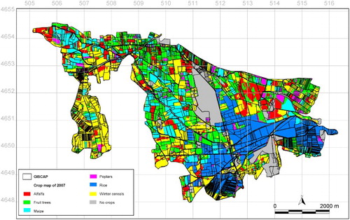
Table 1. Per-pixel confusion matrix. Global accuracy was 91.4%, calculated from the pixels correctly classified (sum of the diagonal) divided by the total number of pixels. Source: own elaboration from the hybrid classification.

	Maize	Fruit trees	Winter cereals	Alfalfa	Poplars	Rice	Total	Comission error (%)	User's accuracy (%)
Maize	298	10	0	3	0	0	311	4.2	95.8
Fruit trees	34	231	5	23	12	3	308	25.0	75.0
Winter cereals	9	3	303	3	0	0	318	4.7	95.3
Alfalfa	3	0	0	216	0	0	219	1.4	98.6
Poplars	0	22	0	0	79	4	105	24.8	75.2
Rice	13	8	0	0	0	523	544	3.9	96.1
Total	357	274	308	245	91	530	1805
Omission error (%)	16.5	15.7	1.6	11.8	13.2	1.3
Producer's accuracy (%)	83.5	84.3	98.4	88.2	86.8	98.7

In the enrichment process, applied to 3594 parcels, 1008 polygons were labeled as fruit trees, 251 as alfalfa, 479 as maize, 1140 as winter cereals, 610 as rice and 106 as poplars. A quantitative analysis of polygon enrichment by categories was applied with the objective of calculating the number of polygons with different purity intervals (Figure 2). Three different intervals were considered: up to 50% (equivalent to the parcels less likely to be correctly classified), up to 75% (more likely to be correctly classified) and up to 100% (equal to those parcels with high probability of correct classification). Poplars, fruit trees and alfalfa showed the highest percentages of parcels with low purity, with values above 10%, whereas this percentage in the case of rice was very small, as an indication of homogeneous results. In the second purity interval (up to 75%), the highest results clearly appeared in poplars and alfalfa and the lowest in rice. Finally, the best purity – up to 100% – was obtained in rice and winter cereals, in the interval for percentages above 75%. Therefore, permanent crops (deciduous trees and alfalfa) showed the worst results and winter cereals and rice the best, a coherent output compared with the confusion matrix. In the case of deciduous trees, a possible explanation is the small size of the parcels, while in the cases of winter cereals and rice the good results behave in the opposite way, as those parcels are larger.

Figure 2. Purity, by crops: percentage of polygons with up to 50%, 75% and 100% purity.

3.1. Uncertainty from purity

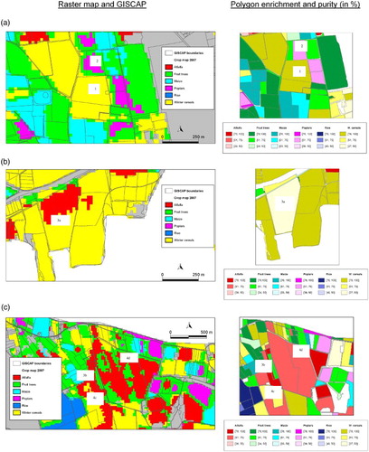
Polygon enrichment and purity allow the discrimination of four different situations (Figure 3): (i) a parcel is completely covered by just one raster category, the ideal situation because purity would be 100%; (ii) the inner part of a parcel appears clearly covered by just one raster category, but at the edges one or more different categories can appear, a situation characteristic of the border raster effect that is resolved if the border covers a small part of the parcel, producing purities below 100% but above 75%; (iii) a parcel with two clearly different raster categories, causing purities of about 50% and either a regular sprawl or an irregular sprawl; (iv) a parcel with more than two raster categories, resulting in purities either below or just above 50%, both with a regular or an irregular sprawl; regular distributions evidence a farmer's decision to occupy the parcel with two different crops. With this analysis, the user has an indirect measure of misclassification because the spatial distribution variability of classification uncertainties is known and the researcher can decide to apply a purity threshold to retain as reliable only those parcels with the highest values of purity (e.g. above 50%) and/or those with a more regular/compact distribution of the inner patches. Therefore, map usage can incorporate quantitative information about the spatial distribution of the uncertainty and even the knowledge of the uncertainty at parcel level (Rocchini et al., 2011).

Figure 3 (a). Case 1: a parcel is completely covered by just one raster category (purity = 100%). Case 2: the inner portion of a parcel appears clearly covered by just one raster category but the borders show different categories (purity above 75%). Figure 3(b). Case 3a: a parcel with two clear raster categories (purity below 50%), with a regular sprawl. Figure 3(c). Case 3b: a parcel with two clear raster categories (purity about 50%), with an irregular sprawl. Case 3c: a parcel with more than two raster categories (purity below or just above 50%), with a regular sprawl. Case 3d: a parcel with more than two raster categories but with an irregular sprawl.

4. Conclusions

The final map shows the spatial variability of classification uncertainties at parcel scale (Main Map). The three intervals of purity are shown with a graduation of color based on the Hue-Saturation-Intensity model (useful to encode uncertainty, according to Brodlie, Osorio, and Lopes (2012)), from pale, in the case of low purities, to intense, in high purities. Similar color models and uncertainty management criteria have been adopted in other geospatial work such as in Pebesma, de Jong, and Briggs (2007) or in Laskey, Wright, and da Costa (2010), both focusing on continuous variables at pixel scale, whereas this work has adopted the parcel scale. An additional improvement of our procedure, compared with other classical methods such as confusion matrices, is that all the study area is analyzed and the uncertainty related to the classification process does not remain hidden in the output map. Moreover, our spatial purity method provides information to minimize the issues related to the classification process, the border pixel effect, locations with more than one crop type, or parcel data that do not correspond to management practices.

Acknowledgements

The authors wish to thank the Ministry of Agriculture, Livestock, Fisheries, Food, and the Environment of the Catalan government for their support.

Disclosure statement

No potential conflict of interest was reported by the authors.

ORCID

Pere Serra http://orcid.org/0000-0003-1023-5586

Xavier Pons http://orcid.org/0000-0002-6924-1641

Additional information

Funding

This research has received funding from the European Community's Seventh Framework Program (FP7/2007–2013) under grant agreement n°265178, through project GEOVIQUA (QUAlity aware VIsualization for the Global Earth Observation System of Systems). Xavier Pons is the recipient of an ICREA Acadèmia Excellence in Research grant (2011–2015). This work was partially supported by the Spanish Ministry of Economy and Competitiveness and the European Regional Development Fund (ERDF) under Grant CGL2012-33927 (DinaCliVe).

References

- Aplin, P., Atkinson, P. M., & Curran, P. J. (1999). Fine spatial resolution simulated satellite sensor imagery for land cover mapping in the United Kingdom. Remote Sensing of Environment, 68, 206–216. doi: 10.1016/S0034-4257(98)00112-6
- Barbosa, P. M., Casterad, M. A., & Herrero, J. (1996). Performance of several Landsat 5 Thematic Mapper (TM) image classification methods for crop extent estimates in an irrigation district. International Journal of Remote Sensing, 17, 3665–3674. doi: 10.1080/01431169608949176
- Breckenridge, R. P., Lee, R. D., Cherry, S. J., Rope, R. C., & Dakins, M. (2008). Synthesizing old and new: Joining existing remote-sensing and GIS data to assess fire issues in sagebrush steppe ecosystem. Journal of Maps & Geography Libraries, 4, 251–268. doi: 10.1080/15420350802142421
- Brodlie, K., Osorio, R. A., & Lopes, A. (2012). A review of uncertainty in data visualization. In J. Dill, R. Earnshaw, D. Kasik, J. Vince, & P. C. Wong (Eds.), Expanding the frontiers of visual analytics and visualization (pp. 81–109). London: Springer-Verlag.
- Dean, A. M., & Smith, G. M. (2003). An evaluation of per-parcel land cover mapping using maximum likelihood class probabilities. International Journal of Remote Sensing, 24, 2905–2920. doi: 10.1080/01431160210155910
- Díaz-Delgado, J., & García-Palomares, J. C. (2014). A highly detailed land-use vector map for Madrid region based on photointerpretation. Journal of Maps, 10, 424–433. doi: 10.1080/17445647.2014.882798
- Foody, G. M. (2002). Status of land cover classification accuracy assessment. Remote Sensing of Environment, 80, 185–201. doi: 10.1016/S0034-4257(01)00295-4
- Foody, G. M. (2009). Sample size determination for image classification accuracy assessment and comparison. International Journal of Remote Sensing, 30, 5273–5291. doi: 10.1080/01431160903130937
- Iianes, J. S., Congalton, R. G., & Lunetta, R. S. (2013). Analyst variation associated with land cover image classification of Landsat ETM+ data for the assessment of coarse spatial resolution regional/global land cover products. GisScience and Remote Sensing, 50, 604–622.
- Khorram, S. (1999). Accuracy assessment of remote sensing-derived change detection (65 pages). Bethesda, MD: American Society for Photogrammetry and Remote Sensing.
- Laskey, K. B., Wright, E. J., & da Costa, P. C. G. (2010). Envisioning uncertainty in geospatial information. International Journal of Approximate Reasoning, 51, 209–223. doi: 10.1016/j.ijar.2009.05.011
- Martínez, M. (2013). Mapping spatial thematic accuracy using indicator kriging (Master's thesis). University of Tennessee. Retrieved September 26, 2014, from http://trace.tennessee.edu/uk_gradthes/2624
- Moré, G., Pons, X., & Serra, P. (2006). Application of a hybrid classifier to discriminate Mediterranean vegetation with a detailed legend and using long multitemporal series of images. 27th International Geoscience and Remote Sensing Symposium (IGARSS). IEEE Geoscience and Remote Sensing Society, Denver.
- Pebesma, E. J., de Jong, K., & Briggs, D. (2007). Interactive visualization of uncertain spatial and spatio-temporal data under different scenarios: An air quality example. International Journal of Geographical Information Science, 21, 515–527. doi: 10.1080/13658810601064009
- Peña-Barragán, J. M., Ngugi, M. K., Plant, R. E., & Six, J. (2011). Object-based crop identification using multiple vegetation indices, textual features and crop phenology. Remote Sensing of Environment, 115, 1301–1316. doi: 10.1016/j.rse.2011.01.009
- Pesquer, L., Masó, J., & Pons, X. (2000). Herramientas de análisis combinado ráster/vector en un entorno SIG. In I. Aguado & M. Gómez (Eds.), Tecnologías Geográficas para el Desarrollo Sostenible. Departamento de Geografía. Universidad de Alcalá. IX congreso del Grupo de Métodos Cuantitativos, Teledetección y SIG de la Asociación de Geógrafos Españoles (pp. 53–73). Alcalá de Henares: Universidad de Alcalá.
- Pons, X. (2006). MiraMon. Geographic information system and remote sensing software. Bellaterra, CREAF.
- Pons, X., Cristóbal, J., González, O., Riverola, A., Serra, P., Cea, C., … Velasco, E. (2012). Ten years of local water resource management: Integrating satellite remote sensing and geographical information systems. European Journal of Remote Sensing, 45, 317–332. doi: 10.5721/EuJRS20124528
- Pons, X., Moré, G., & Pesquer, L. (2010). Automatic matching of Landsat image series to high resolution orthorectified imagery. Proceedings of the ESA Living Planet Symposium, Bergen, Norway, CD-ROM edition, ESA reference document: SP-686.
- Pons, X., Pesquer, L., Cristóbal, J., & González-Guerrero, O. (2014). Automatic and improved radiometric correction of Landsat imagery using reference values from MODIS surface reflectance images. International Journal of Applied Earth Observation and Geoinformation, 33, 243–254. doi: 10.1016/j.jag.2014.06.002
- Rocchini, D., Hortal, J., Lengyel, S., Lobo, J. M., Jiménez-Valverde, A., Ricotta, C., … Chiarucci, A. (2011). Accounting for uncertainty when mapping species distributions: The need for maps of ignorance. Progress in Physical Geography, 35, 211–226. doi: 10.1177/0309133311399491
- Serra, P., Moré, G., & Pons, X. (2005). Application of a hybrid classifier to discriminate Mediterranean crops and forests. Different problems and solutions. XXII international cartographic conference, A Coruña, Spain.
- Serra, P., Moré, G., & Pons, X. (2009). Thematic accuracy consequences in cadastre land-cover enrichment from a pixel and from a polygon perspective. Photogrammetric Engineering and Remote Sensing, 75, 1441–1449. doi: 10.14358/PERS.75.12.1441
- Serra, P., &, Pons, X. (2013). Two Mediterranean irrigation communities in front of water scarcity: A comparison using satellite image time series. Journal of Arid Environments, 98, 41–51. doi: 10.1016/j.jaridenv.2013.07.011
- Serra, P., Pons, X., & Saurí, D. (2003). Post-classification change detection with data from different sensors: Some accuracy considerations. International Journal of Remote Sensing, 24, 3311–3340. doi: 10.1080/0143116021000021189
- Skokanová, P., Havlíček, M., Borovec, R., Demeka, J., Eremiášová, R., Chrudina, Z., … Svoboda, J. (2012). Development of land use and main land use change processes in the period 1836–2006: Case study in the Czech Republic. Journal of Maps, 8, 88–96. doi: 10.1080/17445647.2012.668768
- Steele, B. M., Winne, J. C., & Redmond, R. L. (1998). Estimation and mapping of misclassification probabilities for thematic land cover maps. Remote Sensing of Environment, 66, 192–202. doi: 10.1016/S0034-4257(98)00061-3
- Stehman, S. V. (2009). Sampling designs for accuracy assessment of land cover. International Journal of Remote Sensing, 30, 5243–5272. doi: 10.1080/01431160903131000
- Stehman, S. V., & Wickham, J. D. (2011). Pixels, blocks of pixels, and polygons: Choosing a spatial unit for thematic accuracy assessment. Remote Sensing of Environment, 115, 3044–3055. doi: 10.1016/j.rse.2011.06.007
- Zhan, Q., Molenaar, M., Tempfli, K., & Shi, W. (2005). Quality assessment for geo-spatial objects derived from remotely sensed data. International Journal of Remote Sensing, 26, 2953–2974. doi: 10.1080/01431160500057764