Spatiotemporal distribution of Landsat imagery of Europe using cloud cover-weighted metadata

ABSTRACT

Landsat imagery is the most frequently used remotely sensed data in many fields related to the monitoring of the Earth's surface. As Landsat satellites have gathered data since 1972, lots of valuable information has been stored and can be derived from imagery over a long time interval. Of course, due to certain factors such as weather conditions and satellite-related technical issues, data collection cannot be consistent in time and space. Cloud coverage is the most obvious condition that determines the usability of a remotely sensed satellite images. For successful results, a rich data supply is essential. To explore the data supply of a certain study area, the Landsat metadata can be checked which is usually an involved process especially for a long time interval. Therefore, the visualisation of Landsat metadata can result in a faster work flow and successful study area selection. In this paper we present a cloud cover-weighted metadata map for the area of Europe.

KEYWORDS:

• Landsat
• spatiotemporal
• data supply
• metadata
• cloud cover
• index

1. Introduction

Landsat has the longest continuity amongst medium resolution Earth observation satellite programmes with the first images being acquired in 1972. The programme covers 44 years, which is unique in detailed resolution environment monitoring. The Landsat series of satellites provides the longest temporal record of space-based surface observations and remarkably, the record is unbroken with most land locations acquired at least once per year since 1972 (Roy et al., 2014). The longest running satellite imagery acquisition enterprise has already launched eight satellites and all but one (Landsat 6) provided data successfully. Currently, two satellites are operational (Landsat 7 and Landsat 8). The most successful member of the family is the remarkable Landsat 5, which collected data for more than 29 years and is the longest operating Earth observing satellite (Belward & Skøien, 2015). Since the launch of the first satellite many studies have used Landsat imagery as the base data. In 2008, the scientific use of Landsat imagery increased to a great extent as the United States Geological Survey (USGS) released the Landsat archive (Woodcock et al., 2008). The reason Landsat data is so widely used is its longevity and the fact that it is freely available. Landsat imagery has a good metadata supply, with all imagery downloaded from the USGS archive coming with a detailed metafile. In addition anyone can extract scene metadata from the Landsat inventory through The Landsat Bulk Metadata Service (USGS) or download the entire collection of metadata. The study of metadata is an essential prerequisite for any research, because it conveys the following information about the data: the spatial coverage and temporal resolution. Based on this information, a decision can be made about the use of the data. Ideally imagery would be available for every day of the year with optimum weather conditions. However, as Landsat missions are designed to revisit the same geographical location every 16 days, and due to varying weather conditions and satellite-related events (e.g. the Scan Line Corrector (SLC) error of Landsat 7 (Zhanga, Lia, & Travisb, 2007) and the reactivation of Landsat 5 or a new satellite launch (Irons & Loveland, 2013)), certain areas and different time intervals can be quiet diverse with respect to the number of acquired cloud-free images. Kontoes and Stakenborg (1990) estimated the number of cloud-free images acquired during the Landsat mission's first 15 years (1972–1987). Their study confirms that different areas have different number of cloud-free acquisitions due to weather conditions. Armitage, Ramirez, Danson, and Ogunbadewa (2013) used the Moderate Resolution Imaging Spectrometer cloud coverage product to calculate the probabilities of cloud-free acquisition in the case of Great Britain. Their result shows that weather conditions have a huge impact on usable data acquisition. Cloud coverage is a factor that every remote sensing-based study has to deal with. To select areas for a successful investigation and to avoid lack of data due to cloud coverage, knowledge of metadata is indispensable. However, the study of raw metadata can be a complex task especially over long time intervals. Therefore, the analysis of raw metadata can lead to a faster and more efficient working process. In this study we present a metadata map which can be of great help in choosing Landsat data. Our ‘Main Map’ shows the spatial differences in the quantity of available Landsat data.

2. Methods

We used open-source software in this study with all geoprocessing and layout editing performed in QGIS 2.6. For data conversion we used the Xml to Csv Conversion Tool (https://xmltocsv.codeplex.com/) and QGIS. After data collection we transformed the geospatial data to a format usable for visualisation: the transformation corrected the values according to cloud cover before producing a final index value. This is now discussed.

2.1. Study area

Our study area includes mainland Europe and the British Isles, including all the areas located between 11° and 30° longitude and 34° and 60° north latitude. The border of the study area is defined by the natural borders of Europe, except to the North which is defined by the 60° north latitude. For areas north of 60° Landsat images multiple overlap precludes the use of our methodology. Therefore, parts of Scandinavia above 60° north latitude are not included. We used all imagery that cover land, acquired by Landsat 4–8 between 7 May 1984 and 17 September 2014.The time interval extends from the first Landsat 5 acquisition to the date of our analysis.

2.2. Data collecting

Our goal is to visualise Landsat metadata related to each scene; for this purpose the main features of our map are the Landsat scenes according to path and row. It is clear that two types of data are needed for this task. Firstly, the geometry data, which represents the actual extent of Landsat scenes, and secondly the cloud coverage data which is the attribute that can be connected to the appropriate scene. To visualise the data, we had to have the geometry in shapefile format. We used the official wrs2_descending shapefile (https://landsat.usgs.gov/tools_wrs-2_shapefile.php) provided by the USGS. Cloud coverage data can be found in the regular metadata which comes with every Landsat image. For multiple metafile (.mtl) acquisition, the USGS's Bulk Metadata Service (http://landsat.usgs.gov/consumer.php) can be used as an official tool. The metadata used in this study is downloaded through the above-mentioned service in XML format.

2.3. Data processing

The XML metadata was first converted to the CSV file using the Xml to Csv Conversion Tool before the CSV was converted to a shapefile using QGIS. The result of the conversion was an editable database related to cloud coverage. Our purpose was to determine the number of images with a given maximum cloud coverage acquired during the examined time interval for each scene. For more manageable data handling, we classified the data into cloud coverage categories as follows: ‘<1%’ (cloud free), ‘≤10%’, ‘≤20%’, ‘≤30%’, ‘≤40%’ and ‘≤50%’. In our investigation we did not account for imagery with cloud coverage over 50%, because these images are unsuitable for many applications. With a complex query, the number of available imagers was specified for each cloud coverage category and each scene. Thereafter, the number of available images was registered into the attribute table of the wrs2_descending shapefile using a spatial join vector. As the information on cloud coverage in the metadata is at the scene level, our map shows the cloud coverage probability at the scene level also. For further analysis we dealt with overlapping, which exists in longitudinal and latitudinal directions as well between Landsat scenes. Latitudinal overlaps between rows do not provide any new information as the same data are recorded for both images, so we considered those areas as part of a relevant, latitudinal neighbouring image. Longitudinal overlapping is different since two overlapping paths are travelled by the satellites with a time difference, so in this case, overlapping areas can be treated separately from neighbouring scenes. As satellites travel down from north towards the equator, the gap between their paths gets wider, hence overlaps become smaller and past the 56°N, some of them disappear, therefore areas related to only one Landsat scene appear. In the case of Europe, we find areas with and without overlapping. Longitudinal overlapping areas unequivocally have a better data supply as they are represented on two Landsat scenes and in two different paths. The values of overlapping areas have been derived from values of the two longitudinal neighbouring (not overlapping) areas as a sum of both.

2.4. Index

For more realistic metadata visualisation we created a data supply index, which represents an average probability for every pixel of a given area (i.e. how many usable images are available) using all images with ≤50% cloud coverage. The calculation considers the number of available images, with different weights according to the cloud coverage categories. The rationale for weighting is that cloud coverage decreases the usable area of images, consequently the affected images provide less data and so data loss is directly proportional to cloud coverage. The weighting is implemented as follows: <1% = 1, ≤10% = 0.9, ≤20% = 0.8, ≤30% = 0.7, ≤40% = 0.6 and ≤50% = 0.5. The equation is based on summation of values (number of images) stored in the cloud coverage categories with the proviso that each image can referenced exactly once in the final result. Because the categories are nested into each other as a cascade, the already included images have to be subtracted at each step of the summation. A different formula was applied for overlapping and single covered areas. For single covered areas we used simple weighting equation (1)(1) where N is the number of usable images for the given scene; i₀ is the number of images with cloud coverage of <1% for the given scene; i₁₀ is the number of images with cloud coverage of ≤10% for the given scene; i₂₀ is the number of images with cloud coverage of ≤20% for the given scene; i₃₀ is the number of images with cloud coverage of ≤30% for the given scene; i₄₀ is the number of images with cloud coverage of ≤40% for the given scene; and i₅₀ is the number of images with cloud coverage of ≤50% for the given scene.

For overlapping areas, in addition to the weighting, we applied a coefficient as a correction for the SLC error data loss. The correction coefficient is calculated as the number of ETM+ SLC-off images multiplied by the average data loss in percentage. As the SLC error caused data loss increases to the longitudinal edges of the images, the average data loss in the case of overlapping areas is 37.5%, and 2.5% in the case of single covered areas. Consequently, we set the data loss factor to 35% (the difference between data loss of overlapping and single covered areas), applied as a constant equation (2)(2) where i_SLC is the number of SLC error affected images for the given scene.

The index gives the result for a specified time interval (7 May 1984 to 17 September 2014 in this study). The difference in the amount of usable imagery between overlapping and single covered areas decreased compared to the case when the simple imagery number was applied, but overlapping areas still give better possibilities for studies.

2.5. Map creation

The final map was produced from the polygon layer which contains the index values as an attribute visualised with graduated colours in the quantile mode, using 10 categories according to the index value. This is underlain by a hill shade layer, derived from Shuttle Radar Topography Mission (SRTM) data to make the mountain regions easily distinguishable from low-lying areas.

3. Results

In this study we used the metadata of 136,275 Landsat imagery acquired between 7 May 1984 and 17 September 2014. We considered 86,485 images usable as these met our criteria, and have a cloud coverage ≤50%, 22,255 cloud free.

3.1. Temporal distribution

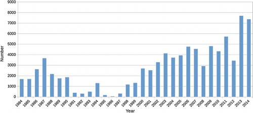
The research verified that the number of available Landsat imagery is diverse with respect to the temporal and spatial distribution. There are certain time intervals with good capabilities for scientific study (Figure 1) others have less or even close to zero likelihood, based on the number of available cloud-free images for each year. Figure 2 shows the temporal distribution of the 86,485 imagers showing that a high number of usable images do not result in a high number of cloud-free images. For example, in 2007, 36.14% of the usable images are cloud free. In contrast, in 1998 only 14.11% are cloud free. Weather conditions on the acquisition days are the key factor, which determines the possible number of cloud-free images over a time interval. Another factor is the number of possible Landsat acquisition days, which was 45–46 days annually (using two satellites). Between 1993 and 1999 only one satellite (Landsat 5) was operational as Landsat 4 had been decommissioned and the launch of Landsat 6 failed. Consequently, there is a reduction in the quantity of available images during that period. Data started to increase again after the successful launch of Landsat 7 in 1999 (Figures 1 and 2). For most studies, large amounts of cloud-free images are not essential as investigation can be still undertaken.

Figure 1. Number of cloud-free Landsat images, acquired between 7 May 1984 and 17 September 2014, available in the USGS archive.

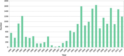
Figure 2. Number of Landsat images with a cloud cover ≤50%, acquired between 7 May 1984 and 17 September 2014, available in the USGS archive.

3.2. Spatial distribution

Spatial distribution shows the number of available images for each point of the area over the time interval. Two major parameters which have effect on the number of usable images at a certain point are weather conditions and satellite path overlap. The best areas (with more than 400 available images) are those where the number of hours of sunshine is well above the average. Consequently, poorly supplied areas are those regions where there is no satellite path overlap and the duration of sunshine is below average. The difference between areas with good and bad conditions can be large. For example, the area which is covered by the overlap of path 202 and 203 in row 33 (southern Portugal) has 265 cloud-free images while the area at path 201 and row 26 (Normandy) where there is no overlap has only 19 images with a cloud cover of <1%. Areas with good conditions such as the southern part of the Iberian Peninsula or the Carpathian Basin have much higher quantities of usable data than areas with poor conditions, such as the British Isles or much of France.

3.3. Data accuracy

For the <1% cloud coverage category, the usable imagery number assigned to certain areas is valid for each and every point of the given area, but there is increasing uncertainty as cloud coverage rises, as we do not know the exact location and shape of clouds above the area. So if there is an image with 20% of its area covered by clouds, it is only known that the 80% of its area will be usable, but the exact pixels are not known. The problem multiplies in the case of overlapping areas as the imagery number is derived from two scenes. This decreases the accuracy and reliability of the metadata map. It is important to note that images in two neighbouring satellite paths are acquired with one day difference (by different Landsat satellites), so the overlapping areas do not have a temporal overlap. For a single Landsat scene acquisition happens with an 8-day interval, whereas here there are alternating 1 and 7-day intervals. One day intervals are essential for some studies (especially for those which deal with comparison between ETM+ and OLI sensors), but irrelevant for others, and therefore these plus images do not increase the usable quantity of data in practice. Another problem is the data loss of ETM+, which mostly affects the overlapping areas.

4. Conclusions

We examined the temporal and spatial distribution of available Landsat imagery and converted the metadata to a spatially displayable database in favour of creating metadata map. During the process uncertainty was noted concerning data accuracy and usability related to growing cloud coverage, overlap issues and data loss caused by the SLC error of Landsat 7. For more realistic visualisation we created an index to represent the data supply for each area. The final metadata map may help researchers find and select the best study area quickly with an appropriate amount of Landsat imagery that can ensure success for a study.

In the near future the amount of publicly available remotely sensed satellite data will significantly increase (e.g. availability Sentinel-2 data). As the amount of data grows, it will become increasingly necessary to create a worldwide database to visualise metadata and make metadata search simpler. Our spatiotemporal distribution map of Landsat imagery for Europe is the first step.

Software

We used open-source software with data conversion, processing and layout editing performed using QGIS 2.6. Additional scripting was undertaken using GDAL.

Disclosure statement

No potential conflict of interest was reported by the authors.

References

- Armitage, R. P., Ramirez, F. A., Danson, F. M., & Ogunbadewa, E. Y. (2013). Probability of cloud-free observation conditions across Great Britain estimated using MODIS cloud mask. Remote Sensing Letters, 4(5), 427–435. doi:10.1080/2150704X.2012.744486
- Belward, A. S., & Skøien, J. O. (2015). Who launched what, when and why; trends in global land-cover observation capacity from civilian earth observation satellites. ISPRS Journal of Photogrammetry and Remote Sensing, 103, 115–128. doi:10.1016/j.isprsjprs.2014.03.009
- Irons, J. R., & Loveland, T. R. (2013). Eighth Landsat satellite becomes operational. Photogrammetric Engineering and Remote Sensing, 79(5), 398–401.
- Kontoes, C. C., & Stakenborg, J. (1990). Availability of cloud free landsat images for operational projects. The analysis of cloud cover figures over the countries of the European communities. International Journal of Remote Sensing, 11(9), 1599–1608. doi: 10.1080/01431169008955117
- Roy, D. P., Wulder, M. A., Loveland, T. R., Woodcock, C. E., Allen, R. G., Anderson, M. C., … Zhu, Z. (2014). Landsat-8: Science and product vision for terrestrial global change research. Remote Sensing of Environment, 145, 154–172. doi:10.1016/j.rse.2014.02.001
- Woodcock, C. E., Allen, R., Anderson, M., Belward, A., Bindschadler, R., Cohen, W., … Wynne, R. H. (2008). Free access to landsat imagery. Science, 320, 1011. doi: 10.1126/science.320.5879.1011a
- Zhanga, C., Lia, W., & Travisb, D. (2007). Gaps-fill of SLC-off Landsat ETM+ satellite image using a geostatistical approach. International Journal of Remote Sensing, 28(22), 5103–5122. doi:10.1080/01431160701250416