A DEM of the 2010 surface topography of Storglaciären, Sweden

ABSTRACT

During the summer of 2010 the surface elevation of Storglaciären in northern Sweden was measured using high-precision GNSS and reflectorless Total Station surveys. The DEM created from these data contain less noise than those created from orthophotographic methods over snow covered glaciers and is therefore smoother, with fewer erroneous features in the data. The principal, though not sole, intended use for the DEM is in the calculation of surface mass balance, which has influenced decisions on what constitutes a functional part of a glacier, leading to the exclusion of features such as snow aprons and perennial ice above the bergschrund. Other peripheral features have changed since the previous, aerial survey from 1999 leading to a reduction in size of approximately 0.17 km².

KEYWORDS:

• Glacier
• DEM
• mass balance
• hydrology
• modelling

1. Introduction

Storglaciären is a small (3.016 km²) valley glacier on the eastern flank of the Kebenekaise massif in northern Sweden. It is perhaps most known for having the world's longest continuous surface mass balance record, starting in 1946 and continuing to this day under the aegis of Stockholm University and the Tarfala Research Station (Holmlund & Jansson, 1999; Holmlund, Karlén, & Grudd, 1996). Approximately every 10 years a new survey of the glacier surface elevation and its perimeter is undertaken (Stockholm University, 2015). Previous surveys were performed using aerial photographs, which presents some problems when surveying a glacier. The accumulation area of a glacier is typically covered in snow or exposed firn: snow exhibits a low contrast, near featureless surface that is very difficult to map from orthophotographs. Over fresh snow there are few if any naturally occurring markers to guide parallax measurements. Of the five historical aerial photograph data sets available over Storglaciären, only one, that from 1980, is regarded as displaying high contrast (e.g. Koblet, Gärtner-Roer, Zemp, & Jansson, 2010). This is particularly problematic when determining elevation and introduces considerable errors (e.g. Andreassen, Elvehøy, & Kjøllmoen, 2002; Koblet et al., 2010). The 1999 digital elevation model (DEM) over Storglaciären, the most accurate previous data set, has positional and vertical inaccuracies on metre scales (Koblet et al., 2010). Digital stereo-photogrammetry DEMs over a Swiss glacier, constrained with 50 permanent geodetic points, were reported to have an accuracy of  m, though no accuracy assessment was demonstrated (Kropáček, Neckel, & Bauder, 2014). Analyses of DEMs from aerial photographs over a Norwegian glacier reported uncertainties on the order of 2 m (Andreassen, Kjøllmoen, Rasmussen, Melvold, & Nordli, 2012). Aerial photograph surveys as a basis for DEM generation are therefore known to introduce metre scale uncertainties where rigorous geodetic controls are absent. It was therefore decided that the 2010 survey would be performed ‘on the ground’, using global navigation satellite system (GNSS) and Total Station surveys. A kinematic GNSS rover survey is fast, simple and effective where the glacier surface can be accessed and for other parts of the glacier the relatively new tool of reflectorless distance measuring was used. This relies on essentially the same technique as Lidar, performing repeat measurements of the same location until desired precision is achieved.

The 2010 DEM is intended primarily for use in the calculation of surface mass balance within the Tarfala Research Station monitoring effort (Holmlund, 1996; Jansson & Pettersson, 2007; Stockholm University, 2015) and it is this, in combination with survey accuracy, that determines the interval between topographic surveys. In addition to this DEM a map is produced for analogue applications including planning, navigation and plotting. In most surface mass balance calculations the DEM defines the area over which point calculations are extrapolated; common extrapolation methods include elevation dependent linear functions or, as is the case for Storglaciären, ordinary kriging (Holmlund, Jansson, & Pettersson, 2005; Huss, Hock, Bauder, & Funk, 2012; Jansson & Pettersson, 2007; Kuhn, Abermann, Bacher, & Olefs, 2009). Attempts at co-kriging of surface mass balance with topography have been tried for Storglaciären but fail due to the complex distribution of elevation, slope, curvature and aspect and their relationships with mass balance components. Mass balance may also be calculated via a volume comparison, the so-called ‘geodetic method’ (Cogley, 2009; Koblet et al., 2010; Thibert & Vincent, 2009). Alternatively mass balance may be modelled using surface topography as an input parameter (Hock, 2003; Hock & Holmgren, 1996; Hulth, Hock, & Rolstad, 2009; Pellicciotti et al., 2005).

There are other uses of both the DEM and the map derived from the DEM survey. Here we distinguish between the three-dimensional (digital) DEM product and it's 2-D derivative, the map. Studies of ice dynamics on Storglaciären require up-to-date topography in order to understand the flow patterns measured (e.g. Jansson, 1996; Pohjola, 1996). Glaciohydrological studies rely on accurate topography- and surface-type distribution (i.e. the presence and extent of surface snow, firn and ice) (Dahlke, Lyon, Stedinger, Rosqvist, & Jansson, 2012; Fountain, Jacobel, Schlichting, & Jansson, 2005; Jansson, 1996; Jansson, Hock, & Schneider, 2003). Features such as glacier moulins and crevasses are also of interest for hydrological studies as well as for safety assessments but these features are transient, opening, moving and closing continuously and expressly mapping such features introduces the distinct risk of dangerously misinforming both scientists and the general public and are therefore not shown in this map. More generally, the map should be an aid to visiting researchers at the Tarfala Research Station, which through the Interact project (INTERACT, 2015) number at least 10 per year.

2. Methods

2.1. Data collection

Between the 24 July and 4 August 2010 a field survey of the surface topography and extent of Storglaciären in northern Sweden was performed using two instruments from Trimble Navigation Limited (T.N.L.): an R7 GNSS and an S6 DR series Total Station. The survey consisted of kinematic GNSS surveys of the glacier surface and perimeter where access was considered safe. Where safe access could not be gained, as well as in a few areas where extreme topography blocked satellite coverage, a reflectorless Total Station survey was performed from temporary benchmarks established using fast static GNSS surveys. The reflectorless survey measures the distance to a target and adjusts for the height of the target using the incidence angle of the transmitted beam. This facilitates remote surveys: in the case of Storglaciären, reflectorless Total Station surveys were used to map surface elevations in the crevasse fields, at the margins where access was limited by avalanche hazards and along the southern boundary of the glacier, where satellite reception was too poor to achieve a fixed solution. The total extent measured this way is at most 26% by area, the interpolation between areas measured by the different methods making an exact figure difficult to estimate. The GNSS data were post processed against reference data from the Tarfala Research Station's own base station (also a Trimble R7). This base station had previously been fixed into the SWEREF99 reference system with the aid of the SWEPOS post processing service (Lantmäteriet, 2015).

The kinematic GNSS survey has a nominal accuracy for height measurements of , which would give a maximum error of 20 mm at the antenna for those points farthest from the base station (see Trimble Navigation Limited, 2013a). To this must be added the imprecision introduced by the positioning of the antenna over the surface or detail being measured. The antenna was mounted on a pole attached to a backpack and the height above the ice surface measured at regular intervals throughout each day. The survey controller was set to record a data point every 5 seconds and as such no guarantee could be made that the surveyor's stance at the time of data collection gave the same signal height as that measured when standing still. This error is estimated to 5 mm through the combination of ice surface roughness and the influence of the gait of the surveyor. Data acquisition in this manner naturally creates anisotropic data distribution; there are many points, densely spaced, along the survey lines but between survey lines there is no data. Lines were surveyed following topographic features rather than at evenly spaced grid locations but with a maximum distance of 75 m between lines maintained where possible. This method was chosen firstly because of difficulties accessing all parts of the glacier but also because the data was to be processed to a triangulated irregular network (TIN).

Temporary benchmarks were set as required using tripod and tribrach. Surveyed with the R7 GNSS, the accuracy of the coordinates at the tribrach was (see Trimble Navigation Limited, 2013a). From this the S6 Total Station could measure distance with an accuracy of and angles to 0.15 mgon (see Trimble Navigation Limited, 2013b). This would give a maximum measurement error in height of 1.5 mm at a distance of 600 m from the instrument. These instrument errors may sum to no more than perhaps 50 mm in height and if we assume that each station remains stable for the duration of its use then the instrument itself introduces no further errors of any significance. A far greater error source is targeting, given that the Total Station was used mostly to survey inaccessible areas of the glacier. Targets were located at some distance and, in some cases, at quite oblique angles. The errors introduced here are essentially impossible to quantify and vary from data point to data point. Experience of surveying and of glaciers suggests that these errors should, in the majority of cases, be no greater than 100 mm. Much larger errors, of several metres, are relatively easy to identify and discard but errors on scales of around 1 m are difficult to detect in isolation. These can be more easily found when compared to neighbouring points and observations in the field. As each survey was processed the same day such errors were relatively easy to identify and rectify.

The total number of data points collected was 12,548 or approximately one point in every 240 m², which if evenly spaced, would be one point every 16 m. The distribution of this data is not even but rather strongly biased towards the lines covered by the survey team. Furthermore, the ablation area is covered by a higher spatial density of survey points than the accumulation area, due to the varying coverage of the two survey methods. The heterogeneity of the data distribution leads to inappropriate interpolation results; TINs acquire multiple, elongated triangles along survey lines, blocking triangulation between survey lines whilst statistical methods such as inverse distance weighting are biased towards the along line distribution of values. Therefore the data were thinned down to 2956 points, extracted along survey lines using a maximum Euclidian distance of 20 m. The TIN calculated from these data were gridded to a pixel spacing of 5 m for use with mass balance calculations; however, the nominal resolution for most of the glacier is 20 m.

2.2. When to map a glacier

The surface of a glacier is dynamic, the ice itself moves, if only slowly, on the time scale of a GNSS survey; more importantly, the snow and ice surfaces are ablating during the summer and are therefore lowering. In the ablation area this lowering is partly countered by the dynamic response of the glacier but by no means entirely so. Average ablation area surface lowering was approximately 0.15 m/day for the ablation area and  m/day for the accumulation area during the time of survey. Emergence velocities (resulting in uplift caused by ice flow regimes) in the ablation area are  m/yr for most of the ablation area, reaching an estimated 2.6 m/yr near the glacier front (Pettersson, Jansson, Huwald, & Blatter, 2007). Whilst it is not unreasonable to question the timing of the survey, especially as it required several days to perform, the ablation occurring during the survey is expected to be considerably less than the errors associated with photogrammetric aerial photograph surveys.

An ideal time for the survey, when considering the exposure of the summer surface and its stability would, in the case of Storglaciären, be sometime in mid-September. A minor consideration for this study was the availability of staff and resources at this time; at the end of the melt season but before first snow fall, the Tarfala Research Station staff would be performing mass balance surveys on several glaciers and thus not readily available for other mapping work. More importantly, the 2010 data were intended to be comparable with previous data from 1959, 1969, 1980, 1990 and 1999 (Koblet et al., 2010). These data were collected from aerial photographs which entails specific requirements such as relatively cloud free conditions and, as far as is possible, a snow free surface. The risk of snow fall in late August and early September is quite large and only a thin layer of snow is required to severely impair the possibility of using aerial photographs to map surface elevation. For these reasons the previous surveys have been performed in late July and early August and therefore the 2010 survey, whilst not dependent on the same conditions, was also performed during this period.

2.3. Identifying the perimeter

The definition of an object boundary requires clear protocols to explain subject decisions and promote reproducibility. For glaciers, decisions must be made such as when to include ice-cored moraines, ice-marginal snow bodies and other features. In the northern cirque of Storglaciären there are several perennial snow and ice fields above the bergschrund; at the front of the glacier snow cover often forms an apron. In Raup and Khalsa (2007) users are instructed to include ice above the bergschrund as avalanching from this region often contributes to glacier mass balance. The mass balance programme run by Tarfala Research Station includes this mass in its field survey of the glacier proper, indeed all avalanche mass, regardless of origin, is included if it has fallen onto the glacier. Extrapolating mass estimates from the avalanche covered areas back to their sources would introduce a large overestimation of accumulated mass. As the mass balance programme is one of the main end users of the DEM, it was deemed inappropriate to include these perennial fields into the main body of the glacier. Their extent is indicated by a red, dashed line on the map.

Whilst there was no apparent dead ice on Storglaciären there has for some time been an area of snow on the northern flank, near the front, that has had little interaction with the rest of the glacier. This snow patch is down slope of an abrupt end to the northern margin of the glacier and at first glance may appear to be the continuation of this flank. It is tempting to interpret the interruption as rock fall or other debris covering the glacier surface but this is not the case, instead this is a ridge of bedrock called a riegel. The riegel runs north–south, across the flow line of the glacier, strongly influencing glacier dynamics and in turn, topography. Below the riegel the lee effect allows for deep snow cover to build up in winter. This field has long been considered an active part of the glacier, at least in terms of mass balance. During 2010 this field seemed intact and stable, if somewhat down wasted, but by 2013 it was evident that it was no longer connected to the glacier in any meaningful way. The map is intended as a representation of the glacier in 2010 and this region is therefore kept in the map. This treatment of dead ice and marginal snow fields has been implicit in previous models of the glacier surface and will continue in future surveys, rationalising protocols to be in line with praxis.

In order to maintain consistency with other survey methods the delineation of the boundary in the field attempted to consider how a remote sensing analyst might interpret the surface and topographical clues. Despite this there is an inconsistency between the 1999 aerial photograph-based survey and the 2010 ground-based survey on the southern flank of the glacier. Here there is an area of lateral moraine that has been ice cored and is often snow covered or at least contains snow patches. In 2010 this area was judged to not be a part of the glacier and seemed to be easily distinguishable as inactive moraine, its flat form suggesting an absence of ice core. The absence of a core of ice in the moraine is the deciding factor in this case. These marginal features illustrate the dynamic nature of glaciers and the need to continuously update DEMs for mass balance calculations.

2.4. Data processing

The survey data, after processing to SWEREF99 TM for the (x, y) components and RH2000 for elevation (z), was interpolated to a surface by creating a TIN. The TIN was then sampled to a raster grid and masked to the measured perimeter of the glacier. This raster grid is the DEM for Storglaciären in 2010 as illustrated in the map associated with this article.

2.5. Other considerations

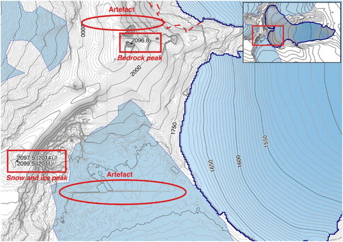
The background of the map, those areas outside Storglaciären, consists of contours derived from the Koblet et al. (2010) reanalysis of aerial photographs from 1999. The DEM produced by that work contains some linear artefacts, some of which are highlighted in Figure 1. These features seem to result from tiling at some stage of the model creation rather than representing the edges of the photographs themselves.

Figure 1. Artefacts in the orthophotograph derived DEM of 1999 (see Koblet et al., 2010). Also indicated is the elevation change in Kebnekaise's Sydtoppen.

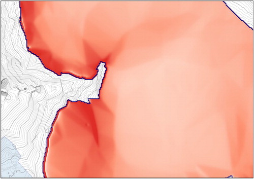
In the new, 2010 DEM other linear features may be found, but these only become evident when creating derived products such as slope. In Figure 2, a map of surface slope reveals triangular facets resulting from the TIN, which served as the base from which the final raster grid was created. These can clearly be seen in the accumulation area of the glacier and are illustrated more closely in Figure 3. The facets exist elsewhere but are more evident in those areas where field data are sparser. The TIN itself is constrained by the original survey lines and these are surveyed along perceived break lines in topography and then supplemented where possible. Therefore these facets may be considered as a simplification of the topography rather than an error, though it is an important consideration should the underlying DEM be used for modelling glacier mass balance as slope and aspect are common parameters for energy balance-type models (Hock, 2005; Hock & Holmgren, 2005). Nevertheless, much of the glacier surface is relatively smooth with a mean slope of 10° (with a minimum slope of 0.5° and a maximum of 75°). The 1999 DEM was produced from 1:30,000 scale photographs with a grid spacing of 5 m (e.g. Koblet et al., 2010). When produced this DEM was the most accurate representation of the surface of the glacier. The mean horizontal error relative to differential GNSS surveyed points was 2.74 m; vertical accuracy was assessed as ‘too low by a few metres’ (e.g. Koblet et al., 2010).

Figure 2. The surface slope of the glacier derived from the DEM. Triangular facets are found at the western margin of the glacier as a result of interpolation using a TIN.

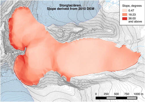
Figure 3. A close-up image of the western margin of the glacier illustrating triangular facets resulting from interpolation using a TIN.

A further feature highlighted in Figure 1 and shown on the main map is the change in elevation of Kebnekaise's Sydtoppen. This peak is officially Sweden's highest mountain top but its upper reaches consist of a snow and ice pack some 30 m thick. Both Sydtoppen and Nordtoppen, which is entirely bedrock, were surveyed using the Trimble R7 rover and base station in 2011 and a Trimble Geo7X rover in 2014. Nordtoppen remains at 2096.8 m a.s.l. whilst Sydtoppen has lowered to 2097.5 m a.s.l. by 2014, just 0.7 m higher. This trend is likely to continue and is of some interest for glaciologists, tourists and mountain safety experts alike.

3. Conclusions

A new DEM and map of Storglaciären was produced exploiting the precision available from modern in situ survey methods. Data density in the accumulation zone is much lower than for the ablation zone for both methods but for different reasons; however, as each data point in the new model is a more accurate representation of the surface it represents, the model as a whole is improved. The smoothness of the elevation data is not maintained in products derived from it. Derivatives, such as slope and curvature as well as aspect, exhibit faceting created by the initial TIN, which itself is strongly influenced by the original survey lines.

When compared with the previous DEM, derived from aerial photographs, these artefacts seem less problematic as there is considerably less noise in the data and the TIN leaves only artefacts which can be directly attributed to features of the topography. The previous data do have some advantages over the 2010 data as it covers a much larger area and does so almost instantaneously. These advantages are not insignificant, especially in glacier surveys, where the survey object experiences almost constant change. However, the majority of the errors in the older data set, particularly over steep and low contrast regions, are not repeated in the method applied to the 2010 data set and hence the 3-D accuracy of the latter product is superior.

The area calculated for Storglaciären from the 1999 DEM is 3.189 km² and the area in 2010 is 3.016 km²; however 0.110 km² of this is the moraine area on the southern side judged to no longer be part of the glacier. This leaves 0.064 km² of change, most of which stems from small differences in how high elevation, steeply sloping, snow filled gullies were interpreted.

The differences in elevation between 1999 and 2010 data sets is clearly visible in the displacement of contour lines at locations along the glacier perimeter. These are partly due to the interim 11 years during which continued down wasting of the glacier resulted in a shift of some contour lines up glacier, i.e. westward. Other differences should be interpreted as either parallax errors due to a lack of reference points or are due to orthorectification errors introduced partly by the steep terrain but also again by the paucity of available control points. The results of the mapping (see Main Map), in the form of a DEM and 2-D map, will be available to interested researchers via the Bolin Centre for Climate Research, Stockholm University (www.Bolin.su.se).

Software

Trimble Business Center was used for the post processing of GNSS data from the R7 rover unit against the base station R7 unit. Total Station data were processed to SWEREF99 TM coordinates and combined with the GNSS data using SBG Geo. GDAL was used via the Quantum GIS (QGIS) interface for the creation of the TIN, interpolation of the TIN to a raster grid and for the creation of the contour and slope data. QGIS was also used for preparation of the final map.

Acknowledgments

The work of Koblet et al. (2010) has been essential to the production of this map and I would very much like to acknowledge their contribution to this map. I would like to thank the staff of the Tarfala Research Station, particularly Raphael Jensen for his help during the field work. I would also like to thank Peter Jansson and Gunhild Rosqvist for their advice and input during this work. Ian Brown, of Stockholm University, has provided indispensable guidance during the rewriting of this manuscript.

Disclosure statement

No potential conflict of interest was reported by the author.

References

- Andreassen, L. M., Elvehøy, H., & Kjøllmoen, B. (2002). Using aerial photography to study glacier changes in Norway. Annals of Glaciology, 34, 343–348. doi: 10.3189/172756402781817626
- Andreassen, L. M., Kjøllmoen, B., Rasmussen, A., Melvold, K., & Nordli, Ø. (2012). Langfjordjøkelen, a rapidly shrinking glacier in northern Norway. Journal of Glaciology, 58, 581–593. doi: 10.3189/2012JoG11J014
- Cogley, J. G. (2009). Geodetic and direct mass balance measurements: comparison and joint analysis. Annals of Glaciology, 50, 96–100. doi: 10.3189/172756409787769744
- Dahlke, H. E., Lyon, S. W., Stedinger, J. R., Rosqvist, G., & Jansson, P. (2012). Contrasting trends in floods for two sub-arctic catchments in northern Sweden – Does glacier presence matter? Hydrology and Earth System Sciences, 16, 2123–2141. doi:10.5194/hess-16-2123-2012. Retrieved from http://www.hydrol-earth-syst-sci.net/16/2123/2012/
- Fountain, A. G., Jacobel, R. W., Schlichting, R., & Jansson, P. (2005). Fractures as the main pathways of water flow in temperate glaciers. Nature, 433, 618–621. doi:10.1038/nature03296. Retrieved from http://dx.doi.org/10.1038/nature03296
- Hock, R. (2003). Temperature index melt modelling in mountain areas. Journal of Hydrology, 282, 104–115. doi: 10.1016/S0022-1694(03)00257-9
- Hock, R. (2005). Glacier melt: a review of processes and their modelling. Progress in Physical Geography, 29, 362–391. doi:10.1191/0309133305pp453ra
- Hock, R., & Holmgren, B. (1996). Some aspects of energy balance and ablation of storglaciären, Northern Sweden. Geografiska Annaler, Series A, Physical Geography, 78, 121–131. Retrieved from http://www.jstor.org/stable/520974 doi: 10.2307/520974
- Hock, R., & Holmgren, B. (2005). A distributed surface energy-balance model for complex topography and its application to Storglaciären, Sweden. Journal of Glaciology, 51, 25–36. doi:10.3189/172756505781829566
- Holmlund, P. (1996). Maps of Storglaciären and their use in glacier monitoring studies. Geografiska Annaler Series A-Physical Geography, 78, 193–196. doi:10.2307/520981
- Holmlund, P., & Jansson, P. (1999). The Tarfala mass balance programme. Geografiska Annaler Series A – Physical Geography, 81, 621–631. doi: 10.1111/j.0435-3676.1999.00090.x
- Holmlund, P., Jansson, P., & Pettersson, R. (2005). A re-analysis of the 58 year mass-balance record of Storglaciaren, Sweden. Annals of Glaciology, 42, 389–394. doi: 10.3189/172756405781812547
- Holmlund, P., Karlén, W., & Grudd, H. (1996). Fifty years of mass balance and glacier front observations at the Tarfala research station. Geografiska Annaler Series A – Physical Geography, 78, 105–114. doi:10.2307/520972
- Hulth, J., Hock, R. M., & Rolstad, C. (2009). An enhanced distributed temperature-index melt model including radiosonde data and solar radiation. American Geophysical Union, 31, 0457.
- Huss, M., Hock, R., Bauder, A., & Funk, M. (2012). Conventional versus reference-surface mass balance. Journal of Glaciology, 38, 1–9.
- Interact (2015). INTERACT. Retrieved from http://www.eu-interact.org/
- Jansson, P. (1996). Dynamics and hydrology of a small polythermal valley glacier. Geografiska Annaler Series A – Physical Geography, 78, 171–180. doi: 10.2307/520979
- Jansson, P., Hock, R., & Schneider, T. (2003). The concept of glacier storage: a review. Journal of Hydrology, 282, 116–129. doi: 10.1016/S0022-1694(03)00258-0
- Jansson, P., & Pettersson, R. (2007). Spatial and temporal characteristics of a long mass balance record, Storglaciären, Sweden. Arctic, Antarctic, and Alpine Research, 39, 432–437. doi:10.1657/1523-0430(06-041)[JANSSON]2.0.CO;2
- Koblet, T., Gärtner-roer, I., Zemp, M., & Jansson, P. (2010). Reanalysis of multi-temporal aerial images of Storglaciären, Sweden (1959–99)–Part 1: Determination of length, area, and volume changes. The Cryosphere. doi:10.5194/tc-4-333-2010
- Kropáček, J., Neckel, N., & Bauder, A. (2014). Estimation of Mass Balance of the Grosser Aletschgletscher, Swiss Alps, from ICESat Laser Altimetry Data and Digital Elevation Models. Remote Sensing, 6, 5614–5632. doi: 10.3390/rs6065614
- Kuhn, M., Abermann, J., Bacher, M., & Olefs, M. (2009). The transfer of mass-balance profiles to unmeasured glaciers. Annals of Glaciology, 50, 185–190. doi: 10.3189/172756409787769618
- Lantmäteriet (2015). SWEPOS. Retrieved from https://swepos.lantmateriet.se/
- Pellicciotti, F., Brock, B., Strasser, U., Burlando, P., Funk, M., & Corripio, J. (2005). An enhanced temperature-index glacier melt model including the shortwave radiation balance: Development and testing for Haut Glacier d'Arolla, Switzerland. Journal of Glaciology, 51, 573–587. doi: 10.3189/172756505781829124
- Pettersson, R., Jansson, P., Huwald, H., & Blatter, H. (2007). Spatial pattern and stability of the cold surface layer of Storglaciaren, Sweden. Journal of Glaciology, 53, 99–109. doi: 10.3189/172756507781833974
- Pohjola, V. A. (1996). Simulation of particle paths and deformation of ice structures along a flow-line on storglaciären, Sweden. Geografiska Annaler. Series A, Physical Geography, 78, 181–192. Retrieved from http://www.jstor.org/stable/520980 doi: 10.2307/520980
- Raup, B. H., & Khalsa, S. (2007). GLIMS analysis tutorial, GLIMS. Retrieved from http://www.glims.org/MapsAndDocs/assets/GLIMS_Analysis_Tutorial_a4.pdf
- Stockholm University (2015). Bolin Centre Database, Tarfala Data. Retrieved from http://bolin.su.se/data/tarfala/
- Thibert, E., & Vincent, C. (2009). Best possible estimation of mass balance combining glaciological and geodetic methods. Annals of Glaciology, 50, 112–118. doi: 10.3189/172756409787769546
- Trimble Navigation Limited (2013a). TRIMBLE R7 GNSS SYSTEM - DATA SHEET, Retrieved from http://trl.trimble.com/docushare/dsweb/Get/Document-365914/022543-367D_R7GNSS_DS_0213_LR.pdf
- Trimble Navigation Limited (2013b). TRIMBLE S6 TOTAL STATION - DATA SHEET, Retrieved from http://trl.trimble.com/docushare/dsweb/Get/Document-208580/022543-098L_TrimbleS6_DS_0613_LR.pdf