Late Holocene evolution of glaciers in the southeastern Alps

ABSTRACT

The Julian Alps (in the southeastern European Alps, Italy and Slovenia) represent an important case study area for the study of small and very small maritime glaciers. High mean annual precipitation results in great snow accumulation during the winter, permitting the presence of ice bodies with the lowest Equilibrium Line Altitudes in the Alps. During the Little Ice Age (LIA) 19 small glaciers (<1 km²) existed, covering a total area of 2.4 km². By 2012, the glacierized area had shrunk by 84% and only isolated glacierets and ice patches survived, each having a total area less than 0.5 km². We present here a geomorphological and palaeoglaciological map of 8 sections of the Julian Alps related to the late Holocene distribution of glaciers, at a scale of 1:6000. Glacier topography during the LIA maximum was reconstructed on the basis of well-expressed geomorphological features together with historical archive data. The present-day distribution of ice bodies was inferred from orthophotos and 1 m resolution digital terrain models derived from airborne laser scanning. The past and present areal extent and surface morphology of glaciers permits calculation of volume loss since the LIA, which is estimated at 96%.

KEYWORDS:

• Maritime glaciers
• Little Ice Age
• volume-area scaling
• Holocene
• Alps

1. Introduction

Within international climate monitoring programmes, mountain glaciers are broadly acknowledged as excellent climate indicators (Haeberli, Hoelzle, Paul, & Zemp, 2007), and their evolution is recognized as one of the best indicators of climate change (Diolaiuti, Bocchiola, Vagliasindi, D’Agata, & Smiraglia, 2012; Lucchesi, Fioraso, Bertotto, & Chiarle, 2014). Glacier mass balance varies with altitude, regional position, aspect, gradient, glacier size, glacier type and detailed topographic position (Evans, 2006). Glaciers are also very sensitive indicators of changes in the main climatological parameters, mainly mean annual and summer air temperature (MAAT), and precipitation (MAP) (Chinn, Winkler, Salinger, & Haakensen, 2005). Since the end of the Little Ice Age (LIA, about 1865) they drastically reduced in size over the Alps by about 50% until 2000 (Painter et al., 2013; Zemp, Paul, Hoelzle, & Haeberli, 2008). It has been argued that larger glaciers retreated at a slower rate than smaller ones, the latter showing high variability in areal changes. Nevertheless, recently it has been shown how the smallest size glaciers (area <0.01 km²) lying in areas with higher accumulation and mass turnover, generally show a lower sensitivity to climate fluctuations then previously supposed. In recent decades some show stability, while their counterparts located in drier, continental settings undergo continuous shrinkage (Colucci et al., 2015; Colucci & Guglielmin, 2015; Scotti, Brardinoni, & Crosta, 2014).

Observations of the geometrical evolution of glaciers in the Julian Alps (Figure 4) started in 1880 in the Canin group, while on Montasio glacier the first survey was performed in 1921 (Desio, 1927). Glaciological surveys on Triglav glacier began later, in 1946. Nevertheless, except for Triglav, only distances from fixed benchmarks were measured and reported, while area change is generally poorly known. The maps of Canin glacier drawn by Giacomo Savorgnan di Brazzà in 1880 and by Olinto Marinelli in 1909 (Figure 1; Desio, 1927) are the best existing documentation of glacier extent in the Julian Alps at the end of the LIA. Observations carried on for the entire twentieth century but were generally restricted to length measurements from fixed benchmarks. Only recently, more detailed investigations were performed using geophysical and geodetic techniques, which allowed better characterization of the glacial remnants of the southeastern Alps, as well as a volume estimation in some case studies (Carturan et al., 2013; Colucci et al., 2015). In the Julian Alps at present 23 ice bodies cover a total area of 0.358 km², while at the LIA maximum 2.350 km² were covered by small glaciers (Colucci, 2016). Glacier reduction was particularly effective in the Canin and Triglav sectors owing to topoclimatic characteristics (Figure 2), while avalanche feeding, karstic topography and the damming effect of pronival ramparts and moraines at the snout of the glaciers exerted a geomorphological control on the evolution of the majority of ice masses in the southeastern Alps (Figure 3). For this reason, and because of higher winter precipitation observed here in the last decade, they seem to be resilient to recent climate warming instead of rapidly disappearing as might be expected (Colucci, 2016). Volume change estimations were missing, until several recent evaluations for Canin Eastern Glacieret, Triglav and Montasio (Carturan et al., 2013; Colucci et al., 2015; Del Gobbo, Colucci, Forte, Triglav, & Zorn, 2015). Despite their small size, it has been shown that these glaciers may occupy a significant fraction of ice volume at regional scale, making the production of detailed inventories important, even for glaciers down to 0.01 km² or smaller, in order to keep errors below ± 10% (Bahr & Radić, 2012; Pfeffer et al., 2014).

Figure 1. (a) The map of Raccolana Valley drawn by Giacomo Savorgnan di Brazzà in 1880; in (b) a detail of Canin glaciers and in (c) the map of Canin glaciers in 1908 produced by Olinto Marinelli, using terrestrial photogrammetric measurements.

Figure 2. (a) Photo of Canin Eastern glacier made in 1948 by Dino di Colbertaldo, and (b) in 2012.

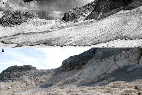
Figure 3. (a) Aerial view of Montasio West glacier in 1948, and (b) in 2011 (Service Information System and e-government, Region Friuli Venezia Giulia). Debris cover in the lower part of the glacier (upper part of the pictures) is clearly visible in 2011, while area change between 1948 and 2011 appears not particularly significant.

Therefore, the main goals of this paper are: (1) to estimate the volume of each glacier of the Julian Alps during the LIA from geomorphological evidence, (2) to quantify the volume loss since the LIA, until 2012 and (3) to present a map of late Holocene glacier extent in the LIA and in 2012, including the main geomorphological features. The LIA and 2012 glacier extent maps were produced as part of more detailed research interpreting the geomorphic control exerted by frontal ridges to small avalanche-fed glaciers (Colucci, 2016). The recent production of the extremely detailed topography of Slovenia, using light detection and ranging (LiDAR) data, was a further motivation to improve the accuracy of the inventory of glacial features in this alpine sector over the entire study area. Moreover, no estimates of the total area affected by glaciation during the LIA were reported for this alpine sector, until now.

2. Study area

The carbonate massifs of the Julian Alps extend west-east across the Italian-Slovenian border (Figure 4) and occupy 1853 km² of the southeastern Alps. Mount Triglav (2864 m; H in Figure 4) is the highest peak. The landscape of this alpine sector is largely characterized by glaciokarst (Žebre & Stepišnik, 2015) and several ice-caves are reported in the area mainly concentrated between 1500 and 2200 m with a median elevation of 1871 m (Colucci, Fontana, Forte, Potleca, & Guglielmin, 2016). Mount Canin (2587 m; C in Figure 4) forms the drainage divide between the Adriatic Sea and the Black Sea. The climatology of the Canin area for 1981–2010 has recently been reconstructed at 2200 m by Colucci and Guglielmin (2015). MAP is estimated at 3335 mm water equivalent (w.e.), while MAAT is 1.1 ± 0.6°C. Over the same period, MAAT measured at the Kredarica observatory (2514 m asl; N 46° 23′, E 13° 51′) of Mount Triglav was −1.0 ± 0.6°C and MAP was 2071 mm w.e.

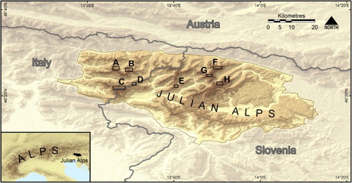
Figure 4. Location of the Julian Alps. Studied sites are marked with A, B, C, D, E, F, G and H. Base topography: ASTER GDEM (http://gdem.ersdac.jspacesystems.or.jp/).

3. Methods

The Main Map shows several geomorphological and environmental elements, but the main subject consists of glaciers, glacierets and ice patches. Seven out of the 14 detected present-day ice bodies in the Italian Julian Alps are recorded in The New Italian Glacier Inventory (Smiraglia & Diolaiuti, 2015; Smiraglia et al., 2015) and classified as glacierets and mountain glaciers. The same number of ice bodies in the entire Julian Alps is recorded in the World Glacier Inventory (https://nsidc.org/data/docs/noaa/g01130_glacier_inventory/), including only those glacierets from the Italian part of this mountain sector. The extent and geometry of former ice bodies are reconstructed mainly on the basis of geomorphological evidence, but also by using old photos and old maps. Assuming that the most extensive limit of glacial deposits belongs to the LIA, we recognized morphological evidence for ten glaciers which have not previously been reported on glaciological maps (Table 3).

3.1. Topographic base

The topographic base of the maps A, B, C, D, E, F, G and H at a scale of 1:6000 (see Main Map) is from a 1 m resolution digital terrain model (DTM), portrayed with a background shaded relief map and 25 m contour intervals. The DTM was derived from airborne laser scanning data. The Italian side of the Julian Alps was scanned on 13 September 2006 using an Optech ALTM 3033 LiDAR system. The minimum point density of this LiDAR data is 4 points per m², and the relative horizontal and vertical accuracies are better than 1 and 0.3 m respectively (Civil Defense of Friuli Venezia Giulia, 2006). Area b37, comprising all the Slovenian Julian Alps, was surveyed between 4 July 2014 and 13 January 2015 using a RIEGL LMS-Q780 scanner, producing LiDAR data with a point density from 2 to 5 per m², and relative horizontal and vertical accuracies 0.30 and 0.15 m respectively (http://gis.arso.gov.si/evode/profile.aspx?id=atlas_voda_Lidar@Arso; Geodetic Institute of Slovenia, 2015). The maps of the Italian Julian Alps (A, B, C, D) are presented in Monte Mario Italy 2 coordinate system, while the maps for the Slovenian side (E, F, G, H) use the D96 Slovenia coordinate system. The base layer of the study area map (see Main Map) is a 30 m resolution ASTER Global Digital Elevation Model (ASTER GDEM) in a World Geodetic System 1984 (WGS84) (http://gdem.ersdac.jspacesystems.or.jp/) with 20 m vertical and 30 m horizontal data accuracy (http://www.viewfinderpanoramas.org/GDEM/GDEM-README.pdf).

3.2. Data collection

Fieldwork, analysis of high resolution DTMs, orthophotos, Google Earth and Bing images as well as old pictures and maps were used in collecting the data for the map production. Fieldwork was carried out between 2011 and 2014 and included geomorphological mapping of moraines, debris flows and trimlines. Ice body boundaries in 2012 were extracted from Google Earth and Bing images for the Slovenian Julian Alps and from high resolution orthophotos for the Italian side (Service Information System and e-government, Region Friuli Venezia Giulia). Recent ice body boundaries were also compared to the glaciological, geodetic and ground penetrating radar (GPR) data performed on some of the glacierets (Carturan et al., 2013; Colucci et al., 2015). The extent of glaciers during the LIA was estimated on the basis of well-preserved frontal and lateral moraines, trimlines and by interpreting old pictures and old maps (Marinelli, 1909; Šifrer, 1963).

3.3. Geomorphological features

Landforms (morainic ridges, debris flows) were drawn on the basis of geomorphological mapping conducted in the field, and the analysis of LiDAR data, aerial photographs, archival pictures, old maps and orthophotos. The margins of former ice bodies were easily identified owing to well-preserved frontal and lateral moraines and pronival ramparts. Recognition of the upper headwall limit of ice during the LIA maximum was possible from the identification of trimlines, easily recognizable from the difference in bedrock colour. The most external system of frontal morainic ridges of Ursic, Montasio West, Canin and Triglav glaciers were attributed to the LIA maximum on the basis of the existing archival pictures dating back to the late 1800s and the early 1900s, and from the existing literature. Starting from this assumption a LIA age was also inferred for the other ice bodies. This was done taking into consideration the degree of landform preservation, the widespread lack of soil development (which suggests recent surface exposure) and their altitude in relation to the regional LIA-equilibrium line altitude (ELA) recently reconstructed by Colucci (2016) in the area.

3.4. Reconstruction of glacier topography

The former ice margins were delineated following the crests of the well-preserved frontal and lateral moraines, and evident trimlines. The LIA glacier surfaces were reconstructed based on the general morphology of present-day glaciers (Pellitero et al., 2015), having contours slightly concave up-glacier and convex near the snout (Carr, Lukas, & Mills, 2010; Porter, 1975). Ice surface contour lines were drawn at 25 m equidistance. The final DTM of each LIA glacier surface was interpolated using the Topo to Raster tool in ArcGIS.

3.5. Ice thickness calculation

The loss of ice thickness since the LIA was estimated using the Spatial Analyst Tools – Math – Minus by subtracting the DTM of recent surface topography from that of reconstructed LIA glacier surfaces. Correction of the loss of ice thickness for the Slovenian glaciers was necessary, since a lot of fresh snow was present in the examined area in the summer of 2014 (Figure 5(b); Table 1), when the airborne laser scanning for this part was performed; in contrast the Italian side was scanned in autumn 2006 (Figure 5(a)), at the end of the ablation season when no snow or just scattered fresh snow remained on the surface. Therefore, the two DTMs derived from LiDAR data in the Canin area were compared in order to estimate the mean thickness of snow cover in 2014 (on the surface of former LIA glaciers) (Figure 5(c)). Subtracting the DTM of 2006 from that of 2014, a mean snow thickness of 4.20 ± 3.98 m was calculated. This value was then added to the already calculated LIA ice thickness of Slovenian glaciers using Spatial Analyst Tools – Math – Plus. Errors in the elevation difference of the two DTMs were extrapolated from surrounding bedrock, which is assumed to have a constant elevation (Rolstad, Haug, & Denby, 2009). A mean bedrock elevation error of 0.26 ± 0.31 m was found.

Figure 5. Shaded relief of the Canin area on 13 September 2006 (a), in mid-August 2014 (b) and difference in snow cover between a and b (c). Base topography of map a: LiDAR data Italy 2006 (Civil Defense of Friuli Venezia Giulia, 2006). Base topography of maps b and d: LiDAR data Slovenia 2014–2015 (http://gis.arso.gov.si/evode/profile.aspx?id=atlas_voda_Lidar@Arso).

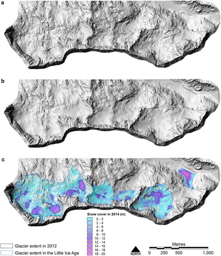
Table 1. 2014 snow cover thickness in mid-July over Canin glaciers.

ID	Name	Mean (m)	Max (m)	Min (m)	Std dev. (m)
J1	Canin West 1	8.66	14.7	0	2.87
J2	Canin West 2	11.56	16.04	0.11	1.96
J3	Canin East	11.67	16.19	2.02	3.03
J7	Prestreljenik	10.72	16.88	4.33	1.88
J8	Prevala	15.48	19.49	8.61	1.88

3.6. 2012 and LIA volume calculation

2012 and LIA glacier volumes were calculated using an empirical volume–area relation widely applied in glacier inventories and water resource estimation based on data from 144 mountain glaciers using Equation (1) from Bahr, Meier, and Peckham (1997) and Bahr, Pfeffer, and Kaser (2015) where S represents the glacier surface.(1)

The 2012 volume has then been added to the estimated volume loss calculated from the DTMs in order to achieve the best estimation of LIA glacier volumes (Table 4). To compare the results, volumes obtained through Equation (1) were plotted using data presented in Table 4 considering glacier surfaces at the LIA maximum.

3.7. Topographic names

Topographic names were obtained from topographic maps Tabacco 1:25,000 Canin – Val Resia, Parco Naturale Prealpi Giulie (‘Carta topografica per escursionisti 1:25,000. 027, Canin – Val Resia, Parco Naturale Prealpi Giulie,’ 2006) for the Italian side; and topographic maps 1:25,000 Log pod Mangartom (‘Državna topografska karta Republike Slovenije 1:25,000. 039, Log pod Mangartom,’ 1998), Breginj (‘Državna topografska karta Republike Slovenije 1:25,000. 064, Breginj,’ 1998), Kranjska Gora (‘Državna topografska karta Republike Slovenije 1:25,000. 041, Kranjska Gora,’ 1998) and Soča (‘Državna topografska karta Republike Slovenije 1:25,000. 066, Soča,’ 1995) for the Slovenian side. Both Slovenian and Italian toponyms are used for the summits situated on the border.

4. Results

The 23 permanent ice bodies mapped in the Julian Alps in 2012 covered an area of 0.383 km² (Table 2), while during the LIA maximum the glacierized area extended for 2.367 km² (Table 3). In some cases a group of ice patches has been considered a single ice body. This is the case of J1, J2, J3, J5, J6, J7, J9, J16, J20. This choice is based on the following motivations: (1) there is one main ice body and a number of minor ice patches in close proximity (e.g. J1, J2, J3, J6, J7, J9) 2) and (2) there are a number of ice patches having comparable sizes (e.g. J5, J19, J20). We recalculated and compared the volumes presented in Table 4 by using the volume-area scaling of Equation (1). Results are shown on the scatter plot (Figure 6(a)) where volumes calculated using equation 1 are presented using a logarithmic scale. As already highlighted by Bahr et al. (2015), the volume–area relationship might fail at small or large glacier sizes that fall outside their observed data (>0.1 km² and <1000 km²). In this case study it seems to underestimate the more realistic volume reconstructed from geomorphological evidence and the very high correlation (R = 0.99 and slope 1.17) is probably due to the highly skewed distribution where the two largest glaciers control slope and correlation. Therefore, we used a power-low relationship in order to infer a new volume-area scaling The results shown in Figure 6(b) with a linear trend on a log–log plot suggest a different volume–area scaling for small and very small glaciers (area <1.0 km²) down to ice patches of 0.01 km², as presented in Equation (2).(2)

Figure 6. (a) Scatter plot of LIA glacier volumes (DTM volume estimation vs. volume-area scaling volume calculation) for all the LIA glaciers in the Julian Alps and, (b) considering only the smallest size glaciers having an area < 0.1 km².

Table 2. Area of glaciers, glacierets and ice patches in 2012.

ID	Name	Area (km^2)
J1	Canin West 1	0.033
J2	Canin West 2	0.024
J3	Canin East	0.024
J4	Vasto	0.001
J5	Ursic	0.005
J6	Torre Gilberti	0.004
J7	Prestreljenik	0.024
J8	Prevala	0.013
J9	Cergnala	0.012
J10	Montasio West	0.071
J11	Montasio East	0.038
J12	Montasio Minor	0.004
J13	Studence	0.008
J14	Carnizza – Riofreddo	0.019
J15	Bavški Grintavec	0.022
J16	Zeleni sneg – Triglav	0.008
J17	Triglav minor	0.004
J18	Krnica	0.029
J19	Ponca North	0.006
J20	Ponca East	0.019
J21	Low Oltar	0.003
J22	High Oltar	0.012
J23	Dovški križ	0.002
	SUM	0.383

Table 3. Area of glaciers at the LIA maximum.

ID	Name	Area (km^2)
JL1	Canin	0.678
JL2	Ursic	0.180
JL3	Prestreljenik	0.259
JL4	Prevala	0 . 051
JL5	Cergnala	0 . 125
JL6	Montasio West	0.100
JL7	Montasio East	0.063
JL8	Montasio Minor	0.008
JL9	Studence	0 . 020
JL10	Carnizza – Riofreddo	0 . 061
JL11	Bavški Grintavec	0.058
JL12	Zeleni sneg – Triglav	0.442
JL13	Krnica	0.063
JL14	Ponca North	0 . 022
JL15	Ponca East	0 . 068
JL16	Low Oltar	0 . 020
JL17	High Oltar	0 . 042
JL18	Dovški križ	0 . 083
JL19	Kredarica	0.025
	SUM	2.367

Note: In bold ice bodies previously unreported.

Table 4. Average thickness of glaciers during the LIA on the basis of present topographic surface, loss of glacier volume since the LIA, 2012 calculated volume from Bahr et al. (1997) and Bahr et al. (2015), and LIA total volume calculated from geomorphological evidence and topography reconstruction.

ID	Name	Average thickness (km)	Volume loss (km^310^−3)	2012 Volume (km^310^−3)	LIA Volume (km^3 10^−3)
JL1	Canin	0.041	27.89	0.137	28.03
JL2	Ursic	0.015	2.70	0.029	2.73
JL3	Prestreljenik	0.019	4.90	0.147	5.05
JL4	Prevala	0.010	0.50	0.073	0.57
JL5	Cergnala	0.016	2.01	0.065	2.07
JL6	Montasio West	0.029	2.90	0.822	3.72
JL7	Montasio East	0.021	1.30	0.351	1.65
JL8	Montasio Minor	0.018	0.09	0.016	0.11
JL9	Studence	0.016	0.30	0.042	0.34
JL10	Carnizza – Riofreddo	0.017	0.99	0.137	1.13
JL11	Bavški Grintavec	0.032	1.90	0.157	2.06
JL12	Zeleni sneg – Triglav	0.031	13.80	0.029	13.83
JL13	Krnica	0.027	1.70	0.243	1.94
JL14	Ponca North	0.017	0.40	0.042	0.44
JL15	Ponca East	0.018	1.20	0.232	1.43
JL16	Low Oltar	0.011	0.20	0.042	0.24
JL17	High Oltar	0.019	0.80	0.099	0.90
JL18	Dovški križ	0.023	1.90	0.011	1.91
JL19	Kredarica	0.017	0.40	0.002	0.40
	SUM		65.88	2.68	68.55

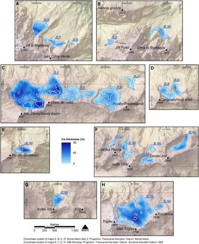
Thickness evaluation on the basis of the DTM reconstruction (Figure 7) shows maximum LIA values between 80 and 90 m in Canin, Bavški Grintavec and Triglav glaciers. Canin glacier had the maximum average thickness (41 m, Table 4) and the largest volume (0.0279 km³), approximately double that of Triglav glacier, although its area was more or less 65% of Canin. The LIA average ice thickness was equal to 29 m, while in 2012 it is calculated as 7 m. This value is reasonable if compared to that found in more detailed volume evaluation recently performed by using GPR over the Montasio glacier (average thickness ∼15 m (Carturan et al., 2013)) and the Canin east (average thickness ∼12 m (Colucci et al., 2015)) which at present represents the largest-size ice bodies in the area. Overall, we estimate the post-LIA loss in volume at 96%. Montasio East showed the lowest volume reduction of about 21%, together with Montasio West (22%). Canin and Triglav have reduced dramatically in volume and lost respectively 99.5% and 99.8% of their volume since the LIA, which is in accordance with many alpine glaciers. In 2012, their snouts were hundreds of metres from their frontal moraine ridges. This is not the case for Montasio West and East, Prevala and other ice patches still in contact with their frontal moraines or pronival ramparts. Their damming effect allows significant avalanche-snow accumulation to multiply the winter snow input several-fold, and to better preserve the ice bodies from the hotter and longer summers of recent decades (Colucci, 2016). This geomorphic control on small glaciers and ice patches of the Julian Alps is particularly evident if we consider the area response to post-LIA climate warming. The widespread mass balance decrease (excluding avalanches) observed in the last century was not followed by an equivalent area decrease. This is clearly evident in some of the smallest glaciers and ice patches of the Julian Alps. This differential behaviour seems to be characteristic of other maritime areas of the world. For example in the southern Canadian Cordillera and in British Columbia the smallest size glaciers (area < 0.4 km²) have shown no considerable changes in area between the 1950s and early 2000s due to local factors that are able to significantly decrease their sensitivity to climate change (DeBeer & Sharp, 2007, 2009). Scotti et al. (2014) presented similar evidence from the central-western Alps, in the Orobie Mountains where maritime glaciers retreated more slowly compared to glaciers in the more continental environments. Well-developed frontal moraine systems and pronival ramparts are portrayed on the Main Map. The distance between the ridge crests and the talus foot upslope is often > 30–70 m, which was considered by Ballantyne and Benn (1994) as a threshold condition for a small firn body to start moving. This suggests a coupled mechanism in the growth of such ridges, partly due to rotational creep of the ice patch and by gravitational debris supply across the topographic surface of the ice body. In some cases we observed and mapped breach-lobe moraines, typical features of glaciers with low dynamics growing more in thickness than in area (e.g. Žebre & Stepišnik, 2015). The best example was observed over the Ursic frontal moraine (Main Map, section C). The presence of two or more sub-parallel and juxtaposed frontal moraine ridges is very common in the Julian Alps, testifying to different phases, which helped the chronology reconstructions of different advances. This is especially the case for Prevala, Canin, Prestreljenik, Montasio and Krnica, allowing recognition of the 1910–1920 glacier advance observed by Desio (1927) in the Canin area and reported by Gams (1994) for Triglav. Well-preserved fluted moraines are reported on the western portion of the Canin glacier area, indicating higher dynamics, likely controlled by topography. The occurrence of heavy rainfall and debris flows mainly during summer and autumn is another important process in the destructive evolution of the ramparts and moraines. Debris flows are also shown on the Main Map, showing how in a few cases entire portions of the frontal ridges have been completely removed and washed out down valley during major rainfall events. In the Ponca North avalanche-fed ice patch, sediments are transported up to 500 m downhill from the wide apex of the ice patch in its central part, where a bergschrund was observed in 2012. Matthews, Shakesby, Owen, and Vater (2011) reported that the specific topography of sites and the balance between destructive and constructive processes led to the formation and preservation of pronival ramparts in a maritime area of Norway; the same was observed also in the Julian Alps.

Figure 7. Estimation of the loss of ice thickness since the LIA. IDs of glaciers during the LIA are written in white-blue colour. White polygons mark recent extent of glacial bodies. Base topography of maps A, B, C and D: LiDAR data Italy 2006 (Civil Defense of Friuli Venezia Giulia, 2006). Base topography of maps E, F, G and H: LiDAR data Slovenia 2014–2015 (http://gis.arso.gov.si/evode/profile.aspx?id=atlas_voda_Lidar@Arso).

5. Conclusions

A complete characterization of ice bodies in the southeastern European Alps (Julian Alps) has been produced for the first time. Detailed geomorphological mapping and LiDAR surveys permitted the evaluation of the evolution of surface topography, thickness and the volume of glaciers in the late Holocene, that is, at present (2012) and during the LIA maximum. The volume of small glaciers in the Julian Alps decreased drastically, by about 96%. Today only isolated glacierets and ice patches persist, having avalanche feeding and low dynamics. High precipitation permits their existence at the lowest altitude in the Alps.

Software

All stages of the map production, which included georeferencing, digitizing, DTM analyses, data collection and final layout, were carried out using ESRI ArcGis 10.3.1.

Acknowledgements

Valuable help during the fieldwork activities was given by the Ente Parco Naturale Regionale delle Prealpi Giulie. We also thank Ian S. Evans, Matteo Spagnolo and Thomas Pingel for their useful reviews which improved the paper, as well as the editor.

Disclosure statement

No potential conflict of interest was reported by the authors.

Additional information

Funding

The research was partially supported by the University of Trieste through the ‘Finanziamento di Ateneo per progetti di ricerca scientifica’ [grant numbers FRA-2012 and FRA 2014] and the Slovenian Research Agency (P1-0011 Program Regional Geology).

References

- Bahr, D. B., Meier, M. F., & Peckham, S. D. (1997). The physical basis of glacier volume-area scaling. Journal of Geophysical Research B: Solid Earth, 102(B9), 20355–20362. doi: 10.1029/97JB01696
- Bahr, D. B., Pfeffer, W. T., & Kaser, G. (2015). A review of volume-area scaling of glaciers. Reviews of Geophysics. doi:10.1002/2014RG000470
- Bahr, D. B., & Radić, V. (2012). Significant contribution to total mass from very small glaciers. The Cryosphere, 6(4), 763–770. doi:10.5194/tc-6-763-2012
- Ballantyne, C. K., & Benn, D. I. (1994). Glaciological constraints on Protalus Rampart development. Permafrost and Periglacial Processes, 5(3), 145–153. doi:10.1002/ppp.3430050304
- Carr, S. J., Lukas, S., & Mills, S. C. (2010). Glacier reconstruction and mass-balance modelling as a geomorphic and palaeoclimatic tool. Earth Surface Processes and Landforms, 35(9), 1103–1115. doi:10.1002/esp.2034
- Carta topografica per escursionisti 1:25.000. 027, Canin – Val Resia, Parco Naturale Prealpi Giulie. (2006). Tabacco.
- Carturan, L., Baldassi, G. A., Bondesan, A., Calligaro, S., Carton, A., Cazorzi, F., … Tarolli, P. (2013). Current behaviour and dynamics of the lowermost Italian glacier (Montasio Occidentale, Julian Alps). Geografiska Annaler: Series A, Physical Geography, 95(1), 79–96. doi:10.1111/geoa.12002
- Chinn, T., Winkler, S., Salinger, M. J., & Haakensen, N. (2005). Recent glacier advances in Norway and New Zealand: A comparison of their glaciological and meteorological causes. Geografiska Annaler: Series A, Physical Geography, 87(1), 141–157. doi:10.1111/j.0435-3676.2005.00249.x
- Civil Defense of Friuli Venezia Giulia. (2006). LiDAR data Italy.
- Colucci, R. R. (2016). Geomorphic influence on small glacier response to post Little Ice Age climate warming: Julian Alps, Europe. Earth Surface Processes and Landforms. doi:10.1002/esp.3908
- Colucci, R. R., Fontana, D., Forte, E., Potleca, M., & Guglielmin, M. (2016). Response of ice caves to weather extremes in the southeastern Alps, Europe. Geomorphology, 261, 1–11. doi:10.1016/j.geomorph.2016.02.017
- Colucci, R. R., Forte, E., Boccali, C., Dossi, M., Lanza, L., Pipan, M., & Guglielmin, M. (2015). Evaluation of internal structure, volume and mass of glacial bodies by integrated LiDAR and ground penetrating radar surveys: The case study of Canin Eastern Glacieret (Julian Alps, Italy). Surveys in Geophysics, 36(2), 231–252. doi:10.1007/s10712-014-9311-1
- Colucci, R. R., & Guglielmin, M. (2015). Precipitation–temperature changes and evolution of a small glacier in the southeastern European Alps during the last 90 years. International Journal of Climatology, 35(10), 2783–2797. doi:10.1002/joc.4172
- DeBeer, C. M., & Sharp, M. J. (2007). Recent changes in glacier area and volume within the southern Canadian Cordillera. Annals of Glaciology, 46, 215–221. doi:10.3189/172756407782871710
- DeBeer, C. M., & Sharp, M. J. (2009). Topographic influences on recent changes of very small glaciers in the Monashee Mountains, British Columbia. Journal of Glaciology, 55(192), 691–700. doi: 10.3189/002214309789470851
- Del Gobbo, C., Colucci, R. R., Forte, E., Triglav, M., & Zorn, M. (2015). The Triglav glacier (Eastern Alps, Slovenia): Volume estimation, internal characterization and 2000–2013 temporal evolution by means of Ground Penetrating Radar measurements (submitted).
- Desio, A. (1927). The geometrical evolution of the glaciers. In Alto, 39, 1–12.
- Diolaiuti, G. A., Bocchiola, D., Vagliasindi, M., D’Agata, C., & Smiraglia, C. (2012). The 1975–2005 glacier changes in Aosta Valley (Italy) and the relations with climate evolution. Progress in Physical Geography, 36(6), 764–785. doi:10.1177/0309133312456413
- Državna topografska karta Republike Slovenije 1:25.000. 039, Log pod Mangartom. (1998). [Ljubljana]: Ministrstvo za okolje in prostor; Geodetska uprava Republike Slovenije.
- Državna topografska karta Republike Slovenije 1:25.000. 041, Kranjska Gora. (1998). [Ljubljana]: Ministrstvo za okolje in prostor; Geodetska uprava Republike Slovenije.
- Državna topografska karta Republike Slovenije 1:25.000. 064, Breginj. (1998). [Ljubljana]: Ministrstvo za okolje in prostor; Geodetska uprava Republike Slovenije.
- Državna topografska karta Republike Slovenije 1:25.000. 066, Soča. (1995). [Ljubljana]: Republika Slovenija; Ministrstvo za okolje in prostor; Geodetska uprava Republike Slovenije.
- Evans, I. S. (2006). Glacier distribution in the alps: Statistical modelling of altitude and aspect. Geografiska Annaler, Series A: Physical Geography, 88(2), 115–133. doi:10.1111/j.0435-3676.2006.00289.x
- Gams, I. (1994). Changes of the Triglav glacier in the 1955–94 period in the light of climatic indicators [Spremembe na Triglavskem ledeniku 1955–94 v luči klimatskih pokazateljev]. Geografski Zbornik, 34, 81–117.
- Geodetic Institute of Slovenia. (2015). Technical report for section b37. Retrieved from http://gis.arso.gov.si/related/lidar_porocila/b_37_izdelava_izdelkov.pdf
- Haeberli, W., Hoelzle, M., Paul, F., & Zemp, M. (2007). Integrated monitoring of mountain glaciers as key indicators of global climate change: The European Alps. Annals of Glaciology, 46(1), 150–160. doi:10.3189/172756407782871512
- Lucchesi, S., Fioraso, G., Bertotto, S., & Chiarle, M. (2014). Little Ice Age and contemporary glacier extent in the western and south-western Piedmont Alps (north-western Italy). Journal of Maps, 10(3), 409–423. doi:10.1080/17445647.2014.880226
- Marinelli, O. (1909). Il limite climatico delle nevi nel gruppo del M. Canin (Alpi Giulie). Zeitschrift Für Gletscherkunde Und Glazialgeologie, 3(5), 334–345.
- Matthews, J., Shakesby, R., Owen, G., & Vater, A. E. (2011). Pronival rampart formation in relation to snow-avalanche activity and Schmidt-hammer exposure-age dating (SHD): Three case studies from southern Norway. Geomorphology, 130(3–4), 280–288. doi:10.1016/j.geomorph.2011.04.010
- Painter, T. H., Flanner, M. G., Kaser, G., Marzeion, B., VanCuren, R. A., & Abdalati, W. (2013). End of the Little Ice Age in the Alps forced by industrial black carbon. Proceedings of the National Academy of Sciences, 110(38), 15216–15221. doi:10.1073/pnas.1302570110
- Pellitero, R., Rea, B. R., Spagnolo, M., Bakke, J., Hughes, P., Ivy-Ochs, S., … Ribolini, A. (2015). A GIS tool for automatic calculation of glacier equilibrium-line altitudes. Computers & Geosciences, 82, 55–62. doi:10.1016/j.cageo.2015.05.005
- Pfeffer, W. T., Arendt, A. A., Bliss, A., Bolch, T., Cogley, J. G., Gardner, A. S., … Wyatt, F. R. (2014). The randolph glacier inventory: A globally complete inventory of glaciers. Journal of Glaciology, 60(221), 537–552. doi:10.3189/2014JoG13J176
- Porter, S. C. (1975). Equilibrium-line altitudes of late Quaternary glaciers in the Southern Alps, New Zealand. Quaternary Research, 5(1), 27–47. doi:10.1016/0033-5894(75)90047-2
- Rolstad, C., Haug, T., & Denby, B. (2009). Spatially integrated geodetic glacier mass balance and its uncertainty based on geostatistical analysis: Application to the western Svartisen ice cap, Norway. Journal of Glaciology, 55(192), 666–680. doi:10.3189/002214309789470950
- Scotti, R., Brardinoni, F., & Crosta, G. B. (2014). Post-LIA glacier changes along a latitudinal transect in the Central Italian Alps. The Cryosphere Discussions, 8(4), 4075–4126. doi:10.5194/tcd-8-4075-2014
- Smiraglia, C., Azzoni, R. S., D’agata, C., Maragno, D., Fugazza, D., & Diolaiuti, G. A. (2015). The evolution of the Italian glaciers from the previous data base to the New Italian Inventory. Preliminary considerations and results. Geografia Fisica E Dinamica Quaternaria, 38(1), 79–87. doi:10.4461/GFDQ.2015.38.08
- Smiraglia, C., & Diolaiuti, G. A. (Eds.). (2015). The new Italian glacier inventory. Bergamo: Ev-K2-CNR.
- Šifrer, M. (1963). Nova geomorfološka dognanja na Triglavu : Triglavski ledenik v letih 1954–1962. Geografski Zbornik, 8, 157–210.
- Zemp, M., Paul, F., Hoelzle, M., & Haeberli, W. (2008). Glacier fluctuations in the European Alps 1850–2000: An overview and spatio-temporal analysis of available data. In B. Orlove, E. Wiegandt, & B. Luckman (Eds.), Darkening peaks: Glacier retreat, Science, and society (pp. 152–167). Berkeley: University of California Press.
- Žebre, M., & Stepišnik, U. (2015). Glaciokarst landforms and processes of the southern Dinaric Alps. Earth Surface Processes and Landforms, 40(11), 1493–1505. doi:10.1002/esp.3731