Climatic regionalisation of continental Chile

ABSTRACT

The updated Köppen–Geiger climate classification for continental Chile is a cartographic product of great interest for climate research in the South American context. This study included 200 weather stations and climate surfaces at a scale of 1:1,500,000. The results indicate that the climates of continental Chile are essentially arid (B), temperate (C) and polar (E), the latter due to the elevation of the Andes. The predominant climates are high tundra (ET) and mediterranean (Cs). We have concluded that the use of climate surfaces enables the development of new classifications and indices as a function of scale. With respect to latitude, the climates of northern Chile are arid due to the Atacama Desert, and those of southern Chile are temperate, ranging from mediterranean to marine west coast.

KEYWORDS:

• Chile
• Köppen–Geiger climatic classification
• mediterranean climate
• Andes
• Atacama Desert
• climate surfaces

1. Introduction

Climatic classification is an issue which has traditionally generated much interest in climatology and geography with many classification systems still in use (Beck et al., 2016; Peel, Finlayson, & McMahon, 2007; Rubel & Kottek, 2010).

The need to understand the effect of climate changes on the distribution of climatic types has gained importance, as it is a deciding factor in planning the development of activities in any region and at any spatial scale. For example, changes in wine-growing regions and agricultural areas or forestry plantations will be modified, and this can be deduced from projections of some climate classifications based on future scenarios (Rubel & Kottek, 2010).

Among the various climatic classifications, the Köppen classification is most widely used because of its objectivity and simplicity. The only requirement for deriving a climatic classification using rules based on quantitative data is a monthly series of average temperatures and precipitation data. In some cases, the altitudinal component is also considered; this enables the refinement of the results of the spatial mosaic. Several authors agree on the usefulness and effectiveness of the Köppen–Geiger classification system; this is addressed extensively by Peel et al. (2007), who state that many scientists consider it to be valuable for scientific studies in addition to its contribution to education.

The accumulation of and access to high-quality climate databases, from both weather stations and rasters, has facilitated the updating of Köppen at a global level. The research of Kottek, Grieser, Beck, Rudolf, and Rubel (2006) and Rubel and Kottek (2010), which used climate surfaces from the Climatic Research Unit (CRU) and projections from the IV Report (AR4) by the Intergovernmental Panel on Climate Change is particularly noteworthy. Another example is the twentieth century climatic classification of Belda, Holtanová, Halenka, and Kalvová (2014) at various temporal scales based on the same CRU (1901–2005) data. The study by Peel et al. (2007), which interpolates a Köppen–Geiger map based on 4279 stations, appears at the same scale and is comparable to that of Chen and Chen (2013). Past climates (deep time) have also been classified at a global scale by Zhang et al. (2016). Other studies have automated the classification for some countries, as in the case of Brazil (Alvares et al., 2013; Sparovek, De Jong Van Lier, & Dourado Neto, 2007).

In Chile, the Köppen–Geiger classification was adopted by Fuenzalida-Villegas (1965) and Fuenzalida-Ponce (1971) with no updates for the present day. This indicates the need for a new regional classification as more than 45 years have passed since this work and, considering the climate change which has occurred in the interim (IPCC, 2013), it would be valuable to delimit Chile’s current climatic zones.

The Köppen–Geiger climatic classification is a hierarchical structure of at least third order. The first-order groups in five types of climate that follow latitudinal bands according to temperature and the availability of water are: A (tropical), B (arid), C (temperate), D (cold) and E (polar). The second climatic criterion is pluviometric in nature. Tropical climates include Af (precipitation of the driest month above 60 mm), Am (for monsoonal drought) and Aw (for savanna climates). For climates C and D, the second order indicates a summer dry season with an ‘s’ (Cs and Ds), ‘w’ in winter (Cw and Dw), and ‘f’ for climates without a dry season (Cf and Df). For climates B and E, the second order is capitalised (W, S, T and F) and classifies climates into desert (BW), semi-arid (BS), tundra (ET) and ice cap (EF). The third order is for thermal criteria, and is used in climates B, C and D; B climates can be ‘h’ (warm) (BWh and BSh) or ‘k’ (cold) (BWk and BSk); for temperate climates, the third order indicates thermal conditions which are hot (a), warm (b) or mild (c); and for D climates, the third order includes a, b and c, as well as a cold variant (d).

2. Methods

2.1. Study area

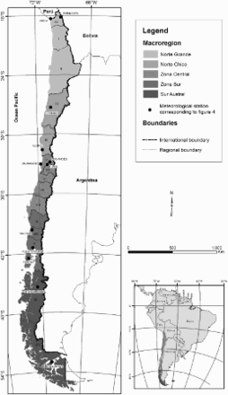
The study area is continental Chile which extends from ∼17°S to ∼56°S. Chile has 15 administrative regions (Figure 1), and 5 macroregions can be distinguished:

• Norte Grande Macroregion: comprising the administrative regions of Arica and Parinacota (XV), Tarapacá (I) and Antofagasta (II).

• Norte Chico Macroregion: comprising the administrative regions of Atacama (III) and Coquimbo (IV).

• Zona Central Macroregion: comprising the administrative regions of Valparaíso (V), Santiago (XIII), ÓHiggins (VI), Maule (VII) and Biobío (VIII).

• Zona Sur Macroregion: comprising the administrative regions of Araucanía (IX), Los Ríos (XIV) and Los Lagos (X).

• Sur Austral Macroregion: comprising the administrative regions of Aisén (XI) and Magallanes (XII).

Figure 1. Study area.

2.2. Climate surfaces for the Köppen–Geiger classification

The Köppen–Geiger climate classification for Chile was developed using the bioclimatic surfaces of Pliscoff, Luebert, Hilger, and Guisan (2014), refered to raster images with a resolution of 1 × 1 km for bioclimatic variables (Hutchinson, 1995) as well as for monthly precipitation and temperature during the period between 1950 and 2000. These climate surfaces were generated using the Anusplin software v.4.36 (Hutchinson, 2006; Xu & Hutchinson, 2013) which derives results from monthly precipitation and temperature variables as well as the 19 bioclimate surfaces described by Nix (1986). The climate surfaces were constructed in order to perform a bioclimatic analysis of ecological niches, by calculating the coefficient of variation, seasonality and temperature and annual range of precipitation. The climate surfaces were calculated for the period between 1950 and 2000 at the stations from the Global Historical Climate Network Dataset (GHCN), FAOClim 2.0 and those of other authors.

Five bioclimatic variables were used: BIO1 (mean annual temperature, MAT), BIO5 (mean temperature of the hottest month, Thot), BIO6 (mean temperature of the coldest month, Tcold), BIO7 (temperature annual range – BIO5–O6) and BIO12 (mean annual precipitation, MAP).

Both the summer (DJF) and winter (JJA) monthly data from Pliscoff et al. (2014) were used to establish the precipitation for the driest month of the year. The mean monthly temperature was used for the months for which the mean temperature is equal or greater than 10°C.

The specific criteria for determining each climate type to the third order are shown in the flow diagram in Figure 2.

Figure 2. Flow diagram. Köppen–Geiger climatic classification criteria. Source: Modified from Peel et al. (2007) and Rohli, Joyner, Reynolds, and Ballinger (2015). MAP,  mean annual precipitation; MAT, mean annual temperature; Thot, temperature of the hottest month; Tcold, temperature of the coldest month; Tmon₁₀= number of months where the temperature is above 10°C; Pdry, precipitation of the driest month; Psdry,  precipitation of the driest month in summer; Pwdry, precipitation of the driest month in winter; Pswet, precipitation of the wettest month in summer; Pwwet, precipitation of the wettest month in winter; Pthreshold, varies according to the following rules (if 70% the MAP occurs in winter then Pthreshold = 2 × MAT, if 70% the MAP occurs in summer then Pthreshold = 2 × MAT + 28, otherwise Pthreshold = 2 × MAT + 14). Summer or winter is defined as the warmer or cooler six-month period of October, November, December, January, February, March (ONDJFM) and April, May, June, July, August, September (AMJJAS), respectively.

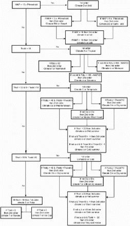
Because the climatic diversity of Chile cannot be differentiated in detail with only three orders, new criteria were applied to enable the identification of climatic subtleties:

• h (highland) climates: a discriminatory threshold elevation of 1000 m.a.s.l. was established for mediterranean climates; if we assume that temperature decreases with elevation at a gradient of 0.65°C/100 m, the thermal variation above 1000 m is considerable and, therefore, this elevation defines an appropriate limit for the classification of the Andes mountain range.

• ' (attenuated euoceanic) climates: only for semi-arid and temperate climates. This assumes the BIO7 climatic variable of Pliscoff et al. (2014) which enabled the definition of those climates whose temperature range does not exceed 16–17°C, in accordance with the Rivas-Martinez index (2004), and which implies a climate with a more pronounced oceanic influence (Amigo, Izco, de Compostela, & Rodriguez Guitián, 2007). This was created in order to highlight the cloudy coastal zone whose climate surface was not available for this study.

• w (dry winter) climates: used for the B, Cf and E climates. Enables the classification of all those climates having an Amazonian influence in the South American monsoon system.

• s (dry summer) climates: used for the B, Cf and E climates and enables the classification of all those climates with a dry summer.

The study of bioclimate surfaces was carried out using Esri ArcGIS 10.2 software.

2.3. Validation of the Köppen–Geiger classification

We performed a spatial comparison between the Köppen–Geiger classification applied to the surfaces and the classification obtained from the FAO Clim 2.0 (FAO, 2001) stations. The superposition enabled the detection of correspondences between the map and the locations of the stations.

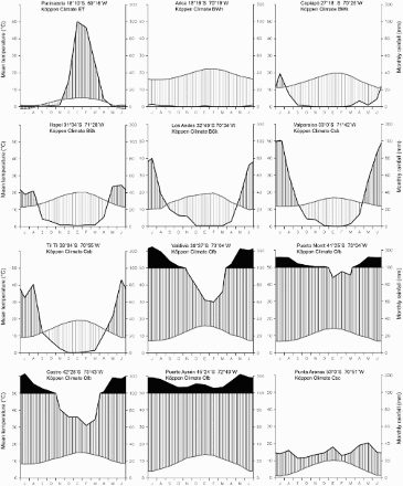
By way of illustration, Walter and Lieth diagrams were generated for 12 locations in Chile (see Figure 1), which are representative of its climatic diversity, in addition to the results of correspondences and lack of correspondence between the map and the points of the FAO – Clim stations.

3. Results

The principal product resulting from this study is the map showing the spatial distribution of Köppen–Geiger climate types with a resolution of 1 × 1 km, at a scale 1:2,000,000; this is presented as the Main Map in PDF format, and contains 25 Chilean climate types.

3.1. Synopsis of Köppen–Geiger classification map for continental Chile

Continental Chile has three first-order climates (B, C and E), which are distributed from north to south (arid, temperate and polar climates) and modulated by the elevation of the Andes (polar climates can be found in northern Chile). With regard to the first-order Köppen–Geiger classification, the prevailing climate, occurring in 41% of the region, is temperate (C), followed by the arid climate (B), which accounts for 31%, and finally, the remaining 28% has a polar climate (E).

The second-order Köppen–Geiger classification gives rise to six climates which, in order of importance, are: ET (27.9%), Cs (21.4%), Cf (19.7%), BW (18.2%), BS (12.7%) and EF (0.1%).

The nine third-order Köppen–Geiger classifications, in order of decreasing frequency, are: ET (27.9%), BWk (17%), Csb (16.3%), BSk (12.7%), Cfb (12.5%), Cfc (7.2%), Csc (5.2%), BWh (1.1%) and EF (0.1%).

When the climatic subtleties are taken into consideration, there are 25 climatic types occurring in continental Chile; these climates provide a better understanding of the origin of the air masses which affect their distribution, for example, with respect to elevation (h), isothermality (') or the dominance of westerly winds on concentrated winter rainfall (s) and easterly winds on concentrated summer rainfall (w). Climates with concentrated summer rainfall or with a dry winter season (w) are of interest, because they are specific to the Amazonian influence and affect the tundra, ice cap (glacial) and cold semi-arid climates, all of which occur on the northern Chilean plateau. The isothermal or attenuated euoceanic (') climates appear along the coast from Atacama (III Region), to Los Lagos (X Region), with an influence extending to between approximately 63 and 120 km inland.

3.2. First-order Köppen–Geiger classification by Macroregion

Norte Grande Macroregion: occurrence of B and E climates (arid and polar, the latter due to the elevation of the Andes which is over 3000 m above sea level) with no occurrence of the C (temperate) climates. The region is occupied by a higher proportion of arid or B climates (75%), specifically the desert climates (BW) typical of the Atacama Desert, which are the driest in the world (Robinson et al., 2015). In this area, the Amazonian influence occurs primarily at lower latitudes.

Norte Chico Macroregion: the predominance of arid or B (67%) and E or polar (29%) climates. The polar climates are located primarily at higher elevations in the Andes. The C climates, in turn, occupy the lowest percentage of the Norte Chico (4%). It should be noted that the Amazonian influence is still maintained in this macroregion.

Zona Central Macroregion: The most predominant climate is temperate (C) which occupies 91% of the entire macroregion. On the other hand, the regional occurrence of the E climates, which account for only a residual percentage (less than 6%), and are restricted to high mountain areas, decreases considerably. Arid climates occur in only 3% of the total area.

Zona Sur Macroregion: Temperate climates predominate at 97%, with tundra accounting for 2.5%. The Andes barely exceed 2000 m in elevation.

Sur Austral Macroregion: Polar (E) climates predominate with a 52% occurrence in the region. Due to leeward conditions and the elevation of the western islands, B climates occur at residual percentages of less than 5%. The C climates are distributed over approximately 44% of the region.

3.3. Geographic distribution of the Köppen–Geiger climate classifications

Desert climates predominate from ∼17°30'S to ∼28°15'S, with a wide variety of arid climates, specifically the BW climates from the coast to the Andes, and to a lesser extent, semi-arid climates. Variants of the high-elevation arid and tundra climates with an Amazonian influence (winter droughts, 4th order climates of type w) occur here. The types which are more affected by the continentality of Chile predominate due to the sparse vegetation and steep topography of the ‘Farellón Costero’ geomorphological unit. Of great interest is an understanding of how the warm desert climate (BWh) can be traced back to the coastal streams of Lluta, Azapa, Vitor, Camarones, Tana and Río Loa and extends to the Pampa del Tamarugal and Mejillones. Climates with an Amazonian influence (ET (w) and BSk (w)) extend from northern Chile to 27° 8'S, to the northeast of Ojos del Salado (6880 m), while the BWk (w) climates extend to 24° 21'S, widening from Calama to the Salar de Atacama.

Further south of 28°15'S and extending to 32°30'S, there is a predominance of semi-arid climates, specifically BSk, with its rainy winter (or summer drought, 4th order s climates) and summer rain (or winter drought, 4th order w climates) variants. In addition, the cold tundra climates are restricted to the considerably higher elevations of the Andes which, at these latitudes, sometimes exceed 6000 m.

The central region of the country, from 32°30'S to 39°32'S (Cerro Nilcahuin and Lake Calafquen) is dominated by temperate climates, specifically the mediterranean (Csb and Csc), with its isothermal (4th order Csb’ climates) and high-elevation (4th order Csb climates (h)) variants. An interesting aspect is that the north-western area (Batuco, Lampa) of the metropolitan region of Santiago, capital of Chile, and the foothills of the Andes, are classified as semi-arid.

Southern temperate climates (Cfb), classified as Marine West Coast, predominate from ∼39°32'S to approximately ∼43°S. In this area, the decreased elevation of the Andes, the influence of westerly winds, high rainfall and oceanic conditions determine the configuration of the Zona Sur macroregional climate. The Csb climates here exhibit a sub-mediterranean character (Rivas-Martínez, 2007).

The Zona Sur Austral exhibits a predominance of polar tundra climates and, to a lesser extent, those classified as EF. There is also an occurrence of Patagonian semi-arid climates (BSk) and sub-mediterranean climates (primarily Csc).

3.4. Results of the Köppen–Geiger classification applied to the weather stations

Of a total of 200 FAO Clim 2.0 weather stations for Chile, 194 were considered valid for analysis, as the rest of the stations occur outside of the South American landmass. These 194 stations were spatially coupled with the Köppen–Geiger climate classification map. The climatic classification method used is illustrated in Figure 2.

The coincidence of climatic classifications on the map with those of the stations is 80%. The results are presented in Figure 3 which illustrates the percentages of coincidence by region. Thirty-nine stations do not coincide with the climatic classification map, as according to a review of the FAO Clim 2.0 meta-data, they are not representative of the 1950–2000 period. Moreover, 20 of the 39 weather stations do not show any indication of the operational period of the climate station for the monthly temperature variable.

Figure 3. Correspondence of Köppen–Geiger climatic classification applied to data from weather stations with the macroregional level map.

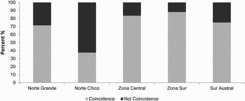
Figure 3 shows that, at the macroregional level, the South exhibits a higher degree of coincidence (88%) between the map and the weather stations. The macroregion exhibiting the least coincidence is the Norte Chico with only 37.5%, as the FAO Clim2.0 stations indicate BWk or desert climates, and the map indicates semi-arid climates (BSk).

Finally, Figure 4 shows the climatic variety of Chile, plotted in Walter and Lieth diagrams for 12 localities within the study area. Winter rainfall was observed to be the predominant precipitation pattern (except in the region of Parinacota, representative of the ET (w) climate), and the temperature decreases to the south while precipitation increases, except for Punta Arenas (due to its leeward situation).

Figure 4. Walter and Lieth diagrams for 12 Chilean localities.

4. Conclusions

Having an up-to-date climate map of Chile (1950–2000) with such a comprehensive classification system (despite its antiquity), such as that proposed by Köppen–Geiger, is of great geographic and climatic interest.

A novel conclusion is that the use of climate surfaces enables the generation of maps with discrete classifications and climatic indices which, when contrasted with data from weather stations, facilitates better approximations of the limits and of the spatial distribution of climates than in previous studies.

The singularities detected allow us to discern 25 types of climate for continental Chile based on the usual climatic and geographic criteria. Among these criteria are the concentration and origin of precipitation, the conditions of isothermality, the attenuated euoceanic behaviour of temperatures and the elevation of 1000 m above sea level.

Future studies are expected to add new information and improve the scale of the map. For example, one goal is to add cloud cover as an important climatic factor (particularly in the Norte Grande Macroregion), and to perform downscaling processes to 100 m by means of multiple regressions.

Software

The map was created using Esri ArcGIS 10.2 software on Pliscoff et al. (2014) climate surfaces, which were transformed by vector and exported to PDF.

Disclosure statement

No potential conflict of interest was reported by the authors.

ORCID

Pablo Sarricolea http://orcid.org/0000-0002-6679-2798

Óliver Meseguer-Ruiz http://orcid.org/0000-0002-2222-6137

Additional information

Funding

The authors gratefully acknowledge funding from Fondecyt Initiation [11130629], Fondecyt Regular [1150701 and 1151087], the Climatology Group at the University of Barcelona (Government of Catalonia) [2014SGR300], and Convenio de Desempeño UTA-MINEDUC.

References

- Alvares, C. A., Stape, J. L., Sentelhas, P. C., de Moraes, G., Leonardo, J., & Sparovek, G. (2013). Köppen’s climate classification map for Brazil. Meteorologische Zeitschrift, 22(6), 711–728. doi: 10.1127/0941-2948/2013/0507
- Amigo, J., Izco, J., de Compostela, S., & Rodriguez Guitián, M. A. (2007). Rasgos bioclimáticos del territorio templado de Chile. Phytocoenologia, 37(3–4), 739–751. doi: 10.1127/0340-269X/2007/0037-0739
- Beck, H. E., van Dijk, A. I., de Roo, A., Miralles, D. G., McVicar, T. R., Schellekens, J., & Bruijnzeel, L. A. (2016). Global-scale regionalization of hydrologic model parameters. Water Resources Research, 52(5), 3599–3622. doi: 10.1002/2015WR018247
- Belda, M., Holtanová, E., Halenka, T., & Kalvová, J. (2014). Climate classification revisited: From Köppen to Trewartha. Climate Research, 59(1), 1–13. doi: 10.3354/cr01204
- Chen, D., & Chen, H. W. (2013). Using the Köppen classification to quantify climate variation and change: An example for 1901–2010. Environmental Development, 6, 69–79. doi: 10.1016/j.envdev.2013.03.007
- FAO. (2001). FAOCLIM 2.0 a world-wide agroclimatic database. Rome: Food and Agriculture Organization of the United Nations.
- Fuenzalida-Ponce, H. (1971). Climatología de Chile, Departamento de Geofísica, Universidad de Chile 90 pp. Santiago, Chile
- Fuenzalida-Villegas, H. (1965). Clima. Geografía Económica de Chile, Corporación de Fomento de la Producción, Santiago, pp. 188–257.
- Hutchinson, M. F. (1995). Interpolating mean rainfall using thin plate smoothing splines. International Journal of Geographical Information Systems, 9(4), 385–403. doi: 10.1080/02693799508902045
- Hutchinson, M. F. (2006). ANUSPLIN version 4.36 user guide. Canberra: The Australian National University.
- Intergovernmental Panel on Climate Change (IPCC). (2013). Climate change 2013: The physical science basis. Contribution of working group I to the fifth assessment report of the intergovernmental panel on climate change. In T. F. Stocker, D. Qin, G.-K. Plattner, M. Tignor, S. K. Allen, J. Boschung, … P. M. Midgley (Eds.), (1535 pp.). Cambridge: Cambridge University Press.
- Kottek, M., Grieser, J., Beck, C., Rudolf, B., & Rubel, F. (2006). World map of the Köppen-Geiger climate classification updated. Meteorologische Zeitschrift, 15(3), 259–263. doi: 10.1127/0941-2948/2006/0130
- Nix, H. A. (1986). A biogeographic analysis of Australian elapid snakes. Atlas of Elapid Snakes of Australia, 7, 4–15.
- Peel, M. C., Finlayson, B. L., & McMahon, T. A. (2007). Updated world map of the Köppen-Geiger climate classification. Hydrology and Earth System Sciences Discussions, 4(2), 439–473. doi: 10.5194/hessd-4-439-2007
- Pliscoff, P., Luebert, F., Hilger, H. H., & Guisan, A. (2014). Effects of alternative sets of climatic predictors on species distribution models and associated estimates of extinction risk: A test with plants in an arid environment. Ecological Modelling, 288, 166–177. doi: 10.1016/j.ecolmodel.2014.06.003
- Rivas-Martínez, S. (2004). Global ioclimatics. Madrid: Phytosociological Research Center, Departamento di Biologia Vegetal II.
- Rivas-Martínez, S. (2007). Mapa de series, geoseries y geopermaseries de vegetación de España [Memoria del mapa de vegetación potencial de España]: Parte I [Salvador Rivas Martínez y colaboradores]. Itinera geobotanica, 17, 5–436.
- Robinson, C. K., Wierzchos, J., Black, C., Crits-Christoph, A., Ma, B., Ravel, J., … DiRuggiero, J. (2015). Microbial diversity and the presence of algae in halite endolithic communities are correlated to atmospheric moisture in the hyper-arid zone of the Atacama Desert. Environmental Microbiology, 17(2), 299–315. doi: 10.1111/1462-2920.12364
- Rohli, R. V., Joyner, T. A., Reynolds, S. J., & Ballinger, T. J. (2015). Overlap of global Köppen-Geiger climates, biomes, and soil orders. Physical Geography, 36(2), 158–175. doi: 10.1080/02723646.2015.1016384
- Rubel, F., & Kottek, M. (2010). Observed and projected climate shifts 1901–2100 depicted by world maps of the Köppen-Geiger climate classification. Meteorologische Zeitschrift, 19(2), 135–141. doi: 10.1127/0941-2948/2010/0430
- Sparovek, G., De Jong Van Lier, Q., & Dourado Neto, D. (2007). Computer assisted Koeppen climate classification: A case study for Brazil. International Journal of Climatology, 27(2), 257–266. doi: 10.1002/joc.1384
- Xu, T., & Hutchinson, M. F. (2013). New developments and applications in the ANUCLIM spatial climatic and bioclimatic modelling package. Environmental Modelling & Software, 40, 267–279. doi: 10.1016/j.envsoft.2012.10.003
- Zhang, L., Wang, C., Li, X., Cao, K., Song, Y., Hu, B., … Cao, S. (2016). A new paleoclimate classification for deep time. Palaeogeography, Palaeoclimatology, Palaeoecology, 443, 98–106. doi: 10.1016/j.palaeo.2015.11.041