Organic carbon and total nitrogen topsoil stocks, biogenetic natural reserve ‘Marchesale’ (Calabria region, southern Italy)

ABSTRACT

It is essential estimating the spatial distribution of soil organic carbon (SOC) and soil total nitrogen (STN) stocks and their spatial-temporal variations to understand the role of soil in ecosystem services and in the global cycles of carbon and nitrogen. This work was aimed to quantify and map the stocks of SOC and STN in topsoils in an area of the Biogenetic Natural Reserve ‘Marchesale’ (Calabria region, southern Italy). Forest soil samples (0–20 cm depth) were collected at 231 locations and analysed in laboratory for SOC and STN. Moreover, in all samples, bulk density (BD) and soil coarse fragments (SCFs) were determined. Geostatistics was used to map all soil properties (SOC, STN, BD and SCFs) and the stocks of SOC and STN. The mean stock values were 86.3 Mg ha⁻¹ for SOC and 5.1 Mg ha⁻¹ for STN. The total amounts stored in the study area (33.2 ha) were 2865.2 Mg for SOC and 170.1 Mg for STN. Although only the topsoil was considered, the accompanying maps (1:4000 scale) will be useful for the sustainable management of the Biogenetic Natural Reserve ‘Marchesale’ and for undertaking appropriate conservation plans to mitigate the emissions of greenhouse gases.

KEYWORDS:

• Forest soils
• organic carbon stock
• total nitrogen stock
• geostatistics
• GIS
• southern Italy

1. Introduction

Soil is a key component of terrestrial ecosystems generating a multitude of functions that support the delivery of ecosystems functions (Blum, 2005; CEC, 2006; Hannam & Boer, 2004; Palm, Sanchez, Ahamed, & Awiti, 2007).

In spite of the importance of soil, ecosystem services have been described with little emphasis on soil (Costanza et al., 1997; De Groot, Wilson, & Boumans, 2002; MEA, 2005). It is very important to link both soil properties (i.e. carbon, biota, nutrient cycling and moisture retention) and soil distribution for ecosystem services (Barrios, 2007; Ghaley, Porter, & Sandhu, 2014; Khanna, Oenal, Dhungana, & Wander, 2010; Krishnaswamy et al., 2013; Marks et al., 2009; Van Eekeren et al., 2010; Williams & Hedlund, 2013).

Maps of soil properties and processes at suitable resolutions are essential for modelling ecosystem services at different scales (Palm et al., 2007). In addition, information on chemical and physical soil properties and their spatial distribution is useful to characterize development and/or degradation conditions of soils (Conforti et al., 2013; Lal, 2004). In particular, soil organic carbon (SOC) and soil total nitrogen (STN) are important properties both for assessing pedogenetic processes and soil quality (Pan, Birdsey, Hom, & McCullough, 2009), and defining soil functions which determine the delivery of ecosystem services (Ghaley et al., 2014; Khanna et al., 2010). SOC and STN also play a key role as sources and sinks in global carbon and nitrogen cycles (Lal, 2004). The biogeochemical cycles of carbon and nitrogen in terrestrial ecosystems have received increasing attention worldwide over the last two decades because their emission into the atmosphere contributes greatly to global warming (Fu, Shao, Wei, & Robertm, 2010). Soils are the major terrestrial sink of organic carbon and about 1500 PgC are stored in the first metre of the soil (Batjes, 1996). Approximately 66% of the estimated global organic carbon is stored in forest soils (Dixon et al., 1994; Jobbagy & Jackson, 2000). The spatial variation of SOC stocks in different forest ecosystems (e.g. boreal, temperate and tropical) is controlled by several environmental factors such as latitude, air temperature, precipitation regime, topographic relief, vegetation species, primary productivity, quantity and quality of litter, soil types, soil moisture regime and soil microbial activity (Batjes, 1996; Cambule, Rossiter, Stoorvogel, & Smaling, 2014; Conforti, Lucà, Scarciglia, Matteucci, & Buttafuoco, 2016; Fantappiè, L'Abate, & Costantini, 2011; Fu et al., 2010; Ganuza & Almendros, 2003; Jobbagy & Jackson, 2000; Kunkel, Flores, Smith, McNamara, & Benner, 2011; Lal, 2005; Liu et al., 2006; Marty, Houle, & Gagnon, 2015; Stevenson, 1999; Takata, Funakawa, Akshalov, Ishida, & Kosaki, 2007; Telles et al., 2003; Thompson & Kolka, 2005; Wang, Zhang, Zhang, & Li, 2009; Yimer, Ledin, & Abdelkadir, 2006). Changes in land use and forest management practices can also have significant effects on SOC pools (Fu et al., 2010; Jobbagy & Jackson, 2000; Lal, 2005). It has been recognized that small fluctuations of the SOC pool could have large impacts on the atmospheric CO₂ concentration (Lal, 2004; Powlson, Whitmore, & Goulding, 2011). Therefore, mapping stocks of SOC and STN, and identifying the environmental factors controlling their spatial variability is important for identifying, quantifying and understanding natural carbon and nitrogen sinks to mitigate the effects of climate change (Jobbagy & Jackson, 2000; Lal, 2005; Yang, Luo, & Finzi, 2011; Yimer et al., 2006). Many studies have also analysed the spatial variability of SOC and STN distribution and stocks at different spatial scales (e.g. Grimm, Behrens, Märker, & Elsenbeer, 2008; Kumar, Lal, & Liu, 2012; Liu et al., 2006; Rodríguez Martín et al., 2016; Thompson & Kolka, 2005; Wang, Fu, Lu, Song, & Luan, 2010; Wiesmeier et al., 2014).

The objective of this study is to quantify and map the stocks of organic carbon and total nitrogen in forest topsoils in an area of the Biogenetic Natural Reserve ‘Marchesale’ (Calabria region, southern Italy).

2. Material and methods

2.1. Study area

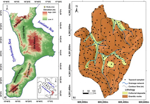
The study area is a Natura 2000 site in the Biogenetic Nature Reserve ‘Marchesale’, in the Calabria region (southern Italy), between 38° 30′ 7″ N and 38° 29′ 31″ N and 16° 14′ 10″ E to 16° 14′ 42″ E (Figure 1(a)). The study area is about 33.2 ha in area and is covered by a high forest of beech (Fagus sylvatica L.), sometimes mixed with silver fir (Abies alba Mill.) trees (Conforti et al., 2016). Elevation ranges from 1137 to 1212 m above sea level and slopes vary from 0° to about 45° (mean 10°) and the predominant slope aspects are north and west.

Figure 1. (a) Location of study area and (b) lithologic map and topsoil sampling locations.

Climate is Mediterranean upland (Csb-type, sensu Köppen, 1936) with a mean annual precipitation of about 1800 mm, concentrated mainly from November to February. The annual mean temperature is 11.3°C with a mean maximum value of 28.3°C in summer and a mean minimum value of −3.7°C in winter (Conforti et al., 2016).

Geologically the study area lies in the Serre Massif, where Palaeozoic granitoid rocks outcrop. These rocks are strongly jointed, weathered and frequently covered by thick regolith some of which are colluvial deposits (Calcaterra, Parise, & Dattola, 1996; Conforti, Froio, Matteucci, & Buttafuoco, 2015).

The landscapes of the study area are characterized by summit paleosurfaces, which represent the residual flat or gently sloping highlands, often separated by steep slopes with deep V-shaped valleys (Calcaterra & Parise, 2010; Conforti et al., 2016; Lucà, Robustelli, Conforti, & Fabbricatore, 2011).

The soils developed over this area were classified according to the USDA (2014) as Inceptosols (Humic Dystrudept) and Entisols (Lithic Udipsamments) and are heavily dependent on the nature of the parent rock and topographic features (Conforti et al., 2016). Soil depth ranges from shallow to moderately deep (0.2–1 m) with profiles characterized by A-Bw-Cr horizons and/or A-Cr horizons (ARSSA, 2003). The A horizon shows a very dark brown colour due to the high accumulation of organic matter (Umbric epipedon, USDA, 2014); moreover, these soils have acidic pH varying between 4.0 and 5.3 (Conforti et al., 2016).

2.2. Data collection and analysis

Topsoil (0–20 cm depth) samples were collected at 231 locations, between September and October 2012 (Figure 1(b)); at the same time, undisturbed soil samples to measure bulk density (BD) were collected using a metallic core cylinder with a diameter of 7.5 cm and a length of 20 cm (883.13 cm³). The limit of the top 20 cm of the soil was chosen because it often represents the limit of the A horizons measured from the base of the organic horizons (Conforti et al., 2016), which were removed. All the coordinates of the sampling locations were determined using a global positioning system receiver with a precision of about 1 m. The sampling strategy was to collect representative data of the various landforms of the study area.

Each soil core was oven dried at 105°C until constant weight. Soil BD was calculated as the ratio of the dry weight and the metallic core volume.

The disturbed soil samples were air-dried, gently crushed and passed through a 2-mm mesh sieve to collect the fine earth fraction; gravels (diameter >2 mm) were weighed to obtain the volumetric percentage of soil coarse fragments (SCFs).

The fine earth, after a pre-treatment with sodium hexametaphosphate as a dispersant, was analysed for particle size distribution (sand, silt and clay fractions) using the hydrometer method (Patruno, Cavazza, & Castrignanò, 1997). The particle size distribution was then classified in accordance with the soil texture triangle of the United States Department of Agriculture (USDA). SOC and STN concentrations were determined by dry combustion at 900° of subsamples of soil (5 mg), previously sieved at 0.25 mm, using the Elemental Analyzer NA 1500 (Carlo Erba Instruments, Milan, Italy).

Stocks of SOC and STN were determined using the following equations:(1) $\text{SOC stock}=\frac{\text{SOC}\times D\times BD\times (1-\text{SCFs}/100)}{10},$(1) (2) $\text{STN stock}=\frac{\text{STN}\times D\times BD\times (1-\text{SCFs}/100)}{10},$(2) where SOC (g kg⁻¹) is soil organic carbon and STN is soil total nitrogen concentration (g kg⁻¹); D is layer thickness (20 cm) of the topsoil, BD (g cm⁻³) is soil bulk density and SCFs is soil coarse fragments content (% of volume) using an average rock density of 2.65 g cm⁻³ (USDA, 2014).

All input variables (SOC, STN, BD and SCFs) were spatially predicted using a geostatistical approach before the determination of both stocks to reduce the propagation of errors in input data through Equations (1) and (2). Successively, the Equations (1) and (2) were implemented in a geographic information system (GIS) to calculate SOC and STN stocks.

2.3. Geostatistical approach

Every input variable (SOC, STN, BD and SCFs) was modelled as an intrinsic stationary process. For every soil property, each datum z(x_α) at different location x_α (x is the location coordinates vector and α the sampling points = 1, … , N) was interpreted as a particular realization of a random variable Z(x_α).

The quantitative measure of spatial correlation of the regionalized variable z(x_α) is the experimental variogram γ(h) which is a function of the distance vector (h) of data pair values [z(x _α), z(x_α+ h)]. A theoretical function, called the variogram model, is fitted to the experimental variogram to allow estimation of the variogram analytically for any distance h. Experimental variograms can be modelled using only functions that are conditionally negatively defined, in order to ensure the non-negativity of the variance of the prediction error. The objective is to build a permissible model that captures the main spatial features of the attribute under study. The variogram model generally requires two parameters: range and sill. The range is the distance over which pairs of the analysed soil property values are spatially correlated, while the sill is the variogram value corresponding to the range. The optimal fitting is chosen on the basis of cross-validation, which checks the compatibility between the data and the structural model considering each data point in turn, removing it temporarily from the data set and using its neighbouring information to predict the value of the variable at its location. The estimate is compared with the measured value by calculating the experimental error, that is, the difference between estimate and measurement, which can also be standardized by estimating the standard deviation. The goodness of fit was evaluated by the mean error (ME) and the mean squared deviation ratio (MSDR). The ME proves the unbiasedness of the estimate if its value is close to 0, while the MSDR is the ratio between the squared errors and the kriging variance (Webster & Oliver, 2007). If the model for the variogram is accurate, the mean squared error should equal the kriging variance and the MSDR value should be 1.

The fitted variograms were used to estimate each soil property values at unsampled locations using ordinary kriging (Webster & Oliver, 2007) at the nodes of a 1 m × 1 m interpolation grid.

In the geostatistical approach, even though the data are not required to follow a normal distribution, variogram modelling is sensitive to strong departures from normality, because a few exceptionally large values may contribute to many very large squared differences. In this case, the multi-Gaussian approach allows prediction at unsampled locations regardless of the shape of the sample histogram (Verly, 1983). It is based on a multi-Gaussian model and requires a prior Gaussian transformation of the initial soil property values into a Gaussian-shaped variable with zero mean and unit variance. Such a procedure, which is known as Gaussian anamorphosis (Chilès & Delfiner, 2012; Wackernagel, 2003), is a mathematical function that transforms a variable with a Gaussian distribution into a new variable with any distribution. The Gaussian anamorphosis can be achieved using an expansion into Hermite polynomials (Wackernagel, 2003) restricted to a finite number of terms. The kriging results must be back-transformed to the raw distribution afterwards. All statistical and geostatistical analyses were performed using ISATIS^® 2016.1 (www.geovariances.com).

The input variables (SOC, STN, BD and SCFs) were used to compute (Equations (1) and (2)) and map the spatial distribution of SOC and STN stocks. The two maps were compiled at 1:4000 scale (Main Map) using GIS software. The simplified topographic map with a 5 m contour interval, derived from a digital elevation model (DEM), was used. The values of SOC and STN stocks were reclassified into five classes by means of the natural-breaks method (Jenks, 1989). This technique identifies break points by picking the class that breaks the best group in similar values, maximizing the differences between classes.

3. Results and discussion

Descriptive statistics for the physico-chemical soil properties of the 231 topsoils sampled in the study area are showed in Table 1. Only SCFs depart from normality (a positive skewness of 1.23; Table 1) and has been transformed using the Gaussian anamorphosis. The percentage of SCFs ranged from 1.5% to 53.5%, with a mean value of 16.2% (Table 1). The soil texture was dominated by sand and silt, on average more than 85%, while the clay content was very low, with a mean value of 11.8%. From the USDA soil texture triangle (Figure 2), the following four soil texture classes were observed in the study area: silt loam, loam, sand loamy and loamy sand, indicating a presence of coarse and medium-textured soils in the study area. The mean BD value was 0.9 g cm⁻³, with values ranging from 0.5 to and 1.4 g cm⁻³ (Table 1).

Figure 2. Distribution of sand, silt and clay of the topsoil samples in the USDA textural triangle.

Table 1. Summary statistics of the soil properties.

Soil properties	Min	Max	Mean	Median	Lower quartile	Upper quartile	Std. dev.	Skewness (–)	Kurtosis (–)
SCFs (%)	1.5	53.5	16.2	14.2	9.7	20	9.5	1.23	1.90
Sand (%)	17.2	81.1	43.9	43.3	35.1	52.1	11.5	0.43	0.06
Silt (%)	15.9	69.8	44.3	44.7	37.2	52.2	10.6	−0.37	−0.25
Clay (%)	2.8	24.9	11.8	11.6	9.0	14.0	3.9	0.37	0.32
BD (g cm^−3)	0.5	1.4	0.9	0.9	0.7	1	0.2	0.20	0.61
SOC (g kg^−1)	14.5	141.0	62.2	62.9	50.8	73.8	18.6	0.28	1.38
STN (g kg^−1)	0.8	7.7	3.7	3.6	2.9	4.5	1.2	0.35	0.15

Note: Std. dev: standard deviation.

SOC concentration showed considerable variation with a range of 126.5 g kg⁻¹ and a mean of 62.2 g kg⁻¹, indicating that most topsoil samples have a high SOC concentration, related to the continuous supply of carbon provided by the decomposition of litter (Conforti et al., 2016). The STN concentration covered a range from 0.8 to 7.7 g kg⁻¹ with mean and median values of 3.7 and 3.6 g kg⁻¹, respectively (Table 1).

The results of the Pearson’s correlation analyses of the seven soil properties analysed are given in Table 2. As expected, significant positive correlation was found between STN and SOC (r = 0.87, p < .01). Also, SOC and STN were significantly correlated with particle size distribution (sand, silt and clay content) and BD (Table 2). In agreement with many studies (e.g. Konen, Burras, & Sandor, 2003; Lopes et al., 2015; Telles et al., 2003), the negative correlation between SOC, STN and sand content was expected, because, generally, soils with a high content of sand are well aerated and tend to have low soil moisture content, which is due to a rapid decomposition and a low stabilization of the organic carbon (Baritz, Seufert, Montanarella, & Van Ranst, 2010; Telles et al., 2003). The significant and negative correlation between SOC and BD confirmed by many studies (e.g. Conforti et al., 2016; Evrendilek, Celik, & Kilic, 2004; Hati, Swarup, Dwivedi, & Bandyopadhyay, 2007; Wang et al., 2011), indicates that SOC concentrations increased with decreasing BD; therefore, the cause of lower BD when soils are very rich in organic carbon can be related to their low specific density (Ma, Zhang, Tang, & Liu, 2016).

Table 2. Pearson’s correlation among soil properties analysed in the study area.

Variable	SCFs	Sand	Silt	Clay	BD	SOC	STN
SCFs	1.00	–	–	–	–	–	–
Sand	0.44**	1.00	–	–	–	–	–
Silt	−0.37**	−0.94**	1.00	–	–	–	–
Clay	−0.29**	−0.38**	0.08	1.00	–	–	–
BD	0.33**	0.43**	−0.29**	−0.56**	1.00		–
SOC	0.02	−0.41**	0.38**	0.19*	−0.54**	1.00	–
STN	−0.02	−0.38**	0.34**	0.21*	−0.55**	0.87**	1.00

*Significant at p < .05.

**Significant at p < .01.

To analyse the spatial continuity of the soil properties in all the directions of the space and especially to identify the possible anisotropies, for each property a map of the 2D variograms (not shown) was computed. No relevant difference as a function of direction (anisotropy) was showed and the experimental variograms looked upper bounded. Then, bounded isotropic nested variogram models were fitted for each input soil property (Table 3, Figure 3).

Figure 3. Experimental variograms (filled circle) and fitted models (solid line) for SOC, nitrogen, BD and coarse fragments. Experimental variance (horizontal dashed line) is also reported.

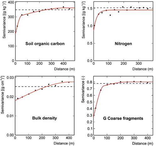
Table 3. Parameters of variogram models for the input variables, and results of cross-validation.

Variable	Model	Sill	Range (m)	ME	MSDR
SOC (g kg^−1)	Nugget	182.38	–	0.2771	1.05
	Spherical	116.01	52.04
	Spherical	63.42	418.18
STN (g kg^−1)	Nugget	0.8681	–	0.0358	1.02
	Exponential	0.5912	186.72^a
BD (g cm^−3)	Nugget	0.0180	–	−0.0008	1.03
	Spherical	0.0097	418.86
G SCFs (–)	Nugget	0.2692	–	−0.0047	1.05
	Spherical	0.4288	76.79
	Spherical	0.1033	257.24

Note: ME = mean estimate error and MSDR = mean squared deviation ratio.

^aEffective range.

For SOC and G SCFs, the fitted models included a nugget effect and two spherical models (Webster & Oliver, 2007): one at short range and the other at long range (Table 3). This means that a spatial dependence of SOC and G SCFs data occurred at two distinct spatial scales. The nugget effect (Webster & Oliver, 2007) implies a positive intercept of the variogram. It arises from errors of measurement and spatial variation within the shortest sampling interval (Webster & Oliver, 2007).

The fitted model for STN data also included a nugget effect and an exponential model (Webster & Oliver, 2007), while the fitted model for BD included a nugget effect and a spherical model. The exponential model approaches its sill asymptotically and then it does not have a finite range. Generally, for practical purposes it is convenient to assign it an effective range and this is usually taken as the distance at which the variogram equals 95% of the sill variance.

The goodness of fit for the variogram models was verified by cross-validation and the statistics used, that is, the mean of the estimation error and variance of the mean squared deviation ratio, showed satisfactory results (quite close to 0 and 1, respectively) (Table 3). The above variogram models were used with ordinary kriging and ordinary multi-Gaussian kriging to produce the maps of the four variables input (Main Map).

3.1. Spatial distribution of SOC and STN stocks

The Main Map shows the spatial patterns of SOC and STN stocks. The map of SOC stock displayed high spatial variability ranging from 33 to 132 Mg ha⁻¹, with a mean of 86.3 Mg ha⁻¹ and a standard deviation of 9.7 Mg ha⁻¹. The mean SOC stock is consistent with the values obtained for forest soils in other studies carried out both in Italy (Faggian, Bini, & Zilioli, 2012; Garlato et al., 2009; Solaro & Brenna, 2005) and in others European countries (e.g. Baritz et al., 2010; Rodríguez Martín et al., 2016; Sariyildiz, Savaci, & Kravkaz, 2016; Wiesmeier et al., 2014).

About 63% of the study area was estimated to have an SOC stock of between 82 and 98 Mg ha⁻¹, about 10% was higher than 98 Mg ha⁻¹, and the remaining 27% was lower than 82 Mg ha⁻¹. The amount of SOC storage estimated within the whole study area was 2865.2 Mg to a depth of 20 cm.

With regard to the spatial distribution of STN stock, the mean was 5.1 Mg ha⁻¹ and standard deviation of 0.5 Mg ha⁻¹, with STN stock values ranging from 3.9 to 7.9 Mg ha⁻¹. In more than 76% of the study area the STN stored in the topsoil has a value between 4.6 and 5.8 Mg ha⁻¹. The map shows that the zones with lowest STN stocks (ranging between 3.9 and 4.6 Mg ha⁻¹) accounted for about 15% of the study area, whereas the highest values (ranging from 5.6 to 7.9 Mg ha⁻¹) constituted 9% of the study area. For the whole study area, the value of the total STN stored in the upper 20 cm was 170.1 Mg.

The values of STN stock in the study area are comparable with those reported by Sariyildiz et al. (2016) for forest topsoils of north-western Turkey (5.93 Mg ha⁻¹) and by Vesterdal, Schmidt, Callesen, Nilsson, and Gundersen (2008) for surface soils in a beech forest of Denmark (4.50 Mg ha⁻¹).

The maps showed that the spatial distribution patterns of both SOC and STN stocks were comparable. Moreover, the two maps showed that the spatial pattern of SOC stock was significantly correlated (r = 0.70, p < .001) with STN stock map, thus suggesting that the latter generally had the same behaviour as SOC storage, due to the fact that most nitrogen forms are part of the soil organic matter, which is the primary sink of STN (Ganuza & Almendros, 2003).

Since a forest is a dynamic system continuously changing, the results of this study can support foresters to make decisions about forest management plans. In fact, information and maps of soil properties for forest lands are required in order to make good management decisions to promote carbon sequestration and conservation of biodiversity in forest soils.

4. Conclusions

In this study, a geostatistical approach and GIS analysis allowed mapping of the spatial variability of SOC and STN stocks in a representative site within the Biogenetic Natural Reserve ‘Marchesale’, located in Calabria region (southern Italy) (Main Map).

The input variables used to compute the stocks of SOC and STN (SOC, STN, BD and SCFs) were first interpolated using a geostatistical approach and then used to produce the maps of stocks of SOC and STN (Main Map).

The maps showed that within the top 20 cm of soil, SOC and STN stocks have a high spatial variability (Main Map). The results indicated that mean values of SOC and STN stocks estimated were 86.3 and 5.1 Mg ha⁻¹, respectively. The total amount of SOC stored was 2865.2 Mg whereas the total STN stock was 170.1 Mg.

This study has provided the first detailed knowledge about the spatial pattern of SOC and STN stored, at local scale, in the forest topsoils of the Calabria region. Moreover, SOC and STN storage are important not only because of their role in the global carbon and nitrogen cycles, but also because they affect forest productivity and ecological functioning. Finally, the maps can also be used as support to develop sustainable management strategies in forest ecosystems, which in Calabria cover about 40% of the territory.

Software

Statistical and geostatistical analysis were carried out using Isatis^® 2016.1. ESRI ArcGIS 9.3 software was used for management the data, for the production of soil properties maps, and to assemble the layout of Main Map.

Map design

We present a maps of SOC and total nitrogen stocks for an area of the Biogenetic Natural Reserve ‘Marchesale’ (Calabria region, south Italy). The spatial pattern of organic carbon and total nitrogen stocks (Mg ha⁻¹) was calculated as the product of the following soil properties: SOC and STN concentration, BD and soil course fragments, which were interpolated by means geostatistical approach; in particular, ordinary kriging method was used. All geostatistical analyses were performed with the software Isatis^®, release 2016.1 (http://www.geovariances.com). Each map of the soil properties were compiled at 1:8000 scale, using a GIS software. Successively, the following equations were implemented in a GIS for calculate SOC and STN stocks:(1) $\text{SOC stock = }\frac{\text{SOC}\times D\times BD\times (1-\text{SCFs}/100)}{10},$(1) (2) $\text{STN stock}=\frac{\text{STN}\times D\times BD\times (1-\text{SCFs}/100)}{10},$(2) where SOC and STN are the soil organic carbon and total nitrogen concentration (g kg⁻¹), respectively, D is layer thickness (20 cm) of the topsoil, BD is the soil bulk density (g cm⁻³) and SCFs is the coarse fragments content expressed as percentage in volume.

The spatial distribution of SOC and STN stocks was calculated applying the Equations (1) and (2), respectively, and the cartographic representation of the two maps was performed on a scale 1:4000, using a GIS software. The simplified topographic map with a 5-m contour interval, derived from DEM, was used. The values of SOC and STN stocks were reclassified into five classes by means of the natural-breaks method.

The topographic base, with a 5-m contour interval, results from a DEM obtained by digitization of contour lines and points of the 1:5000 scale topographic maps.

All the maps, displayed in the Main Map, were transformed in vector format.

The topographic base, soil properties maps, SOC stock map, STN stock map and related layout were drafted using the ESRI ArcGIS 9.3.

Acknowledgements

The authors thank the three reviewers (Dr Makram Murad-al-shaikh, Dr Claudia Scopesi and Dr Vanessa Wong) and Associate Editor Dr Colin Pain for their critical comments and suggestions, which greatly improved the quality of our manuscript and map.

Disclosure statement

No potential conflict of interest was reported by the authors.

Additional information

Funding

The research was supported by the LIFE09 ENV/IT/000078 ManFor C.BD. ‘Managing forests for multiple purposes: carbon, biodiversity and socio-economic wellbeing’.

References

- ARSSA. (2003). Carta dei suoli della regione Calabria – scala 1:250000. Monografia divulgativa. ARSSA – Agenzia Regionale per lo Sviluppo e per i Servizi in Agricoltura, Servizio Agropedologia. Rubbettino, 387 pp.
- Baritz, R., Seufert, G., Montanarella, L., & Van Ranst, E. (2010). Carbon concentrations and stocks in forest soils of Europe. Forest Ecology and Management, 260, 262–277. doi: 10.1016/j.foreco.2010.03.025
- Barrios, E. (2007). Soil biota, ecosystem services and land productivity. Ecological Economic, 64, 269–285. doi: 10.1016/j.ecolecon.2007.03.004
- Batjes, N. H. (1996). Total carbon and nitrogen in the soils of the world. European Journal of Soil Science, 47, 151–163. doi: 10.1111/j.1365-2389.1996.tb01386.x
- Blum, W. E. H. (2005). Functions of soil for society and the environment. Reviews in Environmental Science and Biotechnology, 4, 75–79. doi: 10.1007/s11157-005-2236-x
- Calcaterra, D., & Parise, M. (2010). Weathering in the crystalline rocks of Calabria, Italy, and relationships to landslides. In D. Calcaterra & M. Parise (Eds.), Weathering as predisposing factor to slope movements (pp. 105–130). London: Geological Society of London, Engineering Geology Series, Special Publication, 23.
- Calcaterra, D., Parise, M., & Dattola, L. (1996). Caratteristiche dell’alterazione e franosità di rocce granitoidi nel bacino del torrente Alaco (Massiccio della Serre, Calabria). Bollettino della Società Geologica Italiana, 115, 3–28.
- Cambule, A. H., Rossiter, D. G., Stoorvogel, J. J., & Smaling, E. M. A. (2014). Soil organic carbon stocks in the Limpopo National Park, Mozambique: Amount, spatial distribution and uncertainty. Geoderma, 213, 46–56. doi: 10.1016/j.geoderma.2013.07.015
- CEC. (2006). Communication from the Commission to the Council (CEC), the European Parliament, the European Economic and Social Committee and the Committee of the Regions: Thematic Strategy for Soil Protection. Commission of the European Communities, COM, Brussels, p. 231.
- Chilès, J. P., & Delfiner, P. (2012). Geostatistics: Modelling spatial uncertainty. New York, NY: Wiley.
- Conforti, M., Buttafuoco, G., Leone, A. P., Aucelli, P. P. C., Robustelli, G., & Scarciglia, F. (2013). Studying the relationship between water-induced soil erosion and soil organic matter using Vis–NIR spectroscopy and geomorphological analysis: A case study in a Southern Italy area. Catena, 110, 44–58. doi: 10.1016/j.catena.2013.06.013
- Conforti, M., Froio, R., Matteucci, G., & Buttafuoco, G. (2015). Visible and near infrared spectroscopy for predicting texture in forest soil: An application in Southern Italy. iForest, 8, 339–347. doi: 10.3832/ifor1221-007
- Conforti, M., Lucà, F., Scarciglia, F., Matteucci, G., & Buttafuoco, G. (2016). Soil carbon stock in relation to soil properties and landscape position in a forest ecosystem of Southern Italy (Calabria region). Catena, 144, 23–33. doi: 10.1016/j.catena.2016.04.023
- Costanza, R., d’Arge, R., de Groot, R., Farber, S., Grasson, M., Hannon, B., … Van Den Belt, M. (1997). The value of the world's ecosystem services and natural capital. Nature, 387, 253–260. doi: 10.1038/387253a0
- De Groot, R., Wilson, M. A., & Boumans, R. M. J. (2002). A typology for the classification, description and valuation of ecosystem functions, goods and services. Ecological Economic, 41, 393–408. doi: 10.1016/S0921-8009(02)00089-7
- Dixon, R. K., Brown, S., Houghton, R. A., Solomon, A. M., Trexler, M. C., & Wisniewski, J. (1994). Carbon pools and flux of global forest ecosystems. Science, 263, 185–190. doi: 10.1126/science.263.5144.185
- Evrendilek, F., Celik, I., & Kilic, S. (2004). Changes in soil organic carbon and other physical soil properties along adjacent Mediterranean forest, grassland, and cropland ecosystems in Turkey. Journal of Arid Environment, 59, 743–752. doi: 10.1016/j.jaridenv.2004.03.002
- Faggian, V., Bini, C., & Zilioli, D. (2012). Carbon stock evaluation from topsoil of forest stands in NE Italy. International Journal of Phytoremediation, 14, 415–428. doi: 10.1080/15226514.2011.620656
- Fantappiè, M., L'Abate, G., & Costantini, E. A. C. (2011). The influence of climate change on the soil organic carbon content in Italy from 1961 to 2008. Geomorphology, 135, 343–352. doi: 10.1016/j.geomorph.2011.02.006
- Fu, X. L., Shao, M. A., Wei, X. R., & Robertm, H. (2010). Soil organic carbon and total nitrogen as affected by vegetation types in Northern Loess Plateau of China. Geoderma, 155, 31–35. doi: 10.1016/j.geoderma.2009.11.020
- Ganuza, A., & Almendros, G. (2003). Organic carbon storage in soils of the Basque Country (Spain): The effect of climate, vegetation type and edaphic variables. Biology and Fertility of Soils, 37, 154–162.
- Garlato, A., Obber, S., Vinci, I., Mancabelli, A., Parisi, A., & Sartori, G. (2009). La determinazione dello stock di carbonio nei suoli del Trentino a partire dalla banca dati della carta dei suoli alla scala 1:250.000. Studi Trentini di Scienze Naturali, 85, 157–160. (in Italian.)
- Ghaley, B. B., Porter, J. R., & Sandhu, H. S. (2014). Soil-based ecosystem services: A synthesis of nutrient cycling and carbon sequestration assessment methods. International Journal of Biodiversity Science, Ecosystem Services & Management, 10, 177–186. doi: 10.1080/21513732.2014.926990
- Grimm, R., Behrens, T., Märker, M., & Elsenbeer, H. (2008). Soil organic carbon concentrations and stocks on Barro Colorado Island – digital soil mapping using random forests analysis. Geoderma, 146, 102–113. doi: 10.1016/j.geoderma.2008.05.008
- Hannam, I., & Boer, B. (2004). Drafting legislation for sustainable soils: A guide. Gland: IUCN.
- Hati, K. M., Swarup, A., Dwivedi, A. K., & Bandyopadhyay, K. K. (2007). Changes in soil physical properties and organic carbon status at the topsoil horizon of a vertisol of central India after 28 years of continuous cropping, fertilization and manuring. Agriculture Ecosystems and Environment, 119, 127–134. doi: 10.1016/j.agee.2006.06.017
- Jenks, G. F. (1989). Geographic logic in line generalization. Cartographica, 26, 27–42. doi: 10.3138/L426-1756-7052-536K
- Jobbagy, E. G., & Jackson, R. B. (2000). The vertical distribution of organic carbon and its relation to climate and vegetation. Ecological Applications, 10, 423–436. doi: 10.1890/1051-0761(2000)010[0423:TVDOSO]2.0.CO;2
- Khanna, M., Oenal, H., Dhungana, B., & Wander, M. (2010). Soil carbon sequestration as an ecosystem service. In S. J. Goetz, & F. Brouwer (Eds.), New perspectives on agrienvironmental policies: A multidisciplinary and transatlantic approach (p. 304). London: Taylor & Francis.
- Konen, M., Burras, C., & Sandor, J. (2003). Organic carbon, texture, and quantitative color measurement relationships for cultivated soils in north central Iowa. Soil Science of Society American Journal, 67, 1823–1830. doi: 10.2136/sssaj2003.1823
- Köppen, W. (1936). Das geographische system Der Klimate. In W. Köppen, R. Geiger, & C. Teil (Eds.), Handbuch der Klimatologie. Band Vol. 5 (pp. 1–46). Berlin: Gebrüder Bornträger.
- Krishnaswamy, J., Bonell, M., Venkatesh, B., Purandara, B. K., Rakesh, K. N., Lele, S., … Badiger, S. (2013). The groundwater recharge response and hydrologic services of tropical humid forest ecosystems to use and reforestation: Support for the ‘infiltration–evapotranspiration trade-off hypothesis’. Journal of Hydrology, 498, 191–209. doi: 10.1016/j.jhydrol.2013.06.034
- Kumar, S., Lal, R., & Liu, D. S. (2012). A geographically weighted regression kriging approach for mapping soil organic carbon stock. Geoderma, 189, 627–634. doi: 10.1016/j.geoderma.2012.05.022
- Kunkel, M. L., Flores, A. N., Smith, T. J., McNamara, J. P., & Benner, S. G. (2011). A simplified approach for estimating soil carbon and nitrogen stocks in semi-arid complex terrain. Geoderma, 165, 1–11. doi: 10.1016/j.geoderma.2011.06.011
- Lal, R. (2004). Soil carbon sequestration impacts on global climate change and food security. Science, 304, 1623–1627. doi: 10.1126/science.1097396
- Lal, R. (2005). Forest soils and carbon sequestration. Forest Ecology and Management, 220, 242–258. doi: 10.1016/j.foreco.2005.08.015
- Liu, D., Wang, Z., Zhang, B., Song, K., Li, X., Li, J., … Duan, H. (2006). Spatial distribution of soil organic carbon and analysis of related factors in croplands of the black soil region, Northeast China. Agriculture, Ecosystems and Environment, 113, 73–81. doi: 10.1016/j.agee.2005.09.006
- Lopes, M. I. M. S., Dos Santos, A. R., Camargo, C. Z. S., Bulbovas, P., Giampaoli, P., & Domingos, M. (2015). Soil chemical and physical status in semideciduous Atlantic forest fragments affected by atmospheric deposition in central-eastern São Paulo State, Brazil. iForest, 8, 798–808. doi: 10.3832/ifor1258-007
- Lucà, F., Robustelli, G., Conforti, M., & Fabbricatore, D. (2011). Geomorphological map of the Crotone Province (Calabria, South Italy). Journal of Maps, 7, 375–390. doi: 10.4113/jom.2011.1190
- Ma, K., Zhang, Y., Tang, S., & Liu, J. (2016). Spatial distribution of soil organic carbon in the Zoige alpine wetland, northeastern Qinghai–Tibet Plateau. Catena, 144, 102–108. doi: 10.1016/j.catena.2016.05.014
- Marks, E., Aflakpui, G. K. S., Nkem, J., Poch, R. M., Khouma, M., Kokou, K., … Sebastia, M. T. (2009). Conservation of soil organic carbon, biodiversity and the provision of other ecosystem services along climatic gradients in West Africa. Biogeosciences, 6, 1825–1838. doi: 10.5194/bg-6-1825-2009
- Marty, C., Houle, D., & Gagnon, C. (2015). Variation in stocks and distribution of organic C in soils across 21 eastern Canadian temperate and boreal forests. Forest Ecology and Management, 345, 29–38. doi: 10.1016/j.foreco.2015.02.024
- MEA. (2005). Millennium ecosystem assessment: Ecosystems and human well-being: Desertification synthesis. Washington, DC: World Resources Institute.
- Palm, C., Sanchez, P., Ahamed, S., & Awiti, A. (2007). Soils: A contemporary perspective. Annual Review of Environment and Resources, 32, 99–129. doi: 10.1146/annurev.energy.31.020105.100307
- Pan, Y., Birdsey, R., Hom, J., & McCullough, K. (2009). Separating effects of changes in atmospheric composition, climate and land-use on carbon sequestration of U.S. mid-Atlantic temperate forests. Forest Ecology and Management, 259, 151–164. doi: 10.1016/j.foreco.2009.09.049
- Patruno, A., Cavazza, L., & Castrignanò, A. (1997). Granulometria. In M. Pagliai (Ed.), Metodi di analisi fisica del suolo, III.1 (pp. 1–26). Roma: Franco Angeli. (in Italian.)
- Powlson, D. S., Whitmore, A. P., & Goulding, K. W. T. (2011). Soil carbon sequestration to mitigate climate change: A critical re-examination to identify the true and the false. European Journal of Soil Science, 62, 42–55. doi: 10.1111/j.1365-2389.2010.01342.x
- Rodríguez Martín, J. A., Álvaro-Fuentes, J., Gonzalo, J., Gil, C., Ramos-Miras, J. J., Grau Corbí, J. M., & Boluda, R. (2016). Assessment of the organic carbon stock in Spain. Geoderma, 264, 117–125. doi: 10.1016/j.geoderma.2015.10.010
- Sariyildiz, T., Savaci, G., & Kravkaz, I. S. (2016). Effects of tree species, stand age and landuse change on soil carbon and nitrogen stock rates in northwestern Turkey. iForest, 9, 165–170. doi: 10.3832/ifor1567-008
- Solaro, S., & Brenna, S. (2005). Il carbonio organico nei suoli e nelle foreste della Lombardia. Bollettino dell’Associazione Italiana Pedologi, 34, 24–28. (in Italian.)
- Stevenson, F. J. (1999). Cycles of soils: Carbon, nitrogen, phosphorus, sulfur, micronutrients. Summit, NJ: John Wiley & Sons.
- Takata, Y., Funakawa, S., Akshalov, K., Ishida, N., & Kosaki, T. (2007). Spatial prediction of soil organic matter in northern Kazakhstan based on topographic and vegetation information. Soil Science and Plant Nutrition, 53, 289–299. doi: 10.1111/j.1747-0765.2007.00142.x
- Telles, E. C. C., Camargo, P. B., Martinelli, L.-A., Trumbore, S.-E., Costa, E. S., Santos, J., … Oliveira, R. C. (2003). Influence of soil texture on carbon dynamics and storage potential in tropical forest soils of Amazonia. Global Biogeochemical Cycles, 17, 1040, 1–12. doi: 10.1029/2002GB001953
- Thompson, J. A., & Kolka, R. K. (2005). Soil carbon storage estimation in a forest watershed using quantitative soil-landscape modeling. Soil Science Society of America Journal, 69, 1086–1093. doi: 10.2136/sssaj2004.0322
- USDA. (2014). Keys to Soil Taxonomy, 12th edit., Soil Survey Staff. USDA, Natural Resources Conservation Service, Washington, DC, 372 pp.
- Van Eekeren, N., De Boer, H., Hanegraaf, M., Bokhorst, J., Nierop, D., Bloem, J., … Brussaard, L. (2010). Ecosystem services in grassland associated with biotic and abiotic soil parameters. Soil Biology and Biochemistry, 42, 1491–1504. doi: 10.1016/j.soilbio.2010.05.016
- Verly, G. (1983). The multigaussian approach and its application to the estimation of local reserves. Mathematical Geology, 15, 259–286. doi: 10.1007/BF01036070
- Vesterdal, L., Schmidt, I. K., Callesen, I., Nilsson, L. O., & Gundersen, P. (2008). Carbon and nitrogen in forest floor and mineral soil under six common European tree species. Forest Ecology and Management, 255, 35–48. doi: 10.1016/j.foreco.2007.08.015
- Wackernagel, H. (2003). Multivariate geostatistics: An introduction with applications. Berlin: Springer.
- Wang, W. J., Qiu, L., Zu, Y. G., Su, D. X., An, J., Wang, H. Y., … Chen, X. Q. (2011). Changes in soil organic carbon, nitrogen, pH and bulk density with the development of larch (Larix gmelinii) plantations in China. Global Change Biology, 17, 2657–2676. doi: 10.1111/j.1365-2486.2011.02447.x
- Wang, Y. F., Fu, B. J., Lu, Y. H., Song, C. J., & Luan, Y. (2010). Local-scale spatial variability of soil organic carbon and its stock in the hilly area of the Loess Plateau, China. Quaternary Research, 73, 70–76. doi: 10.1016/j.yqres.2008.11.006
- Wang, Y. Q., Zhang, X. C., Zhang, J. L., & Li, S. J. (2009). Spatial variability of soil organic carbon in a watershed on the Loess Plateau. Pedosphere, 19, 486–495. doi: 10.1016/S1002-0160(09)60141-7
- Webster, R., & Oliver, M. A. (2007). Geostatistics for environmental scientists. Chichester: Wiley.
- Wiesmeier, M., Barthold, F., Spörleinc, P., Geußc, U., Hangen, E., Reischl, A., … Kögel-Knabner, I. (2014). Estimation of total organic carbon storage and its driving factors in soils of Bavaria (Southeast Germany). Geoderma Regional, 1, 67–78. doi: 10.1016/j.geodrs.2014.09.001
- Williams, A., & Hedlund, K. (2013). Indicators of soil ecosystem services in conventional and organic arable fields along a gradient of landscape heterogeneity in Southern Sweden. Applied Soil Ecolology, 65, 1–7. doi: 10.1016/j.apsoil.2012.12.019
- Yang, Y. H., Luo, Y. Q., & Finzi, A. C. (2011). Carbon and nitrogen dynamics during forest stand development: A global synthesis. New Phytologist, 190, 977–989. doi: 10.1111/j.1469-8137.2011.03645.x
- Yimer, F., Ledin, S., & Abdelkadir, A. (2006). Soil organic carbon and total nitrogen stocks as affected by topographic aspect and vegetation in the Bale Mountains, Ethiopia. Geoderma, 135, 335–344. doi: 10.1016/j.geoderma.2006.01.005