Digital soil map of Quintana Roo, Mexico

ABSTRACT

A digital soil map of Quintana Roo was compiled at a 50 m pixel resolution using a geomorphopedological approach to produce a map that reflects a synoptic view of the geomorphology, environmental conditions and associated soils. Initially, it was developed using a geopedological approach and then converted to a digital map. The map was derived from soil-forming factors using mathematical methods to infer information in places where data were not available. Its compilation included three stages; the first two follow the geopedological approach that consists of a synthesis of data from the characterization of the geomorphological landscapes (vertical dissection, karst geomorphometrics, failures, geology) and soils, and the third stage incorporating environmental components (climate and vegetation) and related variables through various methods of statistical analysis (cluster, principal components and classification analysis) to obtain the pattern of soil distribution and to develop a model for the digital soil map of the study area.

KEYWORDS:

• Spatial analysis
• distribution of soils
• soil-forming factors
• soil geography

1. Introduction

According to Food and Agriculture Organization (FAO), the plan for priority action in the field of soil at a global level is the sustainable management of soils. This can be achieved by increasing or maintaining stocks of organic matter, stabilizing or reducing the use of fertilizers of N and P and improving our knowledge on the status and trends of soil conditions (Montanarella et al., 2015). The challenge is to develop maps that show the spatial and temporal variation of the soil physicochemical conditions in ecosystems (Grunwald, Thompson, & Boettinger, 2011; McBratney, Mendonça Santos, & Minasny, 2003).

A soil map is a graphical representation that is used to transmit information about the spatial distribution and attributes of soils. Early soil maps were derived from topographic maps and were primarily used for agricultural purposes. However, their compilation was slow and expensive (Kempen, Brus, & de Vries, 2015).

At the end of the twentieth century, several approaches to the study and mapping of soils emerged, among them the geopedological approach proposed by Zinck (1988). This approach focuses on the study of the relationships between geomorphological and edaphic variables, taking into account the physical environment as an open system that occupies the interface between lithosphere and atmosphere. The approach depends on the stability of this interface, an understanding of the physical environment both in its structure and its dynamics (Zinck, 1988, 2012).

The emergence of new technologies has generated a high demand for soil information in environmental monitoring and modeling for a wide range of users (including farmers, developers, politicians, decision-makers, managers of natural resources, educational institutions, planners, researchers and agronomists) who manage many of the new projects on land use. New generations of scientists are also attracted to the spatial analysis of soils (Behrens & Scholten, 2006; Hartemink et al., 2010).

Digital maps are an alternative to traditional maps in terms of accuracy and cost and increase the interaction and communication between various users (Hartemink & Minasny, 2014; Minasny & McBratney, 2016).

A digital map is a database of soil properties based on field and laboratory observations and quantitative numerical models that allow inference of the spatial and temporal variations of soil types and their properties from environmental variables such as the climate, biota, relief, parental material, age and spatial position (Model Scorpan) (McBratney et al., 2003) and describes the uncertainty associated with the predictions based on time-series data, providing information about the dynamic properties of the soil (Carré, McBratney, Mayr, & Montanarella, 2007; Lagacherie, 2008).

The factors that led to the development of Digital Soil Mapping (DSM) in recent years are: the availability of spatial digital data (such as digital elevation models (DEM), remote sensing images), new methods for analyzing data (statistical techniques, multivariate geostatistics), spatial modeling in a geographic information system (GIS) and the availability and capacity of the computers to process data and access online information (Grunwald et al., 2011; McBratney et al., 2003; Miller & Schaetzl, 2016; Sanchez et al., 2009).

The DSM depends on an understanding of geopedological processes, and paleoenvironmental reconstruction, and is used to develop land use plans, which may help to resolve some of the challenges of our time such as food security, energy security, climate change, environmental degradation, shortages of water and threats to biodiversity and human health. They can be quickly updated at low cost as new and better data are generated (Brevik et al., 2016; Calzolari & Filippi, 2016).

The aim of the present investigation was to carry out spatial analysis of soils using the first stage of the geopedological approach as a basis, and to compile a digital soil map of Quintana Roo, Mexico.

2. Study area

Quintana Roo is in the eastern Yucatan Peninsula, between 17°40′ and 21°36′ north 86°44′ and 89°24′ west (Figure 1). The study area covers 50,843 km² and has a population of about 1.5 million (INEGI, 2016).

Figure 1. Study area.

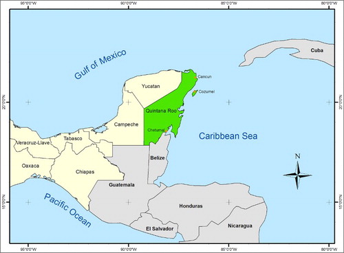
The area has a predominantly low relief, the climate is warm and humid with summer rains, with an average annual temperature of 27.6°C and an average annual rainfall of 1263.3 mm (CNA, 2016). It lies on a structure of tertiary sediments with some quaternary deposits, composed mainly of calcite, dolomite and small amounts of gypsum (Ordoñez & Garcia, 2010). There are few surface rivers, because most of the water moves underground, and there is an abundance of karstic depressions such as sinkholes, uvalas and cenotes. The most common soil groups are Leptosols, Phaeozems, Vertisols and Gleysols, and the vegetation is mainly medium and low tropical rainforest.

There are 23 natural protected areas that represent 25.3% of the surface in the study area (SINAP, 2016). The main economic activities are tourism and trade. Agricultural activity is focused in the south and occupies less than 20% of the surface of the State. Corn, sugar cane and timber are the main crops.

3. Methodology

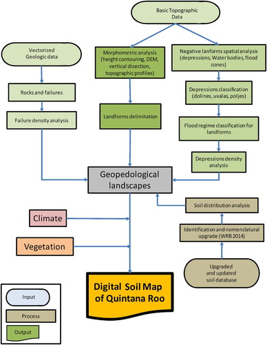
The development of the digital soil map consisted of three stages. The first two followed the geopedological approach, and the third incorporated other variables into the model to build and apply pedotransfer functions that relate soil characteristics to other variables (Figure 2).

Figure 2. Methodological diagram.

The first stage consisted of the geomorphometric and spatial analysis of field data at a scale of 1:50,000 to identify landforms and to map the distribution of limestone karst depressions and their flood types in the state (Fragoso-Servón, Bautista, Frausto, & Pereira, 2014).

The second stage entailed the development of a spatial distribution model of soils associated with previously identified landforms. This was done by adding georeferenced soil data to their respective landforms.

The soil database is a compilation of field and laboratory data from 412 field sampling points and derived from four different sources (Table 1). Using physical and chemical properties, soils were classified in accordance with the World Reference Base system (IUSS, 2007) and allocated to 14 major soil groups (MSG) (Table 1). The resulting attribute table was completed using the full data matrix built in the GIS spatially joining climate and vegetation data reported for the study area by INEGI (2005) and CONAFOR-SEMARNAT (2011), respectively, to previously identified landforms.

Table 1. Soils identified in Quintana Roo.

Source	No. of points	Soil groups identified
INEGI	91	Arenosols, Calcisols, Cambisols, Phaeozems, Histosols, Leptosols, Luvisols, Regosols, Solonchaks Nitisols, Vertisols, Gleysols, Fluvisols
CIGA-UNAM	79	Arenosols, Calcisols, Cambisols, Gleysols, Leptosols, Kastanozems, Phaeozems, Luvisols, Nitisols, Solonchaks, Vertisols
INIFAP	57	Gleysols, Leptosols, Luvisols, Phaeozems, Vertisols
UQRoo	185	Arenosols, Gleysols, Leptosols, Phaeozems, Solonchaks, Cambisols, Luvisols, Regosols, Nitisols, Vertisols

Note: Sources: INEGI (2008). CIGA-UNAM: Field work by Dr Francisco Bautista Zúñiga (coauthor). INIFAP: Field work by MC Gonzalo de Jesús Zapata Buenfil (coauthor). UQRoo: Field work by Dr Patricia Fragoso Servón (main author).

This produced two data subsets, one of them formed by all the 412 landforms fully qualified, including MSG, and the other one without the MSG information.

For the third stage, the second subset was fully quantified to assign MSG information to each landform as if we were using a pedotransference function to link MSG to the other variables. To achieve this goal, all landforms were classified, with all variables were used to form classes, except for the MSG information.

The classification algorithms were established using data subsets consisting of landforms for which soil information existed in addition to other variables. Trained algorithms were applied to the full data matrix. The full variable set and its domains are shown in Table 2.

Table 2. Variables and their domains.

Vertical dissection (VD)		Geology	Karstic form and types of flood		Climate	Vegetation	Soils (WRB)
Subhorizontal plain		Holocene Pleistocene. Pliocene Miocene Oligocene Eocene Paleocene Cretaceous	Sinkhole	Permanent	Aw0 Aw0(x’) Aw1 Aw1(x’) Aw2(x’)	Irrigated agriculture Temporary Agriculture Cultivated Forest Cultivated pasture Mangrove Palmar Tular Popal Savannah High Jungle subperennifolia Low Jungle subperennifolia Low jungle subcaducifolia Low torn Jungle subcaducifolia Medium jungle subcaducifolia Medium jungle subperennifolia	Gleysols Leptosols Luvisols. Phaeozems Vertisols Arenosols Regosols Hystosols Cambisols Nitisols Solonchaks Kastanozems Fluvisols Calcisols
Wavy Plain	Slightly dissected			Temporary
	Averagely dissected			Rarely
	Strongly dissected		Uvala	Permanent
Hilly Plain	Slightly dissected			Temporary
	Averagely dissected			Rarely
	Strongly dissected		Polje	Permanent
Hills	Slightly dissected			Temporary
	Averagely dissected			Rarely
	Strongly dissected		Karstic Density***Density of failures
Mountain	Slightly dissected

Landforms were clustered based on the similarity of the first five variables and their respective domains. A cluster analysis (CA), using the Gamma coefficient of Goodman–Kruskal as the metric algorithm was performed. This estimator is known as one of maximum similarity that is useful to handle large volumes of hierarchical data that match the order and the value (Nelson, 1986) (Equation (1)):(1) $\mathit{D}=\mathbf{1}-\left(\frac{{\mathit{N}}_{\mathit{s}}-{\mathit{N}}_{\mathit{d}}}{{\mathit{N}}_{\mathit{s}}+{\mathit{N}}_{\mathit{d}}}\right)$(1) where D is distance or similarity between the pairs of objects; N_s is the number of matching objects in attributes and sequence and N_d is the number of different objects on attributes and sequence. The linkage algorithm used was the weighted mean.

This clustering analysis was validated by three tests (Pseudo F, Pseudo-t test and consistency or distortion of Dunn) to verify that the results are that of greater likelihood:

1. A test of Pseudo F, provides the resulting tree and has a probability value for the node formed with regard to the probability of all nodes that make up the group; hence, it appears frequently as the null distribution in the variance analysis (Equation (2)).(2) $\mathit{F}=\left(\frac{{\mathit{U}}_1/{\mathit{d}}_1}{{\mathit{U}}_2/{\mathit{d}}_2}\right)$(2) where U₁ and U₂ follow a Chi-square distribution with d₁ and d₂ degrees of freedom and U₁ and U₂ which are statistically independent.

2. Pseudo-t test, which consists of the comparison of average distances and variances within and between groups, representing the dispersion of the nodes or density of the tree (Equation (3)).(3) $\mathit{t}=\frac{\overline{{\mathit{X}}_1}-\overline{{\mathit{X}}_2}}{{\mathit{s}}_{\overline{{\mathit{X}}_1}-\overline{{\mathit{X}}_2}}}$(3) where: $\overline{X_1}$ and $\overline{X_2}$ are intra and intergroup average distances and ${\mathit{s}}_{\overline{{\mathit{X}}_1}-\overline{{\mathit{X}}_2}}$ are differences of the variance with respect to the sizes of the groups.

3. Consistency or distortion of Dunn for the validity of the Grouping (Halkidi, Batistakis, & Vazirgiannis, 2002; Havens, Bezdek, Keller, & Popescu, 2008; Omran, Engelbrecht, & Salman, 2007) (Equation (4)).(4) $\mathit{D}=\frac{{\mathit{d}}_{\min }}{{\mathit{d}}_{\max }}$(4) where d_min is the minimum distance intergroup and d_max is the maximum distance intragroup.

The result of this analysis is a consistent model of the spatial distribution of soil, where data from a soil group were used to assign polygons to the corresponding group (MacMillan, 2004).

The next step is related to map validation and verification. The classes were verified by two types of statistical analysis: principal components analysis (PCA) and classification analysis (CA). The PCA identified the sources of data set variability and sorted them by importance (Jongman, Ter Braak, & van Tongeren, 1995).

The hierarchical model obtained from the PCA and the data matrix including soil data was used as input to estimate the uncertainty of the classification with the program WEKA (Hall et al., 2009). Four classifications using three different algorithms were performed:

• Classifications 1 and 2 were classifications using decision tables with simple and exhaustive search (Kohavi, 1995; Mukerjee, 2012);

• Classification 3 was a classification by construction of exceptions to the initial rule (RIDOR – Ripple-Down-Rules) (Gaines & Compton, 1995); and

• Classification 4 was a classification by partition rules (PART) (Frank & Witten, 1998).

The final map shows the spatial distribution of soils. This map was verified for consistency and accuracy against soil and environmental field data.

4. Results

The first clustering identified 869 entities of identical units by their attributes. To keep uncertainty as low as possible, 85% of similarity was chosen as the threshold value, resulting in 188 groups that depicted various environmental conditions. This clustering was validated by three tests: Pseudo F, Pseudo-t and the distortion coefficient of Dunn.

Pedological information was spatially joined to the groups formed by the CA to predict what soil types are likely to be found in each of the polygons in relation to the rest of the attributes, thus establishing a pedotransfer function that depicts the relationship between soil and the other attributes for each polygon. Where more than one soil group is assigned to a polygon, only the first three most probable soil groups are depicted on the map.

Sixty-five groups with no soil data are found in 103 polygons, representing 0.6% of the total number of polygons and occupying only 0.2% of the state area.

To identify and sort the sources of variability in the data set, a principal component analysis (PCA) was performed, defining the variables that have greater weight in the relationship between soils and attributes depending on the set of similarities of the classes formed (Table 3).

Table 3. Principal components analysis loadings.

No.	Component	Value	Percentage of variance explained	Cumulative percentage
1	VD and Karstic form	5.32	19.0	19
2	Karstic Density	4.27	15.3	34
3	Density of failures	2.70	9.6	44
4	Flood	2.00	7.2	51
5	Climate	1.63	5.8	57
6	Water bodies	1.26	4.5	61
7	Age of rocks	1.04	3.7	65

A chi-square test of the PCA results gave a value of zero, indicating that the eigenvectors of the variables in the data matrix are not equal or independent, thus demonstrating the relationship that exists between the soil-forming factors that were considered in the analysis and the allocation of the soil types to the map polygons.

The PCA shows seven variables that have the greatest influence on the distribution of soils. This can be seen in Figure 3, where the inflection point separates the most important factors from the other variables in the dataset.

Figure 3. Scree graph of contribution to the variance.

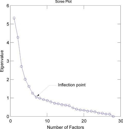
Considering the individual variances and their contribution to the total variance of the system, the analysis shows that vertical dissection (VD) and karstic forms contribute the most to the total system variance (19.0% and 15.3%, respectively) and explain 34.3% of the variation observed in the distribution of soils (Table 3). Following these two variables, karst and fault densities, and the flooding regime for karstic depressions, form a second variable group which along with the first group explain 51% of the variation.

The next group of components is formed by climate followed by the presence of either temporary or permanent bodies of water, and finally geology (age of parental materials). These three variables account for 14% of the variability of the distribution of soils. Together, these seven factors explain approximately 65% of the observed distribution of soils in the state.

Results from the analysis of classification (Table 4) show that more than 83% of soil type assignments are consistent and that polygons were correctly classified with the selected set of attributes once assigned to its corresponding soil type.

Table 4. Confusion analysis results.

Method	No. of polygons examined	No. of rules	Polygons correctly classified	Polygons incorrectly classified
Decision table of simple search	16,353	1119	83.26%	16.74%
Decision table of exhaustive search	15,353	1119	83.26%	16.74%
Exceptions (ripple-down-rules)	16,456	357,007	84.19%	15.81%
Partition rules (PART)	16,456	389	85.69%	14.31%

The differences between the three algorithms in terms of uncertainty (incorrectly classified polygons) are insignificant (2.43%). However, analysis of the respective confusion matrices shows that the PART algorithm has the maximum reduction in uncertainty.

Comparing the relative weight of the seven variables provided, and using PCA and the results of two non-supervised assessments of subsets of the seven variables used, it was found that three complex factors have greater weight in the distribution of soils: landforms (the VD and karstic forms), climate (rainfall and flooding) and geohydrology (lithology and surface hydrology).

The relationships between the variables used in the analyses define the relative importance of various factors on soil formation and allow the prediction of the type or types of soil that can be found at any point within the state (pedotransfer function). Current data allow the compilation of the map with about 14% to 16% uncertainty, which is probably a result of data precision and suggests the need for more control points to refine the model.

In the 14 identified soil groups (Table 5), the group that occupies the largest part of the territory is Leptosols (48.5%) followed by Gleysols and Phaeozems. These three together occupy 75.6% of the State’s surface (Figure 4). Soil groups that together account for less than 1% of the surface are Calcisols, Kastanozems, Regosols and Fluvisols.

Figure 4. Area occupied by principal soil groups in Quintana Roo.

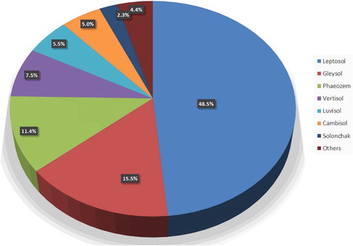
Table 5. Principal reference soil groups in Quintana Roo.

Principal reference soil group	No. polygons	Area (ha)	%
Leptosol (LP)	7376	2,452,346.72	48.47
Gleysol (GL)	3386	782,927.46	15.47
Phaeozem (PH)	1306	575,975.61	11.38
Vertisol (VR)	707	377,514.63	7.46
Luvisol (LV)	813	278,484.66	5.50
Cambisol (CM)	616	255,075.29	5.04
Solonchak (SC)	291	114,348.10	2.26
Histosol (HS)	17	63,380.86	1.25
Arenosol (AR)	622	52,623.73	1.04
Nitisol (NT)	184	45,745.75	0.90
Calcisol (CL)	23	11,689.65	0.23
Kastanozem (KS)	75	7329.12	0.14
Regosol (RG)	35	1701.35	0.03
Fluvisol (FL)	5	266.53	0.01
No data	103	10,767.20	0.21
Water bodies	897	29,194.10	0.58
Total	16,456	5,059,370.81	100.00

Each polygon is dominated by a group of soils that occupy the greatest area, with other groups of soils make up smaller proportions (Table 6). This situation is very frequent in Quintana Roo, where there are different groups of soils in small areas. To qualify the polygons and to build the map and its legend, only the three soils that occupy the largest area of the polygon were considered, resulting in 112 possible combinations of soils. The representation of these combinations and the database that accompanies it constitute the digital map of soils of Quintana Roo, at 50 m pixel resolution (Main Map).

Table 6. Principal and associated soil groups (see Table 5 for soil group symbol).

Principal RSG	Associated soil groups
LP	PH	LV	RG	VR	SC	NT	GL	HS	AR
GL	LP	LV	RG	VR	SC	PH	HS	AR
LV	LP	PH	GL	VR	SC	NT	CM
AR	LP	GL	RG	HS	SC	CM
PH	LP	LV	GL	VR	CM
KS	LP	LV	PH	VR	NT
VR	LP	LV	GL	PH
CM	LP	LV	PH	HS
SC	LP	GL	KS	AR
HS	LP	SC	RG
FL	LP	LV	PH
NT
RG

Note: RSG = Reference soil group.

5. Conclusions

A digital soil map of Quintana Roo was compiled at 50 m pixel resolution using a geomorphopedological approach to produce a map that reflects a synoptic view of the geomorphology, environmental conditions and associated soils.

This approach allows a thorough synthesis of environmental information of the components (climate, vegetation, soil) and geomorphological landscapes (including VD, geomorphometrics of the karst, faults and geology). Using various statistical models (cluster, principal component and classification analysis), the distribution pattern of soils in the territory was obtained.

The map shows a very high heterogeneity of soils in the studied area linked to geomorphometric heterogeneity not described in studies conducted before 2010 and earlier.

The methods used enabled the production of a map with a relatively low uncertainty. These methods are more useful for large-scale land management and decision-making than those currently in use in México.

The map was compiled with data from soil-forming factors and uses mathematical methods to infer information for the places where there are no data thus defining a pedotransfer function.

This research provides a new methodological framework that can be applied in other places and at different scales.

Due to its digital form, the whole database and the corresponding map are easily updatable at reduced costs at any scale equal or lower to the 50 m pixel resolution.

The methodology used allows the attainment of relatively low uncertainties for regional planning.

Software

The map was produced using Esri ArcGIS^® to build and manage the databases. Statistical analysis (clustering and PCA) were performed using SYSTAT^® v13 and classification analysis was carried out using WEKA^®. The final map was produced in ArcGIS^® and exported to PDF format.

Acknowledgements

We wish to thank the Statewide Program of Action on Climate Change of Quintana Roo for its support in the field work and the UQROO-FOMIX-2012 Project for granting permission to use the computing equipment for statistical analysis.

Disclosure statement

No potential conflict of interest was reported by the author.

ORCID

Patricia Fragoso-Servón http://orcid.org/0000-0003-0863-7156

References

- Behrens, T., & Scholten, T. (2006). Digital soil mapping in Germany – a review. Journal of Plant Nutrition and Soil Science, 169, 434–443. doi: 10.1002/jpln.200521962
- Brevik, E. C., Baumgarten, A., Calzolari, C., Jordán, A., Kabala, C., Miller, B. A., & Pereira, P. (2016). Editorial: Historical perspectives and future needs in soil mapping, classification, and pedologic modeling. Geoderma, 264, 253–255. doi: 10.1016/j.geoderma.2015.09.022
- Calzolari, C., & Filippi, N. (2016). Evolution of key concepts in modern pedology with reference to Italian soil survey history. Geoderma, 264, 275–283. doi: 10.1016/j.geoderma.2015.08.024
- Carré, F., McBratney, A. B., Mayr, T., & Montanarella, L. (2007). Digital soil assessments: Beyond DSM. Geoderma, 142, 69–79. doi: 10.1016/j.geoderma.2007.08.015
- CNA. (2016). Normales Climatológicas [WWW document]. Retrieved July 10, 2016, from http://smn1.conagua.gob.mx/index.php?option=com_content&view=article&id=42&Itemid=75
- CONAFOR-SEMARNAT. (2011). Inventario nacional forestal. . México: Comision Nacional Forestal, Secretaría del Medio Ambiente y Recursos Naturales.
- Fragoso-Servón, P., Bautista, F., Frausto, O., & Pereira, A. (2014). Caracterización de depresiones kársticas (tamaño, forma y densidad) a escala 1:50000 y sus tipos de inundación en el estado de Quintana Roo, México. Revista Mexicana de Ciencias Geológicas, 31, 127–137.
- Frank, E., & Witten, I. H. (1998). Generating accurate rule sets without global optimization. In Machine Learning: Proceedings of the fifteenth International Conference (pp. 144–151). Morgan Kaufmann.
- Gaines, B. R., & Compton, P. (1995). Induction of ripple-down rules applied to modeling large databases.
- Grunwald, S., Thompson, J. A., & Boettinger, J. L. (2011). Digital soil mapping and modeling at continental scales: Finding solutions for global issues. Soil Science Society of America Journal, 75, 1201. doi: 10.2136/sssaj2011.0025
- Halkidi, M., Batistakis, Y., & Vazirgiannis, M. (2002). Clustering validity checking methods: Part II. ACM Sigmod Rec., 31, 19–27. doi: 10.1145/601858.601862
- Hall, M., Frank, E., Holmes, G., Pfahringer, B., Reutemann, P., & Witten, I. (2009). The WEKA data mining software: An update. ACM SIGKDD Explorations Newsletter, 11(1), 10. doi: 10.1145/1656274.1656278
- Hartemink, A. E., Hempel, J., Lagacherie, P., McBratney, A., McKenzie, N., MacMillan, R. A., … Zhang, G.-L. (2010). Globalsoilmap.net – a new digital soil map of the world. In J. L. Boettinger, D. W. Howell, A. C. Moore, A. E. Hartemink, & S. Kienast-Brown (Eds.), Digital soil mapping (pp. 423–428). Dordrecht: Springer.
- Hartemink, A. E., & Minasny, B. (2014). Toward digital soil morphometrics. Geoderma, 230–231, 305–317. doi: 10.1016/j.geoderma.2014.03.008
- Havens, T. C., Bezdek, J. C., Keller, J. M., & Popescu, M. (2008). Dunn’s cluster validity index as a contrast measure of VAT images. Pattern Recognition, 2008. ICPR 2008. 19th International conference on, IEEE, Tampa, Florida, USA, pp. 1–4.
- INEGI. (2005). Carta de climas para a República Mexicana, 1:1000000. México: Instituto Nacional de Estadística Geografía e Informática.
- INEGI. (2008). Conjunto de datos de perfiles de suelos escala 1:250000. Serie II (Continuo Nacional). México: Instituto Nacional de Estadística Geografía e Informática.
- INEGI. (2016). Número de habitantes. Quintana Roo [WWW document]. Retrieved July 10, 2016, from http://cuentame.inegi.org.mx/monografias/informacion/QRoo/Poblacion/
- IUSS Working Group. (2007). World reference base for soil resources 2006, first update 2007 (World Soil Resources Reports No. 103). Rome: FAO.
- Jongman, R. H., Ter Braak, C. J., & van Tongeren, O. F. (1995). Data analysis in community and landscape ecology. Cambridge, UK: Cambridge University Press.
- Kempen, B., Brus, D. J., & de Vries, F. (2015). Digital operationalizing soil mapping for nationwide updating of the 1:50,000 soil map of the Netherlands. Geoderma, 241–242, 313–329. doi: 10.1016/j.geoderma.2014.11.030
- Kohavi, R. (1995). The power of decision tables. Proceedings of the European conference on machine learning. Berlin: Springer, pp. 174–189.
- Lagacherie, P. (2008). Digital soil mapping: To state-of-the-art. In Digital soil mapping with limited data (pp. 3–14). Dordrecht: Springer.
- MacMillan, R. B. (2004). Automated knowledge-based classification of landforms, soils and ecological spatial entities. Retrieved April 24, 2017, from https://www.reserchgate.net/profile/RaMacmillan/publication/301701700_Automated_knowledge-bassed_classification_of_landforms_soils_and_ecological_spatial_entities/links/5723f91708aee491cbe75.pdf
- McBratney, A., Mendonça Santos, M., & Minasny, B. (2003). On digital soil mapping. Geoderma, 117, 3–52. doi: 10.1016/S0016-7061(03)00223-4
- Miller, B. A., & Schaetzl, R. J. (2016). History of soil geography in the context of scale. Geoderma, 264, 284–300. doi: 10.1016/j.geoderma.2015.08.041
- Minasny, B., & McBratney, A. B. (2016). Digital soil mapping: A brief history and some lessons. Geoderma, 264, 301–311. doi: 10.1016/j.geoderma.2015.07.017
- Montanarella, L., Pennock, D. J., McKenzie, N. J., Badraoui, M., Chude, V., Baptista, I., … Vargas, R. (2015). The world’s soils are under threat. SOIL Discussions, 2, 1263–1272. doi: 10.5194/soild-2-1263-2015
- Mukerjee, P. (2012). Classification & association rule generation. In Data mining using WEKA. Kharagpur: Vinod Gupta School of Management, IIT Kharagpur.
- Nelson, T. O. (1986). BASIC programs for computation of the goodman-kruskal gamma coefficient. Bulletin of the Psychonomic Society, 24, 281–283. doi: 10.3758/BF03330141
- Omran, M. G., Engelbrecht, A. P., & Salman, A. (2007). An overview of clustering methods. Intell. Data in the Analisys Area., 11, 583–605.
- Ordoñez, I., & Garcia, M. (2010). Formas kársticas comunes de los cenotes del Estado de Quintana Roo (Mexico). Medioambiente, 9, 15–35.
- Sanchez, P. A., Ahamed, S., Carré, F., Hartemink, A. E., Hempel, J., Huising, J., … Mendonça-Santos, M. D. L. (2009). Digital soil map of the world. Science, 325, 680–681. doi: 10.1126/science.1175084
- SINAP. (2016). The National System of Protected Areas (SINAP) | National Commission of Natural Protected Areas | Government | gob.mx [WWW document]. Retrieved January 9, 2016, from http://www.gob.mx/conanp/acciones-y-programas/sistema-nacional-de-areas-protegidas-sinap
- Zinck, J. A. (1988). Physiography and soils, lecture notes Sol.4.1. Enschede: International Institute for Geoinformation Science and earth Observation (ITC). 156 p.
- Zinck, J. A. (2012). Geopedology, ITC special lecture notes series. Enschede: Faculty of Geo-Information Science and Earth Observation. 123 p.