Glacial geomorphology of the south Swedish uplands – focus on the spatial distribution of hummock tracts

ABSTRACT

We present the first comprehensive glacial-landform map of the south Swedish uplands (SSU), deglaciated 15–13 ka ago, using one consistent method and dataset; a Light Detection and Ranging-derived digital elevation model. In particular, this map focuses on the spatial distribution of hummock tracts. The distribution of hummock tracts reinforces previous thinking of a broad lobate east–west zone of hummocks across the southern part of the SSU. But this map also reveals a pattern of hummock tracts confined in what we call hummock corridors that have a radial pattern sub-parallel to the overall ice-flow direction. Hummocks occur in a wide variety of morphologies, but we also show the distribution of two distinct forms: V-shaped hummocks and ‘ribbed moraine’. Cross-cutting relationships between hummocks and glacial lineations indicate a more complex chronology than previously suggested. In places, lineations are overlain by hummocks and in other places hummocks are overlain by lineations. Additionally, directional variation of glacial lineations together with a complex end-moraine pattern suggests a dynamic ice sheet with multiple small lobes. Finally, mapped end moraines help to better correlate the deglacial timescales of western and eastern Sweden.

KEYWORDS:

• Glacial geomorphology
• hummocks
• southern Sweden
• deglaciation
• paleo-glaciology

1. Introduction

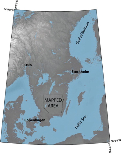
The glacial geomorphology of the south Swedish uplands (SSU; Figure 1) has been studied for over 100 years. However, a complete glacial-landform map has never been produced using a uniform dataset for the entire SSU (loosely defined as the area above 250 m a.s.l. in southern Sweden). The map presented here (Main Map) covers the SSU in the Swedish province of Småland but also extends into lower lying areas in the southern part of the mapped region (Figure 1). Until recently, mapping of glacial landforms has relied on the interpretation of topographic maps, aerial photographs or satellite images combined with field work. In areas with dense forest, photos and satellite images have not been optimal for creating detailed glacial geomorphologic maps. The SSU is one of these regions, and the production of a national 2-meter resolution elevation model (NH), based on Light Detection and Ranging (LiDAR), has revealed the landscape at an unprecedented level of detail (Lantmäteriet, 2015).

Figure 1. Overview map. Northeastern Europe with the mapped area in a black dotted box. Elevation data derived from the GEBCO dataset, GEBCO_2014 Grid, version 20150318, www.gebco.net.

This new dataset of the Swedish landscape allows scientists to produce and provide the best geomorphic maps and databases to date. Regional glacial geomorphological databases are important for both societal and academic use:

• They provide a more detailed view of glacial landforms that in turn allow for a better understanding and reconstruction of the glacial history.

• Better geomorphic maps provide a more accurate distribution of glacial features for the development of ice-sheet computer models, which are necessary for global climate models (Napieralski et al., 2007; Van Tatenhove, Van Der Meer, & Huybrechts, 1995).

• New LiDAR-based maps better reveal the landforms resulting from subglacial meltwater drainage, and this is crucial for the understanding of contemporary ice-sheet dynamics and meltwater processes.

• They can contribute to mineral exploration by yielding information on ice-flow directions (Klassen, 1999).

• They provide a way to accurately delineate groundwater recharge zones (e.g. eskers, deltas) and as input to hydrogeological models (Klint, Nilsson, Troldborg, & Jakobsen, 2013; Nilsson, Klint, Troldborg, & Jakobsen, 2011).

• These data are critical for land-use planning and as input in slope stability and surface deposits modeling (Daniels & Thunholm, 2014; Tryggvason, Melchiorre, & Johansson, 2014).

• Finally, these maps and databases illustrate our natural history in the form of maps to be used in education and for parks and reserves (Soyez, 1971).

Finally, this map, and the data collected during this work, acts as base data for ongoing research focused primarily on the hummock tracts of this region and their implication for glacial dynamics of the Fennoscandian Ice Sheet. We refer to a ‘hummock tract’ as a region of undulating, irregular knobby forms. The individual hill or knob is called a ‘hummock’ and a region characterized by many of these is called a ‘hummock tract’ In that sense, the term is intended to be parallel to terms like ‘dune field’ and ‘drumlin swarm’.

1.1. Regional geology and long-term geomorphic development

The bedrock in the area consists of Precambrian crystalline bedrock and is divided into two provinces. The western gneiss-dominated area lies within the Sveconorvegian province, and the eastern granite and porphyry-dominated area lies within the Transscandinavian Igneous Belt (Wik et al., 2009). The boundary between these two provinces runs roughly north–south passing west of Växjö.

A warm and humid climate in the Mesozoic Era deeply weathered exposed bedrock (Elvhage & Lidmar-Bergström, 1987). The region was uplifted during the late Oligocene and early Miocene epoch, and this rise formed what is now the south Swedish Dome (roughly coinciding with the SSU and also the area mapped within this study) (Lidmar-Bergström & Näslund, 2002). In Neogene time, this region was again uplifted, tilted and eroded forming the South Småland Peneplain (the western and southern parts of the study area) (Olvmo, Lidmar-Bergström, Ericson, & Bonow, 2005).

Regionally, peneplanation and deep weathering of the Precambrian bedrock have been the main processes developing the physiography of the SSU prior to Pleistocene glaciation. Subsequently, glacial and glaciofluvial processes during the Pleistocene have acted mainly as agents for removing weathered material. Nonetheless, glacial processes have significantly impacted the landscape, and glacial landforms are ubiquitous in the SSU.

During the Pleistocene, multiple ice sheets waxed and waned over the landscape in southern Sweden. Although records in Norway and on the continent reveal that the SSU must have been glaciated numerous times during the Pleistocene (Kleman, Stroeven, & Lundqvist, 2008; Sejrup et al., 2000), much of the record has been removed. Older till from these previous glaciations have been found in only a few places in southern Sweden (e.g. Hillefors, 1974; Miller, 1977; Påsse, 1998). Except for localities with till-covered stratified sediments (mostly sands), most of the glacial sediment in the SSU is from the late-Weichselian deglaciation (Möller & Murray, 2015).

The southernmost part of the mapped area became ice free at about 15 ka, and the SSU was completely ice free at about 13 ka (Anjar et al., 2014; Hughes, Gyllencreutz, Lohne, Mangerud, & Svendsen, 2015; Stroeven et al., 2016). In the mapped area, ice retreat took place above the highest shoreline so the ice margin retreated in a terrestrial environment (although there was calving in some local ice-dammed lakes (Nilsson, 1968). During deglaciation, there were several still-stands or re-advances of the ice margin (Agrell, Friberg, & Oppgården, 1976; Lundqvist & Wohlfarth, 2001); however, prominent, regional end moraines have not been identified in the SSU, except for the Vimmerby Moraine in the northeastern part of the mapped area (Figures 4(A) and 8) (Agrell et al., 1976; Johnsen, Alexanderson, Fabel, & Freeman, 2009; Stroeven et al., 2016).

1.2. Previous work

The earliest geological mapping in the region occurred during the late nineteenth century in a series of combined bedrock geology and surficial deposit surveys conducted in the field by the Geological Survey of Sweden (Blomberg, 1879, 1880; Holst, 1879, 1885, 1893; Hummel, 1877a, 1877b, 1877c; Stolpe, 1892). A large portion of this region was remapped for surficial deposits during the late twentieth and early twenty-first centuries (Geological Survey of Sweden, 2016).

Quaternary research during the latter half of the twentieth century in the SSU has covered a wide range of topics. However, three themes have emerged.

First, several studies have centered on specific landforms in the SSU, including hummocks, ribbed moraine, glaciofluvial canyons and streamlined bedforms. The hummocks and ribbed moraine were first discussed by Gavelin and Munthe (1907) and Stolpe (1911). The same landforms were later described by Bergdahl (1953) and Johnsson (1956) and mapped at small scale by Persson (1972). These studies revealed a broad zone of hummocks in a band primarily parallel to the former ice front, 20 to 40 km wide in the southern part of the SSU extending across southern Sweden and possibly temporally and geomorphically connected to the Göteborg Moraine (Möller, 1987; Möller & Dowling, 2015). The ribbed moraine areas in southern Småland were studied in great detail by Möller (1987, 2010) who proposed them to be landforms resulting primarily from the melting of stagnant, debris-rich ice stacked by thrusting within the ice due to a frozen toe. Subsequent subglacial and supraglacial melt-out of debris was followed by sediment gravity flows resulting in a sequence of melt-out and flow till.

Steep-sided canyon-like valleys carved into bedrock have been shown to have a large concentration in three parts of Sweden, one is within the mapped area (Olvmo, 1992) and he suggested these to be formed by subaerial glaciofluvial processes. Streamlined bedforms were mapped using a LiDAR-derived elevation model in this area for the statistical analysis of their shape compared to other regions by Dowling, Spagnolo, and Möller (2015). The results demonstrated that the southern Swedish streamlined bedforms are similar in morphology to their counterparts in the British Isles.

Second, regional stratigraphy has been a focus of study. There are many localities where fine-grained, sandy sediments occur below Weichselian till. Some of these localities were first described in connection with the early mapping activities (Fredholm, 1875; Hummel, 1877a). These sediment sequences are (1) the result of an oscillation during the last deglaciation, as first proposed by an amateur geologist named Strandmark (Möller & Murray, 2015; and references therein), or (2) they are older sediments overridden during the late-Weichselian advance (Rydström, 1971). Recent studies, using the OSL technique, show that it is likely that these sediments are from the mid-Weichselian or possibly deposited subglacialy during late-Weichselian (Alexanderson, 2010; Möller & Murray, 2015). However, the data used to estimate the age are complex and yield ambiguous age assignments (Alexanderson & Murray, 2007, 2012). Other than these buried sand units, there is no mention of older units due to their apparent absence from the region.

Third, several papers have been dedicated to identifying and dating ice-margin positions that were formed during deglaciation (Anjar et al., 2014; Johnsen et al., 2009; Lundqvist & Wohlfarth, 2001). The chronology of deglaciation in southern Sweden has been studied using surface exposure dating and suggests a steady deglaciation rate, from ice-free areas in southern Sweden at 16.1 ± 0.9 ka, The southern part of the mapped area was ice free at about 15 ka and the northern part by 13.8 ± 0.8 ka (Anjar et al., 2014). Clearly defined ice margins are barely present in the area, except for the lobate Vimmerby Moraine in the northeast (Figure 4(A)) (Agrell et al., 1976). The Vimmerby Moraine has been dated with surface exposure dating to 14.4 ± 0.9 ka (Johnsen et al., 2009). However, recent LiDAR mapping of ice-marginal landforms over southern Sweden reveals several end moraines, including a possible extension of the Berghem Moraine of western Sweden (Stroeven et al., 2016).

2. Data collection and methodology

For this report, landforms were mapped manually using ESRI ArcGIS® ArcMap™ 10.2 on a LiDAR-based digital elevation model (DEM) together with hillshade (45°, 310° and 270°) and slope rasters derived from the NH. The LiDAR DEM provides a ‘bare earth’ view of the landscape with a vertical resolution of 0.25 m and a horizontal pixel size of 2 m (Lantmäteriet, 2015). Mapping was conducted on a Wacom® CINTIQ® 27″ digital drawing table. Every part of the mapped area was screened twice at two different scales (1:15,000 and 1:60,000) in order to ensure recognition of landforms of different sizes. The digital data from surficial geology maps (Geological Survey of Sweden, 2016) and orthorectified aerial photographs of the area were used to assist with interpretations. Map design was carried out in Adobe® Illustrator® CS6.

3. Landform definitions and descriptions

The landform definitions used here are based on the descriptions of the Geological Survey of Sweden’s glacial geomorphologic map units (Peterson & Smith, 2013). However, some adjustments have been made, and some landform units have been added to fit the purpose of this map more accurately. The landforms are presented here in order from oldest to youngest. However, relative ages are not always constant throughout the mapped area and many landforms were likely made time-transgressively.

3.1. Glacial lineations

We use the term ‘glacial lineations’ to refer to subglacial landforms that are elongated in the direction of ice movement. All types of glacial lineations (e.g. drumlins, megaflutes, megascale glacial lineations, crag-and-tails) have been mapped and grouped together into two categories, drumlinoids and crag-and-tails. A crag-and-tail is mapped based on the visible presence of bedrock or other obstruction at the ice-proximal end of the landform. The category drumlinoids includes all other glacial lineations and streamlined bedforms regardless of genesis; drumlins, megaflutes and megascale glacial lineations.

3.2. Hummock tracts

Much of the SSU contains hummock tracts. Hummocks, like those found in these tracts, are commonly interpreted to have been formed by the collapse of supraglacial debris that overlies stagnant ice. However, similar landforms in other locations have been suggested to have formed in a variety of ways, involving subglacial, englacial, supraglacial and even proglacial processes (see Johnson & Clayton, 2003). Nonetheless, most of these hummocks have been routinely mapped in Sweden and elsewhere as ‘stagnation moraine’ or ‘dead-ice moraine’, which implies collapse from dead ice. But the large variation in morphology of these hummocky landforms, in, for example, the SSU and elsewhere, indicates that this landform class is heterogeneous, and this variability may indicate a variation in genesis as well.

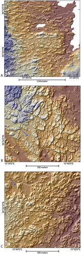
The vast majority of hummocks in the SSU found in the tracts consist of disorganized irregular hills and depressions, and it is this group of undifferentiated landforms that makes up the majority of the hummocks in the hummock tracts (Figure 2(C)). The undifferentiated tracts hold a large variation within the group in shape, size and relief, but the variation is not regionally consistent enough for a distinct classification without further study. However, we distinguish two special types with a significantly distinct morphology to map separately from the undifferentiated hummocks (Figure 2). First, there are semi-ordered systems of ridges transverse to ice flow, which were referred to initially as ‘Åsnen moraine’ by Möller (1987) but bear a strong morphologic similarity to ribbed moraine described elsewhere (Dunlop & Clark, 2006; Hättestrand & Kleman, 1999; Lundqvist, 1969, 1989; Möller, 1987) (Figure 2(A)). These ‘ribbed moraine’ or ‘Åsnen’ tracts grade into more irregular hummocks, and even though they are clearly more ridge-like than irregular, we consider them to be hummocks in the broad sense. We have chosen to refer to them as ‘ribbed moraine’. However, clearly defined ribbed moraine (i.e. Figures 2(A) and 5(C)) is rare in relation to the vast areas of other hummocks and is common only in the southern part of the mapped area (Möller, 2010). Second, there are hummocks that have a V-shaped appearance with apices pointed generally down-ice. These hummocks have gentle upice and steep down-ice slope. To our knowledge, these landforms have never been mapped before. However, similar landforms have also been newly discovered in Finland and reported on by Mäkinen, Kajuutti, Palmu, Ojala, and Ahokangas (2017) (Figure 2(B)).

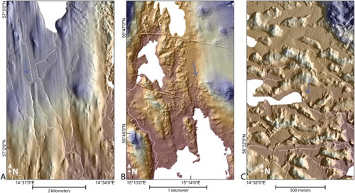
Figure 2. Examples of the variety within the hummock tracts. (A) Semi-ordered ridges transverse to ice flow. (B) V-shaped hummocks. (C) Disorganized irregular hills and depressions. Blue arrows display ice-flow direction from glacial lineations. Background: Hillshade (illumination from 315°) image overlying a colored DEM; brown = low elevation, grey = intermediate, purple = high.

Collectively, hummock tracts are mapped regardless of genesis and are used as a group name for any area that contains any type of non-bedrock hillock or mound with a round to elongate form in a chaotic to semi-ordered pattern. However, areas that specifically hold an abundance of ribbed moraine or V-shaped landforms are indicated on the map. The possible multiple origins of the various types of hummocks in the hummock tracts is the focus of ongoing field work and will be reported on in future papers.

3.3. Corridor margins

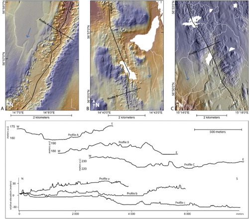
The category ‘corridor margins’ is used to define areas of hummock tracts that are observed in distinct radial zones or corridors, which we refer to as ‘hummock corridors’ (Figure 3). The majority of these areas are approximately parallel to the former ice-flow direction. In places, the hummock corridors occur as valleys in the landscape (Figure 3(A)). Elsewhere, they form linear zones of hummocks and other landforms with positive relief (Figure 3(B)). In a few localities, these corridors can be traced by merely scattered hummocks in areas with extensive bedrock outcrops (Figure 3(C)).

Figure 3. Examples of hummock tracts in corridors with cross profiles A–C and long profiles a–c. (A) Corridor incised into the surrounding streamlined surface. (B) Corridor with a generally positive relief. (C) Corridor marked by scattered hummocks and bedrock topography. Blue arrows display ice-flow direction from glacial lineations. Background: Hillshade image (illumination from 315° on (A) and (B), 90° on (C)) overlying a colored DEM; brown = low elevation, grey = intermediate, purple = high.

3.4. Eskers

Eskers are formed subglacially in tunnels and consist mainly of sorted sand and gravel. They often appear as sinuous ridges and on the map area they have discontinuous lengths of up to hundreds of kilometers and heights of tens of meters.

3.5. End moraines

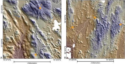
End moraines are ridges formed at the terminus of the ice sheet and demarcate a former stillstand or re-advance. Most moraines in the study area are distinct and stand out clearly from the surrounding terrain (Figure 4(A)). However, in areas dominated by hummock tracts, moraines are generally not as distinct as elsewhere. Rather, they are sub-continuous ridges appearing amongst the surrounding hummocks (Figure 4(B)).

Figure 4. Example of moraines within the mapped area. (A) Part of the Vimmerby Moraine with a N–S direction. Note the different directions and cross-cutting relationships of glacial lineations outside and inside the moraine. (B) Sub-continuous moraine with a lobate shape in an E–W direction. Orange arrows mark moraines. Blue arrows display ice-flow direction from glacial lineations. Background: Hillshade image (illumination from 45°) overlying a colored DEM; brown = low elevation, grey = intermediate, purple = high.

3.6. Glaciofluvial deltas

Glaciofluvial deltas are landforms composed of sand and gravel that have been transported by glacial meltwater and deposited in standing water. Subsequent to deglaciation, the landforms have been separated from the original body of water by land uplift and/or lake-level lowering. Glaciofluvial deltas with distinct deltaic morphology and flat surfaces are mapped.

3.7. Glaciofluvial canyons

Steep-sided canyon-like valleys were interpreted by Olvmo (1992) to be of glaciofluvial origin due to their connection to glaciofluvial deposits. Olvmo (1992) referred to these as ‘glaciofluvial canyons’, and we have placed the canyons he mapped on our map.

3.8. Proglacial and marginal meltwater channels

When glacial meltwater flows along the ice margin, it may erode channels into the substrate, we call these ‘marginal meltwater channels’ and they indicate ice-margin positions. ‘Proglacial meltwater channels’ form in front of any glacier where meltwater has enough discharge to erode into the substrate. Within the mapped area, there are outwash surfaces with proglacial, braided channels. However, these are not included on the map and only prominent proglacial meltwater channels are mapped. Some of these channels may have been created by jökhulhlaups or outburst floods from ice-dammed lakes. For design purposes, these two landforms have been grouped on the map into the category ‘Proglacial and marginal meltwater channels’. In contrast to glaciofluvial canyons that are incised in bedrock, the proglacial and marginal meltwater channels are cut in sediment.

4. Results and discussion

More than 20,000 features were mapped in this study. Of this total, more than 17,800 ice-flow indicators were mapped as drumlinoids and crag-and-tails (Table 1). Furthermore, 1481 km of eskers and 310 km of end moraines (457 individual segments) were mapped. This provides a new glacial geomorphological map of the SSU based on a homogenous dataset and methodology (Main Map).

Table 1. More than 20,000 features where mapped. The sum and individual count of all mapped landforms are presented in this table.

	Features (n)	Length (km)	Area (km^2)
Progl. and marginal meltwater ch.	552	–	–
Moraines	457	310	–
Glacifluvial deltas	305	–	–
Eskers	3532	1481	–
Hummock tracts	213	–	6438
Hummock tracts, ribbed moraine	23	–	372
Corridor sides	260	–	–
Glacial lineations
Large crag-and-tails	3729	–	–
Small crag-and-tails	3185	–	–
Large drumlins/drumlinoids	3936	–	–
Small drumlins/drumlinoids	6995	–	–
Total	23,187

The overall picture of the mapped glacial lineations displays a radial pattern throughout the area. Glacial lineations occur in three distinct geomorphic settings within the studied area. First, most glacial lineations form broad streamlined till-covered uplands where they provide a clear contrast to areas of bedrock or hummock tracts (Figure 5(A)). In places these surfaces are bordered and even cut by hummock corridors indicating that the broad streamlined surfaces predate some hummock tracts. Second, streamlined lineations occur within hummock tracts, in some places overlain by hummock deposits (Figure 5(B)) implying a similar age relationship as above. Third, in a few places, faint glacial lineations are superposed on ribbed moraine, indicating that at least part of the ribbed moraine within was overridden by active ice (Figure 5(C)). For this paper, we are not able to firmly conclude the genesis of the ribbed moraine in the SSU. Utilizing thorough stratigraphic investigations of the landforms depicted (Figure 5(C)), Möller (Möller, 1987, 2010) proposed a formation by melting of stagnant, debris-rich ice, stacked by thrusting due to a frozen toe. However, ribbed moraine mapped elsewhere, morphologically similar to the ribbed moraine in the SSU, is commonly considered to have been formed subglacially, and it may be that these features in the SSU were made in the same way (Dunlop & Clark, 2006; Hättestrand & Kleman, 1999; Lundqvist, 1969, 1989).

Figure 5. Examples of landscape position of glacial lineations. (A) Glacially streamlined surface. (B) Streamlined landform overlain by hummocks. (C) Subtle streamlined landforms superposed on hummocks. Blue arrows display ice-flow direction from glacial lineations. Background: Hillshade image (illumination from 45° on (A), 315° on (B), 90° on (C)) overlying a colored DEM; brown = low elevation, grey = intermediate, purple = high.

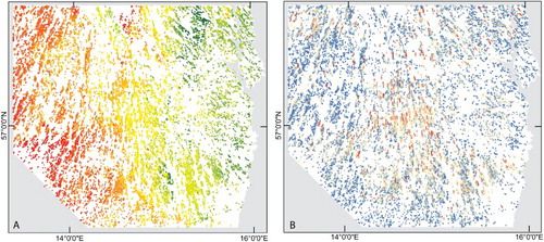
Glacial lineations trend toward the southwest in the western part of the mapped area and toward the southeast in the eastern part of the mapped area. Within this regional pattern, there are variations, often associated with moraines (Figure 6(A)). In places, there are smaller sets of lineations in a radial pattern, for example, the glacial lineations behind the Vimmerby Moraine (Figure 2(A)). However, a radial pattern is also apparent south of lake Vättern on the highlands to the east. Variations in direction of glacial lineations suggest a dynamically active ice sheet with multiple minor lobate ice-sheet margins. Further, glacial lineations display a range of lengths and features of similar dimensions occur in clusters (Figure 6(B)), which have been suggested to indicate variations in ice-flow velocity at the glacier bed (Stokes & Clark, 2002). This suggests that basal ice-flow velocity was highest in the central parts of the mapped area (Figure 6(B)).

Figure 6. Visualization of glacial lineation. (A) Glacial lineations colored by direction; green = westerly ice flow, yellow = southerly ice flow, red = easterly ice flow. (B) Glacial lineations colored by length; blue = short lineations, yellow = intermediate, red = long lineations.

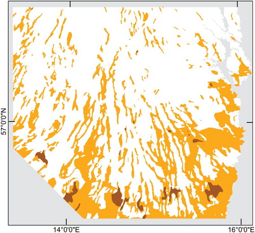
Hummock tracts cover 6438 km², approximately 30% of the mapped area, making it a typical landscape within the area, especially in the south. The areas of hummock tracts display an interesting pattern (Figure 7). First, there is the broad zone of hummock tracts in the southern part with an arcuate shape perpendicular to the former ice flow, and it is within this zone that ribbed moraine are present (Lundqvist & Wohlfarth, 2001; Möller, 2010; Persson, 1972). In places within this zone, ribbed moraines occur in ribbons and narrow tracts (Dunlop & Clark, 2006). Second, there are hummock tracts that are parallel to the overall ice flow, forming a radial pattern of elongate zones. It is these zones we refer to as hummock corridors. This radial pattern has never before been recognized on previous maps. Hummocks within these corridors generally can be described as disorganized irregular hills and depressions.

Figure 7. The mapped extent of hummock tracts display (undifferentiated = yellow, ribbed moraine = brown) a radial pattern parallel to the overall ice-flow direction.

In places, hummock corridors have vague lateral boundaries, but elsewhere they are quite distinct from the surrounding glacially streamlined surfaces. The width of these distinct corridors ranges from about 1 to 3 km. Some of them are clearly incised into the surrounding till surface and others are made up of positive forms (Figure 2).

The hummock corridors are often found in connection with eskers. The eskers that are mapped primarily follow the large corridors but also other valleys that trend from north to south. In other areas outside the valleys and corridors, eskers are small but can often be followed for long distances. A large number of the eskers in this region have been mined for sand and gravel and are more easily mapped on the LiDAR DEM as excavated hollows than ridge crests.

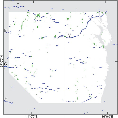
Until recently, only one significant moraine, the Vimmerby Moraine, has been reported in the SSU (Agrell et al., 1976). However, mapping on detailed DEMs has revealed many more moraines within the study area, and this has made it possible to connect the Vimmerby Moraine morphologically with the Berghem Moraine that enters the mapped area in the western part (Stroeven et al., 2016). Stroeven et al. (2016) reported that apart from a possible correlation of the Trollhättan Moraine with lobate moraines below and southeast of lake Vättern, no clear correlations between the southernmost west-coast moraines (i.e. Halland costal and Göteborg Moraines) are apparent. Their mapping efforts of moraines in the area show the absence of moraines within the central and southern part of the study area (Stroeven et al., 2016). Contrary to the findings of Stroeven et al. (2016), we present a series of end moraines within the central and southern parts of the mapped area, most of which appear within the hummock tracts. First, we find a continuation of the Gothenburg Moraine to the east of Lake Bolmen. Further to the east, short end-moraine fragments may also indicate other ridges formed at this time. Second, within the hummock tracts, we map a lobate moraine in the southeastern part of the study area. This ice margin becomes more pronounced if connected with glaciofluvial deltas and the abrupt end of several eskers (Figure 8). Third, we map a series of small moraines within the hummock tracts in the southwestern part of the mapped area.

Figure 8. End moraines (blue) and deltas (green) reflect former ice margins. Trollhättan Moraine (T) can be connected with a series of lobate moraines in its continuation. A connection between the Berghem Moraine (B) and Vimmerby Moraine (V) is noticeable. The Göteborg Moraine (G) can be extended to moraine fragments to the east. H = Halland coastal Moraines.

5. Conclusions

• This map is the first comprehensive inventory of glacial geomorphology, based on one method and one dataset, for this part of southern Sweden.

• The extent of hummock tracts in this region is not only, as previously shown, in the shape of a broad east–west zone in the southern part of the area, but also as hummocky corridors, which have a radial pattern, sub-parallel to the overall ice-flow direction in the area.

• Age relationships between hummocks and glacial lineations indicate both hummocks overlying glacial lineations and glacial lineations overlying hummocks. The latter indicates that some hummocks were either formed or overridden by active ice.

• The variation in the directions of ice-flow indicators and the shape of the end-moraine, suggests a dynamic ice sheet with multiple smaller lobate portions.

• Mapped end moraines yield more information about the connection of the eastern and western deglaciation timescale. Also, end moraines, interpreted as smaller ice lobe advances, are present north of the Vimmerby Moraine.

Software

ESRI ArcGIS® ArcMap™ 10.2 was used for mapping and Adobe® Illustrator® CS6 was used for map design.

Acknowledgements

Constructive comments from Jakob Heyman, Mats Olvmo and Liselott Wilin on an earlier version of this map improved the design and readability. Furthermore, we acknowledge Henrik Mikko and Carl-Henric Wahlgren for discussions on glacial geology and bedrock geology, respectively. Finally, we would like to thank Ola Fredin, Paul Dunlop and Thomas Pingel for insightful reviews that significantly improved this paper and map.

Disclosure statement

No potential conflict of interest was reported by the authors.

ORCID

Gustaf Peterson http://orcid.org/0000-0002-9537-283X

Mark D. Johnson http://orcid.org/0000-0003-0015-1514

Colby A. Smith http://orcid.org/0000-0002-7335-6281

Additional information

Funding

This work was funded by the Geological Survey of Sweden with additional funding from the Swedish Society for Anthropology and Geography.

References

- Agrell, H., Friberg, N., & Oppgården, R. (1976). The Vimmerby Line – An ice-marginal zone in north-eastern Småland. Meddelanden Från Lunds Universitets Geografiska Institution, Avhandlingar, 549, 71–91.
- Alexanderson, H. (2010). Sub-till glaciofluvial sediments at Hultsfred, South Swedish Upland. GFF, 132(3–4), 153–159. doi: 10.1080/11035897.2010.508134
- Alexanderson, H., & Murray, A. S. (2007). Was southern Sweden ice free at 19–25 ka, or were the post LGM glacifluvial sediments incompletely bleached? Quaternary Geochronology, 2(1–4), 229–236. doi: 10.1016/j.quageo.2006.05.007
- Alexanderson, H., & Murray, A. S. (2012). Problems and potential of OSL dating Weichselian and Holocene sediments in Sweden. Quaternary Science Reviews, 44, 37–50. doi: 10.1016/j.quascirev.2009.09.020
- Anjar, J., Larsen, N. K., Håkansson, L., Möller, P., Linge, H., Fabel, D., & Xu, S. (2014). A 10 Be-based reconstruction of the last deglaciation in southern Sweden. Boreas, 43(1), 132–148. doi: 10.1111/bor.12027
- Bergdahl, A. (1953). Israndbildningar i östra syd- och mellansverige med särskild hänsyn till åsarna. Meddelanden Från Lunds Universitets Geografiska Institution, Avhandlingar, 23, 208.
- Blomberg, A. (1879). Beskrifning till kartbladet Ölmestad. Sveriges Geologiska Undersökning, Serie Ab, 5.
- Blomberg, A. (1880). Beskrifning till kartbladet Nissafors. Sveriges Geologiska Undersökning, Serie Ab, 6.
- Daniels, J., & Thunholm, B. (2014). Rikstäckande jorddjupsmodell. Geological Survey of Sweden – Report, 14.
- Dowling, T. P. F., Spagnolo, M., & Möller, P. (2015). Morphometry and core type of streamlined bedforms in southern Sweden from high resolution LiDAR. Geomorphology, 236, 4–63. doi: 10.1016/j.geomorph.2015.02.018
- Dunlop, P., & Clark, C. D. (2006). The morphological characteristics of ribbed moraine. Quaternary Science Reviews, 25(13–14), 1668–1691. doi: 10.1016/j.quascirev.2006.01.002
- Elvhage, C., & Lidmar-Bergström, K. (1987). Some working hypotheses on the geomorphology of Sweden in the light of a new relief map. Geografiska Annaler, Series A: Physical Geography, 69(2), 343–358. doi: 10.2307/521194
- Fredholm, K. A. (1875). Några iakttagelser öfver skiktade gruslager bland krosstensgrus i Småland. Geologiska Föreningen I Stockholm Förhandlingar, 2(12), 522–525. doi: 10.1080/11035897509448101
- Gavelin, A., & Munthe, H. (1907). Beskrivning till kartbladet ‘Jönköping’. Geological Survey of Sweden – Serie Aa, 123.
- Geological Survey of Sweden. (2016). Surface deposits 1:25 – 100 K.
- Hättestrand, C., & Kleman, J. (1999). Ribbed moraine formation. Quaternary Science Reviews, 18(43–61). doi: 10.1016/S0277-3791(97)00094-2
- Hillefors, Å. (1974). The stratigraphy and genesis of the Dösebacka and Ellesbo. Geologiska Föreningen I Stockholm Förhandlingar, 96, 355–373. doi: 10.1080/11035897409454289
- Holst, N. O. (1879). Beskrifning till kartbladet ‘Lessebo’. Sveriges Geologiska Undersökning, Serie Ab, 4.
- Holst, N. O. (1885). Beskrifning till kartbladet ‘Hvetlanda’. Sveriges Geologiska Undersökning, Serie Ab, 8.
- Holst, N. O. (1893). Beskrifning till kartbladet ‘Lenhovda’. Sveriges Geologiska Undersökning, Serie Ab, 15.
- Hughes, A. L. C., Gyllencreutz, R., Lohne, Ø. S., Mangerud, J., & Svendsen, J. I. (2015). The last Eurasian ice sheets – A chronological database and time-slice reconstruction, DATED-1. Boreas, 45, 1–45. doi: 10.1111/bor.12142
- Hummel, D. (1877a). Beskrifning till kartbladet ‘Huseby’. Sveriges Geologiska Undersökning, Serie Ab, 1.
- Hummel, D. (1877b). Beskrifning till kartbladet ‘Ljungby’. Sveriges Geologiska Undersökning, Serie Ab, 2.
- Hummel, D. (1877c). Beskrifning till kartbladet ‘Vexiö’. Sveriges Geologiska Undersökning, Serie Ab, 3.
- Johnsen, T. F., Alexanderson, H., Fabel, D., & Freeman, S. P. H. T. (2009). New 10Be cosmogenic ages from the Vimmerby moraine confirm the timing of Scandinavian ice sheet deglaciation in Southern Sweden. Geografiska Annaler, 91(2), 113–120. doi: 10.1111/j.1468-0459.2009.00358.x
- Johnson, M. D., & Clayton, L. (2003). Supraglacial landsystems in lowland terrain. In D. J. A. Evans (Ed.), Glacial landsystems (pp. 228–258). London: Arnold.
- Johnsson, G. (1956). Glacialmorfologiska studier i södra Sverige. Avhandlingar: Meddelanden Från Lunds Universitets Geografiska Institution, 30, 407.
- Klassen, R. A. (1999). The application of glacial dispersal models to the interpretation of till geochemistry in Labrador, Canada. Journal of Geochemical Exploration, 67, 245–269. doi: 10.1016/S0375-6742(99)00080-1
- Kleman, J., Stroeven, A. P., & Lundqvist, J. (2008). Patterns of quaternary ice sheet erosion and deposition in Fennoscandia and a theoretical framework for explanation. Geomorphology, 97(1–2), 73–90. doi: 10.1016/j.geomorph.2007.02.049
- Klint, K., Nilsson, B., Troldborg, L., & Jakobsen, P. (2013). A poly morphological landform approach for hydrogeological applications in heterogeneous glacial sediments. Hydrogeology Journal, 21(6), 1247–1264. doi: 10.1007/s10040-013-1011-2
- Lantmäteriet. (2015). Produktbeskrivning: GSD-Höjddata, grid 2+ (Product description). Gävle.
- Lidmar-Bergström, K., & Näslund, J.-O. (2002). Landforms and uplift in Scandinavia. Geological Society, London, Special Publications, 196, 103–116. doi: 10.1144/GSL.SP.2002.196.01.07
- Lundqvist, J. (1969). Problems of the so-called Rogen moraine. Sveriges Geologiska Undersökning, C 648.
- Lundqvist, J. (1989). Rogen (ribbed) moraine – Identification and possible origin. Sedimentary Geology, 62, 281–292. doi: 10.1016/0037-0738(89)90119-X
- Lundqvist, J., & Wohlfarth, B. (2001). Timing and east–west correlation of south Swedish ice marginal lines during the Late Weichselian. Quaternary Science Reviews, 20(10), 1127–1148. doi: 10.1016/S0277-3791(00)00142-6
- Mäkinen, J., Kajuutti, K., Palmu, J., Ojala, A., & Ahokangas, E. (2017). Triangular-shaped landforms reveal subglacial drainage routes in SW Finland. Quaternary Science Reviews, 164, 37–53. doi: 10.1016/j.quascirev.2017.03.024
- Miller, U. (1977). Pleistocene deposits of the Alnarp Valley, southern Sweden – Microfossils and their stratigraphical application. Lundqua Thesis, 4, 125.
- Möller, P. (1987). Moraine morphology, till genesis, and deglaciation pattern in the Åsnen area, south-central Smaland, Sweden. Lundqua Thesis, 20, 146.
- Möller, P. (2010). Melt-out till and ribbed moraine formation, a case study from south Sweden. Sedimentary Geology, 232(3–4), 161–180. doi: 10.1016/j.sedgeo.2009.11.003
- Möller, P., & Dowling, T. P. F. (2015). The importance of thermal boundary transitions on glacial geomorphology; mapping of ribbed/hummocky moraine and streamlined terrain from LiDAR, over Småland, South Sweden. Gff, 137(4), 252–283. doi: 10.1080/11035897.2015.1051736
- Möller, P., & Murray, A. S. (2015). Drumlinised glaciofluvial and glaciolacustrine sediments on the Småland peneplain, South Sweden – New information on the growth and decay history of the Fennoscandian Ice Sheets during MIS 3. Quaternary Science Reviews, 122, 1–29. doi: 10.1016/j.quascirev.2015.04.025
- Napieralski, J., Hubbard, A., Li, Y., Harbor, J., Stroeven, A. P., Kleman, J., … Jansson, K. N. (2007). Towards a GIS assessment of numerical ice-sheet model performance using geomorphological data. Journal of Glaciology, 53(180), 71–83. doi: 10.3189/172756507781833884
- Nilsson, E. (1968). The late-quaternary history of Southern Sweden: Geochronology, ice-lakes, land-uplift. Kungliga svenska vetenskapsakademiens handlingar, Fjärde serien, 12(1), 1–117.
- Nilsson, B., Klint, K. E. S., Troldborg, L., & Jakobsen, P. R. (2011). A new approach for evaluating geological heterogeneity in areas covered with clay till using ‘The poly morphological concept’. Geological Society of America Abstracts with Programs, 43, 559.
- Olvmo, M. (1992). Glaciofluvial canyons and their relation to the Late Weichselian deglaciation in Fennoscandia. Zeitschrift Für Geomorphologie, 36(3), 343–363.
- Olvmo, M., Lidmar-Bergström, K., Ericson, K., & Bonow, J. M. (2005). Saprolite remnants as indicators of pre-glacial landform genesis in Southeast Sweden. Geografiska Annaler: Series A, Physical Geography, 87(3), 447–460. doi: 10.1111/j.0435-3676.2005.00270.x
- Påsse, T. (1998). Early Weichselian interstadial deposits within the drumlins at Skrea and Vinberg, southwestern Sweden. GFF, 120, 349–356. doi: 10.1080/11035899801204349
- Persson, T. (1972). Geomorphological studies in the South Swedish highlands with special reference to the glacial forms. Avhandlingar: Meddelanden Från Lunds Universitets Geografiska Institution, 66.
- Peterson, G., & Smith, C. A. (2013). Description of units in the geomorphic database of Sweden. SGU-Rapport, 4.
- Rydström, S. (1971). The Värend district during the last glaciation. Geologiska Föreningen I Stockholm Förhandlingar, 93(3), 537–552. doi: 10.1080/11035897109455384
- Sejrup, H. P., Larsen, E., Landvik, J., King, E. L., Ha, H., & Nesje, A. (2000). Quaternary glaciations in southern Fennoscandia: Evidence from southwestern Norway and the northern North Sea region. Quaternary Science Reviews, 19, 667–685. doi: 10.1016/S0277-3791(99)00016-5
- Soyez, D. (1971). Geomorfologisk kartering av nordvästra Dalarna för naturvårdssyften. Forskningsrapport Naturgeografiska Institutionen, Stockholms Universitet, 11.
- Stokes, C. R., & Clark, C. D. (2002). Are long subglacial bedforms indicative of fast ice flow? Boreas, 31, 239–249. doi: 10.1080/030094802760260355
- Stolpe, M. (1892). Beskrifning till kartbladet ‘Nydala’. Sveriges Geologiska Undersökning, Serie Ab, 14.
- Stolpe, P. (1911). En sydsvensk israndlinje och dess geografiska betydelse. Göteborgs Kungliga Vetenskaps Och Vitterhetssamhälles Handlingar, Fjärde Följden, XIII, 57.
- Stroeven, A. P., Hättestrand, C., Kleman, J., Heyman, J., Fabel, D., Fredin, O., … Jansson, K. N. (2016). Deglaciation of Fennoscandia. Quaternary Science Reviews, 147, 91–121. doi: 10.1016/j.quascirev.2015.09.016
- Tryggvason, A., Melchiorre, C., & Johansson, K. (2014). A fast and efficient algorithm to map prerequisites of landslides in sensitive clays based on detailed soil and topographical information. Computers & Geosciences, 75, 88–95. doi: 10.1016/j.cageo.2014.11.006
- Van Tatenhove, F. G. M., Van Der Meer, J. J. M., & Huybrechts, P. (1995). Glacial-geological/geomorphological research in west Greenland used to test an ice-sheet model. Quaternary Research, 44, 317–327. doi: 10.1006/qres.1995.1077
- Wik, N.-G., Claeson, D., Bergström, U., Hellström, F., Jelinek, C., Juhojuntti, N., … Wikman, H. (2009). Beskrivning till regional berggrundskarta över Kronobergs län. Sveriges Geologiska Undersökning, Serie K, 142, 1–68.