Seabed sediments (grain size) of Nordland VI, offshore north Norway

ABSTRACT

This paper presents a seabed sediments (grain size) map of the Nordland VI area (25,000 km²) off the Lofoten islands, north Norway. The map is based on multibeam echosounder data (bathymetry and backscatter), visual analysis of 215 video transects (each 700-m long), and visual and grain-size analysis of seabed sediment samples from 40 sampling stations acquired by grabs, boxcores and multicores. A total of 14 sediment classes were identified, with sediments varying in grain size from mud to boulders. Seabed types also include bedrock and bioclastic sediments from degrading cold-water coral reefs. The continental shelf is mostly characterised by coarse-grained sediments such as gravelly sand and sandy gravel, especially in till areas. In basins and glacial troughs, finer-grained sediments such as sandy mud and muddy sand dominate. The upper continental slope (300–600-m water depth) is characterised by coarse-grained sediments related to the influence of the strong north-east flowing Norwegian Atlantic Current. In deeper areas, finer-grained sediments are prominent. Below 1000-m depth, mostly mud and mud with sediment blocks occur.

KEYWORDS:

• Sediment grain size
• Norwegian Sea
• multibeam
• continental shelf
• continental slope
• Trænadjupet slide

1. Introduction

The Norwegian seabed mapping programme MAREANO (www.mareano.no) was launched in 2006 in order to improve the knowledge of the Norwegian seafloor. The programme performs detailed mapping of bathymetry and topography, seabed sediments, contaminants, biodiversity and biotopes. The Institute of Marine Research (IMR), the Geological Survey of Norway (NGU) and the Norwegian Mapping Authority (Norwegian Hydrographic Service, NHS) comprise the Executive Group responsible for carrying out the MAREANO field sampling, mapping and scientific studies. The knowledge gained from MAREANO provides input to ecosystem-based management, organised through integrated management plans covering the Norwegian offshore areas. MAREANO mapping includes the Seabed sediments (grain size) maps which form an important basis for biotope maps, and are used by management and industry for planning purposes.

More than 175,000 km² of the Norwegian continental shelf and slope, down to 3000-m depth, have been mapped since 2005. All results from the mapping programme are published on http://www.mareano.no/en/maps/mareano_en.html, including the following geological map products: Seabed sediments (grain size), Seabed sediments (genesis), Sedimentary environment, Landscapes and Landforms. To perform this mapping, MAREANO has acquired a suite of marine data sets such as multibeam bathymetry and backscatter, seabed sediment samples and cores, videos of the seafloor and high resolution sub-bottom profiler data which provide the basis for map production.

This paper focuses on one of the main products of the MAREANO programme, the Seabed sediments (grain size) map, made by NGU for presentation at scales of 1:100,000–1:250,000. Spatial grain-size distribution and composition of the seabed sediments is an important parameter for many users, including the fisheries and petroleum industries. Detailed knowledge of the spatial grain-size distribution of seabed sediments is also a prerequisite for successful biotope mapping and pollution studies.

The Nordland VI area described in this paper is located to the west of the Lofoten-Vesterålen islands, north Norway. The area is ecologically important, including one of the largest known live cold-water coral reefs in the world (Røstrevet, Fosså et al., 2005) and very important fishing grounds. This area has been prioritised in the integrated management plan for the Barents Sea and the sea areas off the Lofoten Islands (Anon., 2006) because of possible conflicts between human activities (fishing and oil industries) and vulnerable marine ecosystems.

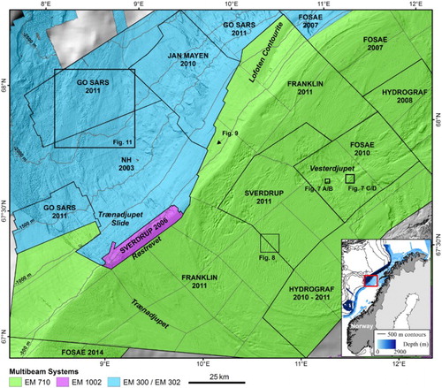
The Nordland VI area covers about 25,000 km² of the Norwegian continental shelf and slope, from 60 to 2700 m water depth (Figure 1). Here, the continental shelf (from the coast to about 300-m depth) was shaped by the Scandinavian ice sheet during the last glaciation, and is characterised by two prominent topographic features: the Trænadjupet Trough (about 480-m deep), and the Vesterdjupet Trough (about 290-m deep). The continental slope is incised by the large Trænadjupet Slide (Laberg & Vorren, 2000; Laberg, Vorren, Mienert, Bryn, & Lien, 2002), and numerous smaller slides, which have transported huge quantities of sediments towards deeper areas. Sediments are also transported along the continental slope by contour (parallel) currents. Sand and gravel waves locally occur on the upper slope, while finer-grained sediments accumulate between 600 and 1000 m water depth as a contourite deposit (Lofoten Contourite; Laberg, Vorren, & Knutsen, 1999). The upper slope south of the Trænadjupet Slide is characterised by glacigenic debris flows (Lingberg, Laberg, & Vorren, 2004). The same applies to the area between the Trænadjupet Slide in the southwest and the Lofoten Contourite in the north-east.

Figure 1. Map of Nordland VI showing the extent of multibeam echosounder surveys (outlined by black polygons), along with information on which research vessel (in capital letters) and year the different surveys were acquired. Also shown are geographic names and figure locations referred to in the text.

2. Methods

2.1. Data acquisition

The study area was mapped in 2003–2014 using four different multibeam echosounder systems (MBES) on seven different research vessels operated by five contractors (Figure 1 and Table 1). Two different MBES were used for less than 1000-m depth (EM1002: 95 kHz and EM710: 70–100 kHz range) and two for depths greater than 1000-m depth (EM300 and EM302, both 30 kHz). The specifications of the various MBES are listed in Table 2.

Table 1. Research vessel, operator, year of survey and multibeam echosounder system used during surveys.

Research vessel	Operator	Year	Multibeam echosounder
Unknown	Norsk Hydro	2003	EM300
Sverdrup	FFI	2006	EM1002
Sverdrup	FFI	2011	EM710
FOSAE	FUGRO	2007/2014	EM710 / EM300
Jan Mayen	University of Tromsø	2010	EM300
Hydrograf	Norwegian Mapping Authority	2010/2011	EM710
G.O. Sars	MAREANO	2011	EM302

Table 2. Technical specification of the different MBES used during surveys.

Multibeam echosounder	Frequency	Beamwidth	Beam numbers	Maximum ping rate	Swath coverage sector
EM710	70–100 kHz	0.5 × 1° to 2 × 2°	400/800	30 Hz	140°
EM1002	95 kHz	2 × 2°	111	>10 Hz	150°
EM300	30 kHz	1 × 1° to 2 × 4°	135	NA	150°
EM302	30 kHz	0.5 × 1° to 4 × 4°	144/288	NA	5.5 × depth

Note: NA: not applicable.

Both multibeam bathymetry and backscatter data were recorded (Figure 2). The multibeam backscatter corresponds to the seafloor acoustic reflectivity which is a measure of energy obtained from the echo intensity, which relates directly to the nature of the seafloor (Lurton & Lamarche, 2015). The bathymetry data were processed by NHS with CARIS and then gridded with QPS DMagic software, and the backscatter data were processed by NGU with two different softwares: Most of the FOSAE 2007 (multibeam data acquired by Fugro in 2007) and Hydrograf 2008 (multibeam data acquired by the Norwegian Mapping Authority in 2008) backscatter data (Figure 1) were processed with the Atlantic Geoscience Center (Geological Survey of Canada) Grass 5 software. Other backscatter data were processed by QPS FMGT software. An angle varying gain has been applied to the data to correct the angular dependence. The data density was sufficient for gridding at 5 m for depths <1000 m and 10–25 m for depths >1000 m, allowing detailed analysis of seabed features, especially on the continental shelf.

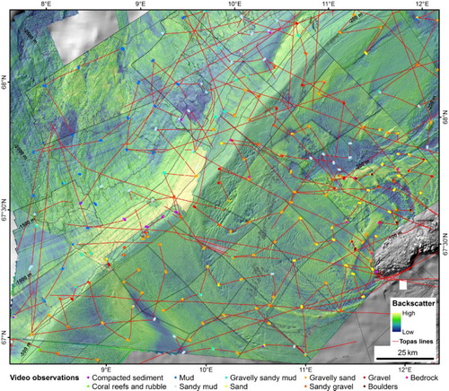
Figure 2. Backscatter data from the study area draped on a shaded relief image with depth contours labelled every 500 m. Coloured dots represent seabed sediment grain-size observations from video (only few observations are displayed along video lines due to the compressed scale of the figure) and red lines indicate locations of TOPAS seismic lines.

About 5500 km of high resolution seismic lines (Kongsberg TOPAS PS 018 parametric sub-bottom profiler, chirp modus, secondary beam frequency 0.5–6 kHz) with vertical resolution better than 1 m were also acquired. TOPAS lines were processed by the TOPAS software, and then converted to JPEG2000 by SegJp2 software (software courtesy of Geological Survey of Canada). Navigation shapefiles were extracted by SegJp2Viewer (software courtesy of Geological Survey of Canada) to be displayed in Esri ArcGIS. SegJp2Viewer was also used to display the lines.

Results from sampling of seabed sediments at 40 sampling stations are shown in Table 3. The samples were collected for biological, environmental and sedimentological studies by grab, boxcorer and multicorer. The sediment samples were first described visually onboard and then analysed later for spatial grain-size distribution. Fine-grained samples acquired with multicores were processed by NGU using Coulter Laser 200. Sandy and gravelly samples taken by grab and boxcorer were analysed by IMR using sieve or sieve and pipette analyses (Konert & Vandenberghe, 1997). The results were used to calibrate the visual video observations and for geochemistry and environmental studies.

Table 3. Sampling stations (Bx: boxcore, MC: multicore).

Station number	Depth (m)	Latitude	Longitude	Grab	Bx	MC	Seabed classification
R642	2352	68°15′39	09°15′12	x	x	x	Sandy mud
R646	2085	67°49′12	08°25′35	x	x	x	Mud/sandy mud
R653	1802	67°37′76	08°23′24	x			Gravelly sandy mud/gravelly muddy sand
R657	859	67°21′13	08°38′42	x	x		Gravelly muddy sand
R667	242	67°32′34	09°36′97	x	x		Sandy muddy gravel/sandy gravel, bioclastic sediments
R671	768	67°53′68	09°52′88	x			Sandy mud
R710	147	67°31′21	11°37′61	x			Fine sand
R721	181	67°50′87	11°48′55	x			Muddy sand/sand
R726	209	67°52′78	11°19′08	x	x	x	Sandy mud/muddy sand
R733	219	60°42′77	10°17′16	x			Unsuccessful
R736	245	67°51′11	10°22′03	x			Sand
R739	263	67°47′74	11°09′54	x			Sandy mud
R743	263	67°59′86	10°31′19	x	x		Gravelly muddy sand/gravelly sand
R749	1863	67°47′09	08°59′56	x	x		Sandy mud
R754	798	67°48′09	09°41′78	x	x		Gravelly muddy sand
R755	854	67°56′57	09°53′05	x	x		Gravelly sandy mud
R758	171	68°02′41	11°13′39	x	x		Gravelly muddy sand
R763	660	68°17′27	10°42′29	x	x		Gravelly muddy sand
R769	1964	68°20′84	10°04′29	x	x	x	Mud/sandy mud
R776	1021	68°11′32	10°21,71	x	x	x	Sandy mud / muddy sand
R782	1700	68°03,51	09°28′23	x	x	x	Mud/sandy mud
R786	1277	67°57′56	09°36′83	x	x	x	Mud
R793	175	67°40′36	10°46′74	x	x		Gravelly sand/sand
R805	172	67°41′82	11°31′44	x			Muddy sand
R809	145	67°29′81	11°12′70	x			Sand
R814	225	67°24′01	10°11 ′31	x			Sand
R818	918	67°35′72	09°12′24	x	x	x	Mud
R821	546	67°01′42	08°13′32	x	x		Gravelly sandy mud
R828	399	67°05′60	08°55′05	x	x		Gravelly muddy sand
R830	240	67°02′35	10°59′56	x			Gravelly sand
R838	380	67°07 ′66	09°55 ′64	x	x		Muddy sand
R841	202	67°12′22	10°27 ′47	x			Muddy sand
R844	182	67°16′62	11°31′94	x	x		Muddy sand
R848	182	67°13′22	10°55′17	x			Muddy sand
R849	188	67°24′24	10°49′29	x	x		Muddy sand/sand
R858	477	67°07′65	09°26′45	x	x		Sandy mud/muddy sand
R863	297	67°19′03	09°30′73	x	x		Gravelly sandy mud
R870	135	67°23′33	11°37′2	x			Sand
R877	2534	68°28′44	09°48′21	x	x	x	Sandy mud/mud
R879	1582	67°33′58	08°35′07	x	x	x	Mud
R882	1117	67°17′13	08°08′24	x	x	x	Mud/sandy mud

Video surveys were performed using IMR’s towed video platform CAMPOD (Buhl-Mortensen, Buhl-Mortensen, Dolan, Dannheim, & Kröger, 2009). All in all, 215 video transects of 700-m length were acquired in an area of about 25,000 km² (Figure 2). A preliminary interpretation of the seafloor sediments was done during the acquisition of the video transects utilising a custom built logging programme (CampodLogger). Fewer sediment classes were used during real time logging than in the final Seabed sediments (grain size) map. The description of the sediment grain-size classes follow the SOSI standard (a Norwegian national standard for geographical data), modified from Folk (1954) (English version (incomplete): Mardal, 2009; Norwegian version: https://objektkatalog.geonorge.no/Objekttype/Index/EAID_13D3A7C5_05FC_485e_A53D_935ABD6106CC) (Table 4). In addition to the grain-size classes, a few other classes (Table 4) are included in the Seabed sediments (grain size) map, for example, compacted sediments and bioclastic sediments. The results from the CampodLogger were output as text files, one per video transect. The text files were then compiled in Microsoft Excel files used to create point shapefiles. All available information was assembled and the map was interpreted and digitised using Esri ArcGIS. A detailed description of MAREANOs methods and products can be found at http://www.mareano.no/en/about_mareano/methods.

Table 4. SOSI code list for grain-size composition (modified from Folk, 1954).

Symbol	Grain size	Abbr.	Definition/description	SOSI code
	Mud	M	Clay:silt ratio from 1:2 to 2:1 and clay+silt >90%, sand <10%, gravel <2%	20
	Mud with sediment blocks	–	Mud alternating with blocks of hard sediments.	21
	Sandy mud	sM	Clay:silt ratio from 1:2 to 2:1 and clay+silt >50%, sand <50%, gravel <2%	40
	Muddy sand	mS	Sand >50%, clay:silt ratio from 1:2 to 2:1 and clay+silt <50%, gravel <2%	80
	Sand	S	Sand >90%, clay+silt <10%, gravel <2%	100
	Gravelly sandy mud	gsM	Sand:silt+clay ratio from 1:9 to 1:1, gravel 2–30%	115
	Gravelly muddy sand	gmS	Sand:silt+clay ratio from 1:1 to 9:1, gravel 2–30%	120
	Gravelly sand	gS	Sand:silt+clay ratio >9:1, gravel 2–30%	130
	Sandy gravel	sG	Sand:silt+clay ratio >9:1, gravel 30–80%	160
	Gravel, cobbles and boulders	GB	Dominant grain sizes are gravel, cobbles and boulders.	175
	Sand, gravel and cobbles	SGB	Sand, gravel, cobbles and boulders in frequent interchange.	185
	Compacted sediments or sedimentary rocks	–	Submarine outcrop of compacted sediments or sedimentary bedrock.	300
	Thin or discontinuous sediment cover on bedrock. Sediments with varying grain size	–	Lateral variation of small basins with sediments and exposed bedrock, and/or bedrock with thin/discontinuous sediment cover. Sediments in small basins may have varying grain size.	1
	Bioclastic sediments	–	Mud, sand and gravel of biological origin.	500

Note: The table contains only classes used in the Nordland VI area.

2.2. Map production

Backscatter, bathymetry and ground-truthing information from videos and sediment samples were used for interpreting the Seabed sediments (grain size) map (Main Map). The first studies of the effect of bottom type and bottom roughness on the backscatter started in the 1980s (e.g. De Moustier, 1986). In 2015, the Geohab backscatter working group published a report compiling the knowledge about backscatter and its link to the sediment characteristics showing, among other things, the importance of the backscatter data for sediment mapping (Lurton & Lamarche, 2015). Indeed, backscatter values give information about the bottom type and its physical characteristics. Scattering of the signal is controlled by the acoustic impedance (hardness or softness), the surficial roughness of the seafloor and the presence of heterogeneities on or immediately beneath the seabed surface including gas bubbles, shell fragment and living organisms (Lurton & Lamarche, 2015). For example, for a muddy or a homogeneous seabed, the signal is strongly attenuated and the backscatter values are low, whereas for a gravelly or a heterogeneous seabed the signal is strongly reflected and the backscatter values are high. Gas can also have a strong influence on the backscatter values. Fonseca, Mayer, Orange, and Driscoll (2002) observed a strong increase of the backscatter values (4–5 dB in this example) in water deeper than 100 m. Many other parameters such as the water column (e.g. water turbidity, salinity and temperature), the MBES frequency and the acquisition parameters also influence the backscatter signal. This means that multibeam surveys tend to have backscatter values which are consistent within each survey but not necessarily between surveys. Nevertheless, it is possible to adjust the backscatter mosaics to produce more uniform datasets (e.g. Hughes Clarke et al., 2008). Multibeam frequency is an important factor as it determines how deep the signal penetrates into the seabed, especially in soft sediments (Table 2). For instance, the EM300 system penetrates much deeper into the seabed than the higher frequency systems EM710 and EM1002. Thus, the backscatter signature may vary for a seabed that appears homogeneous in video data. In summary, backscatter strength does not provide a direct measure of sediment grain size but can be used to characterise the seabed, even if there are still strong dependencies on the angle and frequency of insonification (Weber and Lurton, in Lurton & Lamarche, 2015).

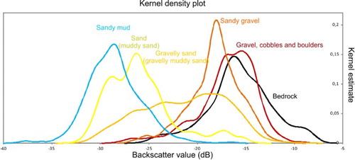
The first assumption for classifying the backscatter is that the backscatter values increase with grain size. This can be shown by using Kernel Density Estimation (KDE) (Parzen, 1962). In the example shown (Figure 3), the KDE of c. 6500 points from onboard interpretation of 28 video lines was plotted against backscatter values of two mosaics (Fosae 2010, see Figure 1 for location). Despite some positioning errors and sediment misinterpretations (e.g. the 30% gravel limit between gravelly sand and sandy gravel is not always easy to define visually), the backscatter values clearly increase from sandy mud to gravel, cobbles and boulders.

Figure 3. KDE plot of c. 6500 points from onboard interpretation of 28 video lines plotted against backscatter values of two mosaics (Fosae 2010, located in Figure 1).

The backscatter data were visually classified based on ground-truthing information (videos, grabs, boxcores, multicores, TOPAS) (Bellec et al., 2009). Each mosaic was classified individually with its own sediment class limit values. Both backscatter and ground-truthing data were symbolised in ArcGIS in a way promoting visual recognition of the spatial distribution of different sediment classes (Figures 4 and 5). This is done by defining backscatter intensity intervals based on ground-truthing information, which are assumed to broadly correspond to different sediment types, and by using the Symbology options in ArcGIS (Figure 5). This classified backscatter then needs to be interpreted in terms of sediment grain size. Multibeam bathymetry and its derivatives (e.g. slope) and landforms (e.g. moraines, pockmarks and sand waves) were also used for the interpretation. As different surveys can show different backscatter values, each survey was individually visually classified. The sediment classes were then manually digitised by integrating the backscatter values, the geomorphological features and the bathymetry derivatives (Table 5).

Figure 4. From backscatter to sediment map. Classified video observations are represented by coloured dots. (A) Backscatter map, (B) Backscatter classified based on sediment grain-size information from video observations and (C) Interpreted Seabed sediments (grain size) map.

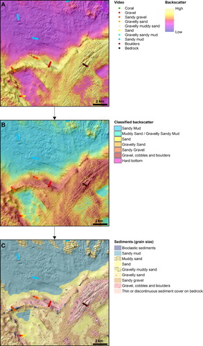
Figure 5. Example of backscatter classification in ArcGIS. Left panel: Layer properties in ArcGIS showing the options for ‘classified’; Right panel: Histogram and classes.

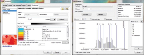
Table 5. Relationship between backscatter, relief and landforms used to guide sediment class interpretation.

		Relief
Sediment class	Backscatter	Low	High	Common landforms
Mud	Very low	x		Pockmarks
Mud with sediment blocks	Low – variable	x	x	Slide ridges and blocks
Sandy mud	Very low	x		Pockmarks
Muddy sand	Low	x		Flat seafloor, some pockmarks
Sand	Medium	x		Relatively flat seafloor, ripples on videos, occasional sandwaves
Gravelly sandy mud	Low to medium	xx	x	Rugged seafloor, smooth iceberg ploughmarks, pockmarks
Gravelly muddy sand	Medium to High	xx	x	Rugged seafloor, iceberg ploughmarks
Gravelly sand	High		x	Moraines, ridges, iceberg ploughmarks
Sandy gravel	High		x	Moraines, ridges, iceberg ploughmarks
Sand, gravel and cobbles	High		x	Moraines, ridges, iceberg ploughmarks
Gravel, cobbles and boulders	Very high		x	Relatively flat seafloor (in 5 m MBES grids) close to bedrock area or on slopes, iceberg ploughmarks
Bedrock	High – variable		x	Highly rugged seafloor
Compacted sediments	Variable		x	Slide escarpments in canyons and slope areas with slopes >15°, slide ridges and blocks
Bioclastic sediments	Variable	x	xx	Biogenic reefs

Note: Only objects and landforms larger than 100 m are mapped by MAREANO. An exception is biogenic reefs which are mapped even if they are smaller than 100 m across. x: common; xx: very common.

Sediment grain-size interpretations in the Seabed sediments (grain size) map (Main Map) represent approximately the uppermost 10 cm of the seabed. Fourteen sediment classes were used (Table 5, Figure 6). Three of these did not show a clear backscatter pattern and were instead mapped based on bathymetry data and its derivatives. These classes do not describe grain size, but rather sediment type: Bioclastic sediments, compacted sediments (compacted sediments or sedimentary rocks), and bedrock (thin or discontinuous sediment cover on bedrock, sediments with varying grain size). Bedrock generally shows a high backscatter response very similar to the gravel, cobbles and boulders class, and so cannot be distinguish by using the backscatter alone. However, it is very well-defined in the shaded relief map by showing a special pattern with high rugosity. Bioclastic sediments do not have a clear backscatter signature but are easily recognisable on the shaded relief map as they form mounds (Figure 7, see details below). Compacted sediments were interpreted along steep canyon walls or slide scars where videos showed this sediment type and where slopes were steeper than 15° measured in a 50 × 50 m grid. Compacted sediments can be found under the soft surface layer of the Norwegian continental shelf and slope. In some areas, the upper soft layer does not occur, mostly due to erosion, and the compacted sediments are then outcropping.

Figure 6. Examples of video observations for different sediment classes. 10 cm between red laser dots.

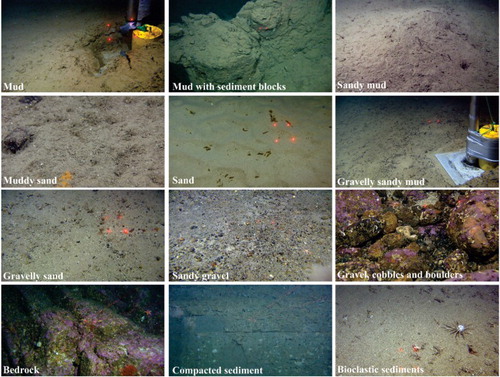
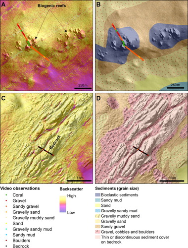
Figure 7. Examples of how bioclastic sediments and bedrock (thin or discontinuous sediment cover on bedrock) are interpreted from shaded relief and backscatter data. (A) Backscatter mosaic on shaded relief showing biogenic reefs, (B) interpreted sediment grain-size map showing bioclastic sediments, (C) backscatter mosaic on shaded relief in bedrock area, (D) interpreted sediment grain-size map showing bedrock and other sediment types. The video class ‘Coral’ includes both live corals and bioclastic sediments (sediments consisting of dead coral structures ranging in grain size from sand to blocks, and remnants of other dead organisms). See Figure 1 for location.

One of the classes was created for deep areas with slide scars: Mud with sediment blocks. Videos from these areas show a cover of mud, TOPAS data show that the mud thickness varies from zero to a few meters, while backscatter mosaics show strong variability in reflectivity. EM300/EM302 MBES signals used to map these areas penetrate deep into the seabed due to their low frequency and do not necessarily reflect the sediment composition in the uppermost c. 10 cm of the seabed that we intend to map. The variability of the signals is interpreted as related to slide blocks and sediments lying very close to the surface and sometimes outcropping. Two main sediment classes were used for the continental slope: mud, and mud with sediment blocks.

3. Results

3.1. Continental shelf

The continental shelf is characterised by large areas of coarse sediments (gravelly sand, sandy gravel, and sand, gravel and cobbles) especially in shallow shelf areas where till has been ploughed by icebergs. Shallow depressions are largely covered by sand and gravelly muddy sand, whereas deeper basins (e.g. Vesterdjupet and the Trænadjupet glacial trough) are characterised by finer sediments (sandy mud and muddy sand). Moraines are usually composed of coarser sediments, whereas sediments in depressions between the moraines consist mainly of finer-grained sediments (sand) (Figure 8). Rims (ridges) of iceberg ploughmarks are also often characterised by a higher content of gravel, cobbles and boulders on the seabed surface.

Figure 8. Moraines (ridges) showing high backscatter (relatively coarser sediments) separated by lower backscatter areas (relatively soft sediments, sand). See Figure 1 for location.

Precambrian crystalline bedrock occurs along the coastline, southeast of Vesterdjupet (Figure 7(C,D)) and north of Vesterdjupet (see Figure 1 for location). Bedrock areas (thin or discontinuous sediment cover on bedrock) are often surrounded by coarse sediments (gravel, cobbles and boulders).

Bioclastic sediments (Figure 7(A,B)) are a common sediment type in Nordland VI. The sediment type is interpreted on and around biogenic reefs. The sediment class is predominantly present along the northern side of Trænadjupet and at Røstrevet (Røst Reef) (see Figure 1 for location).

3.2. Upper continental slope

The upper continental slope occurs at about 300–1000-m water depth. It is characterised by slide scars, slide deposits and glacigenic debris flows which have transported coarse sediments to the deep areas. The c. 4000 years old Trænadjupet Slide affected an area of about 14,000 km² with a run-out distance of about 200 km (Laberg & Vorren, 2000; Laberg et al., 2002). The upper headwall of the slide scar is about 40-km long, and extends up to 2 km into the outer part of the shelf, thus cutting the outermost part of the Trænadjupet palaeo-ice stream drainage system (Ottesen, Dowdeswell, & Rise, 2005). It is up to 150-m high, and commonly very steep with slope angles above 25° (www.mareano.no).

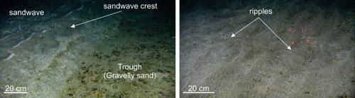
The uppermost part of the slope between about 300 and 700 m depth is characterised by coarse sediments (gravelly sand, sandy gravel, and gravel, cobbles and boulders). The North Atlantic Current locally exceeds 100 cm/s west of the Lofoten and Vesterålen islands (Andersson, Orvik, LaCasce, Koszalka, & Mauritzen, 2011), with a slope current showing mean values of 0.2–0.4 m/s (Heathershaw, Hall, & Huthnance, 1998). This strong current effectively prevents deposition of mud. Ripples and other current related bedforms are common at 400–500-m depth (Figure 9).

Figure 9. Sandwaves and sand ripples at 550 m water depth. See Figure 1 for location.

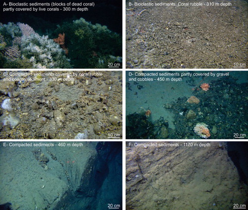
Bioclastic sediments occur around cold-water coral reefs on slide ridges and slide blocks consisting of compacted sediments (Thorsnes, Rise, Bellec, & Chand, 2016). Compacted sediments in the Trænadjupet Slide scar are often partly covered by sandy gravel, gravel, cobbles and boulders, and bioclastic sediments (Figure 10).

Figure 10. Examples of bioclastic sediments and compacted sediments between 300 and 1170-m depth.

Below 600–700 m water depth, sediments become finer grained and gravelly sandy mud and gravelly muddy sand cover most of the seafloor, including compacted sediments and glacigenic debris flows. Sandy mud occurs in channels and depressions. Farther north, the Lofoten Contourite (Laberg et al., 1999) is characterised by sandy mud.

3.3. Below 1000-m depth

Hemipelagic sediments and deposits from the Trænadjupet Slide dominate below about 1000 m water depth. The slide deposits are partly covered by hemipelagic sediments, commonly less than one meter thick.

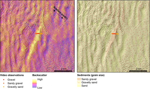
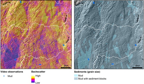
Below 1000-m depth, EM300/302 backscatter data (Figure 11) show strongly variable intensities whereas video observations indicate a quite homogeneous seafloor. Low backscatter areas are interpreted as basins with deposition of hemipelagic mud. Areas of medium to high backscatter are interpreted as slide deposits with a cover of hemipelagic sediments of variable thickness, classified as mud with sediment blocks.

Figure 11. Example of backscatter data and interpreted sediment map at about 2000-m depth. See Figure 1 for location.

4. Conclusions

This paper presents the Seabed sediments (grain size) map for the Nordland VI management area west of the Lofoten-Vesterålen islands, which covers about 25,000 km² offshore north Norway. The paper also details methods used for data collection and interpretation. Fourteen different seabed and sediment classes have been utilised.

The continental shelf (c. 100–300 m water depth) is characterised by large areas of coarse sediments, mainly gravelly sand, sandy gravel, and sand, gravel and cobbles. These sediments mostly occur on moraines and where till has been ploughed by icebergs. Fine-grained sediments (sandy mud and muddy sand) occur in deeper basins on the shelf (e.g. Vesterdjupet) and in the Trænadjupet Trough. Shallower areas are often covered by sand and gravelly muddy sand. There are also several bedrock outcrops along the coast and on the outer shelf. Bioclastic sediments, mostly comprising remains of living cold-water coral reefs, are particularly abundant along the northern margin of Trænadjupet and at Røstrevet.

The uppermost slope (300–700-m depth) is marked by the huge Trænadjupet Slide scar and numerous glacigenic debris flows. Coarse sediments (mainly gravelly sand, sandy gravel and gravel, cobbles and boulders) dominate. Bioclastic sediments occur at the live Røstrevet and on slide blocks in the Trænadjupet Slide scar. Sandwaves, sand ripples and other current related bedforms are common down to 400–500-m depth due to the strong Norwegian Atlantic Current. Below 700-m depth, the sediments become finer grained (mostly gravelly sandy mud and gravelly muddy sand). Compacted sediments occur in the Trænadjupet Slide area, both in slide escarpments and in slide blocks and ridges.

Below 1000-m depth, the seabed is mostly covered by fine-grained sediments (mud, mud with sediment blocks and sandy mud). Slide blocks are partly covered by fine-grained hemipelagic sediments.

Software

The bathymetry data were processed in CARIS HIPS and SIPS hydrographic software by NHS and gridded in QPS DMagic software.

The backscatter data were processed by NGU with two different software: AGC (Grass 5) software from the Geological Survey of Canada and QPS FMGT software.

Sediments and geological features were identified and digitised on-screen using Esri ArcGIS.

TOPAS data were processed with TOPAS software from Kongsberg. Processed TOPAS files were converted to JPG2000 with SegyJp2 software and displayed with SegyJp2viewer, both from the Geological Survey of Canada.

Data

The grain-size interpretations are stored in NGU’s Marine Geological Database (Oracle). Formatted PDF maps have been created for printouts and illustrations.

Grain-size data and maps are available for viewing http://www.mareano.no/en/maps/mareano_en.html and downloading http://www.mareano.no/en/download-data/the-geological-survey-of-norway-ngu (digital data, WMS-layer, pdf).

Acknowledgements

We acknowledge all participants of the MAREANO programme (www.mareano.no) for their input to this paper. The multibeam data were acquired and supplied by NHS. The data are released under a Creative Commons Attribution 4.0 Internationel (CC BY 4.0): https://creativecommons.org/licenses/by/4.0/.

Disclosure statement

No potential conflict of interest was reported by the authors.

References

- Andersson, M., Orvik, K. A., LaCasce, J. H., Koszalka, I., & Mauritzen, C. (2011). Variability of the Norwegian Atlantic Current and associated eddy field from surface drifters. Journal of Geophysical Research, 116, 433. doi: 10.1029/2011JC007078
- Anon. (2006). Report No. 8 to the Storting (2005–2006) integrated management of the marine environment of the Barents Sea and the sea areas off the Lofoten islands. Oslo: Ministry of Environment.
- Bellec, V. K., Dolan, M. F. J., Bøe, R., Thorsnes, T., Rise, L., Buhl-Mortensen, L., & Buhl-Mortensen, P. (2009). Sediment distribution and seabed processes in the Troms II area – offshore North Norway. Norwegian Journal of Geology, 89, 29–40.
- Buhl-Mortensen, P. B., Buhl-Mortensen, L., Dolan, M., Dannheim, J., & Kröger, K. (2009). Megafaunal diversity associated with marine landscapes of northern Norway: A preliminary assessment. Norwegian Journal of Geology, 89, 163–171.
- De Moustier, C. (1986). Beyond bathymetry: Mapping acoustic backscattering from the deep seafloor with Sea Beam. The Journal of the Acoustical Society of America, 79(2), 316–331. doi: 10.1121/1.393570
- Folk, R. L. (1954). The distinction between grain size and mineral composition in sedimentary rock nomenclature. The Journal of Geology, 62(4), 344–359. doi: 10.1086/626171
- Fonseca, L., Mayer, L. A., Orange, D., & Driscoll, N. (2002). The high-frequency backscattering angular response of gassy sediments: Model/data comparison from the Eel River Margin, California. The Journal of the Acoustical Society of America, 111(6), 2621–2631. doi: 10.1121/1.1471911
- Fosså, J. H., Mortensen, L. B., Christensen, O., Lundälv, T., Svellingen, I., Mortensen, P. B., & Alvsvåg, J. (2005). Mapping of Lophelia reefs in Norway: Experiences and survey methods. In A. Freiwald & J. M. Roberts (Eds.), Coldwater corals and ecosystems (pp. 359–391). Berlin: Springer.
- Heathershaw, A. D., Hall, P., & Huthnance, J. M. (1998). Measurements of the slope current, tidal characteristics and variability West of Vestfjorden, Norway. Continental Shelf Research, 18, 1419–1453. doi: 10.1016/S0278-4343(98)00051-X
- Hughes Clarke, J. E., Iwanowska, K. K., Parrott, R., Duffy, G., Lamplugh, M., & Griffinn, J. (2008). Inter-calibrating multi-source, multi-platform back scatter data sets to assist in compiling regional sediment type maps: Bay of Fundy. Paper presented at the proceedings of the Canadian hydrographic conference and national surveyors (2008), pp. 2–8.
- Konert, M., & Vandenberghe, J. (1997). Comparison of laser grain size analysis with pipette and sieve analysis: A solution for the underestimation of the clay fraction. Sedimentology, 44, 523–535. doi: 10.1046/j.1365-3091.1997.d01-38.x
- Laberg, J. S., Vorren, T., & Knutsen, S.-M. (1999). The Lofoten Contourite Drift off Norway. Marine Geology, 159, 1–6. doi: 10.1016/S0025-3227(98)00198-4
- Laberg, J. S., & Vorren, T. O. (2000). The Trænadjupet Slide, offshore Norway – morphology, evacuation and triggering mechanisms. Marine Geology, 171, 95–114. doi: 10.1016/S0025-3227(00)00112-2
- Laberg, J. S., Vorren, T. O., Mienert, J., Bryn, P., & Lien, R. (2002). The Trænadjupet Slide: A large slope failure affecting the continental margin of Norway 4000 years ago. Geo-Marine Letters, 22, 19–24. doi: 10.1007/s00367-002-0092-z
- Lingberg, B., Laberg, J. S., & Vorren, T. O. (2004). The Nyk Slide – morphology, progression, and age of a partly buried submarine slide offshore northern Norway. Marine Geology, 213, 277–289. doi: 10.1016/j.margeo.2004.10.010
- Lurton, X., & Lamarche, G. (Eds.) (2015). Backscatter measurements by seafloor-mapping sonars. Guidelines and Recommendations. 200p. Retrieved from http://geohab.org/wp-content/uploads/2014/05/BSWGREPORT-MAY2015.pdf
- Mardal, G. (2009). Superficial geology, English version – SOSI standard 4.0. Report of Norwegian mapping Authority, June 2009, 38 p.
- Ottesen, D., Dowdeswell, J. A., & Rise, L. (2005). Submarine landforms and the reconstruction of fast-flowing ice streams within a large Quaternary ice sheet: The 2500-km long Norwegian-Svalbard margin. Geological Society of America Bulletin, 117, 1033–1050. doi: 10.1130/B25577.1
- Parzen, E. (1962). On estimation of a probability density function and mode. The Annals of Mathematical Statistics, 33(3), 1065–1076. doi: 10.1214/aoms/1177704472
- Thorsnes, T., Rise, L., Bellec, V. K., & Chand, S. (2016). Shelf-edge slope failure and reef development: Trænadjupet Slide, mid-Norwegian shelf. In J.A. Dowdeswell, M. Canals, M. Jakobsson, B. J. Todd, E. K., Dowdeswell, & K. A. Hogan (Eds.), Atlas of submarine glacial landforms: Modern, Quaternary and ancient (pp. 413–414). London: Geological Society.