Visualisation of the influence of habitat on lichen occurrence, Toruń, Poland

ABSTRACT

The main aim of the paper was a visual comparison of lichen distribution with urban environmental factors. This paper presents a cartographic method for representing the spatial distribution of anthropogenic and natural factors in atmospheric air pollution and prevalent elements of the natural environment and their correlation to occurrences of two selected lichen species – the acidophilous Hypogymnia physodes and the nitrophilous Xanthoria parietina in the area of Toruń (Central Poland). Lichens are a good indicator of changes in habitat conditions. Analyses of the occurrence of lichens in Toruń were conducted for data covering a period of more than 60 years. A choropleth map method (a square tile grid map) was used, based on a grid of 144 one-kilometre squares (ATPOL). An inventory of taxa was made in 137 squares (localities). This recorded the type of substrate and abundance (extent) of occurrence.

KEYWORDS:

• Choropleth map – square tile grid map
• anthropopressure
• lichens
• urban ecology
• the city of Toruń
• Poland

1. Introduction

Lichens are a good bio-indicator of changes in habitat conditions, including in urban areas (Conti & Cecchetti, 2001; Davies, Bates, Bell, James, & Purvis, 2007; Lodha, 2013; Munzi et al., 2014). Lichens (Fungi lichenisati) are a group of fungi with a specific nutritional strategy which consists of absorbing carbon from autotrophic algae cells. This is a little ecosystem in which a dynamic balance is created between the fungus and the alga, and any change in habitat conditions can disturb this balance (Nash III 2009). Lichens are used in environmental monitoring all over the world (cf. inter alia, Estrabou, Filippini, Soria, Schelotto, & Rodriguez, 2011).

Cleveland (1993) presents descriptions of visualisation tools, and Robbins (2005) provides an introduction into ways to convey data correctly and cognitively. Different approaches to data analysis are presented, both statistical and visual. Beside the presentation of statistical data in tabular form, another presentation method is graphical. Friendly (2008) assumes two main methods – statistical charts and thematic cartography. Statistical charts and maps do not replace statistical tables, and this is not their purpose, but they are useful in simplifying the presentation of statistical data in a logical way and making the information more readily accessible to readers. This is the direct result of people’s perceptual ability to absorb data holistically and to register the relationships between individual graphical elements which are not noticeable when presented in tabular form, thus improving communicative effectiveness.

Using computer techniques such as GIS, it is possible to discover the influence of habitat conditions on the occurrence of individual species of lichen (cf. Ulshöfer & Rosner, 2001). Besides using a spatial approach to unambiguously identify the location of a particular phenomenon, using GIS and IT techniques also make it possible to show interdependent elements.

The method, which is based on one variation of a choropleth map – a square tile grid map – is simple and clear (Bertin, 1981; Cleveland, 1993; MacEachren & Taylor, 1994; O’Brien & Cheshire, 2016) because the method allows characteristics of the presented environment to be averaged and, with that, helps in interpreting the influence of abiotic conditions on the occurrence of biota of lichen. Unlike the point method, choosing the cartogram method made it possible to physically distribute the gathered data evenly.

Reference fields (basic fields, the reference unit, the statistical unit) are the key element of a cartogram in determining the level of detail of the data to be presented. The reference field in this method is most usually administrative units, river basins, divisions into geographical regions, or geometric basic fields, such as squares, rectangles, etc. Using geometric fields of a uniform shape and size make the areas presented on the map fully comparable (Robinson, Morrison, Muehrcke, Kimerling, & Guptill, 1995).

Meanwhile, using GIS techniques such as choropleth maps ensure the ability to conduct comparative analyses for other urban areas and to create databases based on habitat conditions (cf. Haberlie, Ashley, & Pingel, 2015). Researcher such as Cleveland (1993) used gridded maps. It is possible to visualise information about the geographic environment (the influence of abiotic factors) on biotic factors (cf. Slingsby & van Loon, 2016) such as the occurrence of lichens in the urban ecosystem. This makes it possible to analyse how the influence of habitat conditions on living organisms (bio-indicators) changes over time and across space and to create databases for further long-term studies of urban ecosystems in bio-indicator and floristic studies. These maps provide information on habitat preferences, sensitivity to pollution, and changes in the type and concentration of urban contaminants, as well as making it possible to identify zones of various environmental values (habitat assessment). Changes over time in, for example, the propagation or disappearance of species can also be analysed in the context of habitat conditions, such as the influence of built-up areas or high densities of roads, or the Vistula river’s role in the formation of microclimate conditions (described here as ‘water’), or air pollution in various parts of the town. To this end, an atlas which shows data on environmental change visually is a particularly important form of presentation and makes it possible to study a given area further.

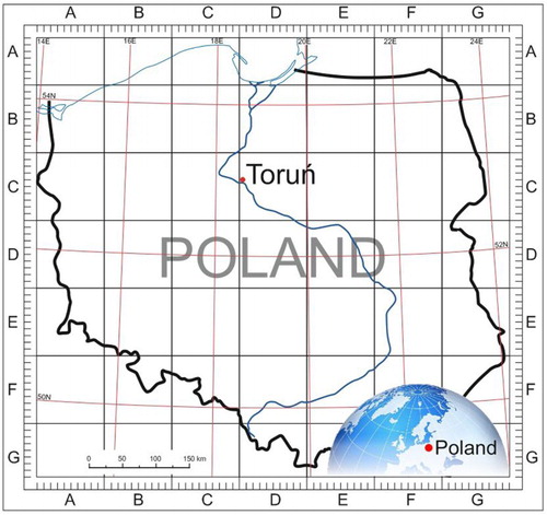
The analysed city is located in Central Poland in the Vistula valley on river terraces and dunes. Toruń is situated latitudinally on both sides of the river between the geographic latitudes of 52°58′ and 52°04′ and geographic longitudes of 18°32′ and 18°43′. The city covers approximately 115 km². In the ATPOL grid of squares, which uses the Cartesian coordinate system, Toruń occupies a field on the border between zones CC and DC. The cells are based on the Polish coordinate system according to Komsta (2016). The map of Toruń city covers a smallish region, so the curvature of the earth does not impact too much on the regular grids (Figure 1).

Figure 1. Location of the study area on a geographical grid and the ATPOL grid.

In recent years, since 2001 (the end of production by the large-scale chemicals firm Polchem), a significant improvement in air quality has been observed with regard to sulphur dioxide content. Unfortunately, a high level of atmospheric particulate matter persists (cf. Adamska, 2014).

The area where Toruń is situated is in a moderately warm climatic zone, and transitional between the oceanic climate of Western Europe to the continental climate of Eastern Europe and Asia (Wójcik & Marciniak, 1996).

Besides its climatic conditions being associated with its geographic location, the climate of Toruń exhibits the typical variations of urban areas and is not without the influence of biotic factors, including biota of lichen (cf. Adamska, 2014; Munzi et al., 2014). The spatial development of the city, its history, and the participation of green areas all influence the accessibility of habitats and substrates to lichens (cf. Adamska, 2014).

2. Methods

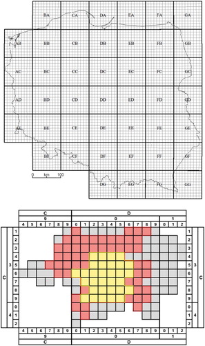
In implementing this semi-automated procedure, there is an initial subjective separating out of spatial features from source orthophotomaps, and then the high-resolution spatial data is divided into coarser grid cells. This provided a land-use map of the research area. After the subjective analysis, the data were calculated and processed using computer software. A synthetic map was created on the distribution of anthropogenic and natural factors, sulphur dioxide pollution and dominant natural environmental factors. The advantages of the procedure which was used come from the concept known as Operational Geographic Units (OGU) represented here by the ATPOL grid, which is a useful tool for the integration of multiple-source GIS data relating to a designated location on the Earth’s surface (Figure 2). This grid consists of basic square geometric fields of 10 × 10 km, which can be subdivided into fields of smaller area or grouped into squares of greater area. Polish geobotanists mainly use them for collating and presenting data on plant distributions (Komsta, 2016; Zając & Zając, 2001).

This automated method was used to determine the percentage share of particular elements of the geographic environment in individual fields. Automation was not used for classification. In many situations, a more-than-50% share was recorded for on dominant landscape element while, in a few cases, intervention with a researcher was needed for classification. Eleven such elements were analysed in order to determine the dominant-share environmental factor. Finally, these were aggregated to produce a total of six categories. The categories ‘Industrial area’, ‘Forest’, and ‘Water’ remained unchanged, on account of their high significance and surface share in the areas of the town. The aggregation did, however, affect: ‘road and compact settlement’, comprised of roads, compact settlement, unpaved roads; ‘urban greenery’, comprising fields, cemeteries, and airport; and ‘others’, which comprised other and railways. This meant that a 50% share was obtained for the dominant category in the cases being discussed.

Figure 2. Ten kilometres of geobotanic ATPOL grid, and 1-km grid of the city, divided into: yellow area – 1950s, red area – 1980s, black area – current town limits.

The standard in which the analysis was based was an orthophotomap, which was used to determine the land-use structure of the research area and its synthetic image of the city and the precise location of objects (Altobelli, Feoli, & Ourabia, 2001; Kot & Leśniak, 2017). With the support of a database on the urban area, elements of the city landscape were identified. The same database was used to identify areas with a predominance of industry, compact settlements and roads, forests and urban greenery (including squares, parks, and borders), water bodies and other miscellaneous anthropogenic areas. Ruderal areas were classified as ‘others’. The ATPOL grid was also marked up with the graded participation of anthropogenic factors, paying particular attention to SO₂ air pollution, and with the participation of natural factors. Formulae were created based on weightings for specific factors and their impact on the habitat requirements of the lichen species under analysis. The weightings of individual factors were determined subjectively by studying the influence of habitat factors on the occurrence of lichen, e.g. the impact of compact settlement and industrial area or forest area, etc. (Adamska, 2014). This reinforces the importance of individual factors and maintains the gradation between them. The aim was to characterise a cell in terms of habitat, with higher indices for a given factor denoting a greater impact on the potential for lichens to occur. A separate analysis of historical data was conducted (Main Map).

2.1. Anthropogenic factors

The participation of anthropogenic factors was determined by the degree of land development, which allowed individual study squares to be defined in this regard. The degree of land development for each square was calculated by:(1) where cs – compact settlement, ia – industrial area, r – roads, and rw – railways.

This yielded an image of the variability of anthropogenic factors, from least to most significant, in a four-tone colour scale.

2.2. Natural factors

As with the case of anthropogenic factors, natural factors were given an appropriate ranking. The degree of naturalness, i.e. the percentage participation of different environmental elements, was calculated by:(2) where fo – forest, fi – fields, o – other, w – waters, ur – unpaved roads, c – cemeteries, and a – airport.

The highest ranking was ascribed to wooded areas. ‘Other’ areas included greenfield areas, small anthropogenic woods, sandy grasslands, etc. Based on the data gained from this process, a four-tone colour scale was created, as with the anthropogenic factors.

2.3. SO₂ air pollution

The degree of SO₂ air pollution is presented as an isolated anthropogenic factor. It must be emphasised that because of the lack of air pollution measurements in Toruń, particularly for the 1950s and 1980s, sparsely available data on airborne sulphur dioxide concentrations for the town were used from a few measurement stations, which are both temporally and spatially irregular. In order to plot maps of environmental SO₂ contamination (μg/m³ of air), measurement results were averaged, with the data source being the databases of regional environmental protection inspectorates. Air pollution was calculated for the years 1950, 1980, and 2006, by:(3)

2.4. The dominant-share environmental factor

The dominant environmental element (by percentage share) is a synthesis of environmental elements which comprise the main share. The choropleth map is a visualisation of the factors which represent the largest percentage share of individual study fields and includes all dominant land uses in a square’s area, expressed by the equation:(4) where fo – forest, fi – fields, o – other, w – waters, ur – unpaved roads, c – cemeteries, a – airport, cs – compact settlement, ia – industrial area, r – roads, and rw – railways.

Here, squares dominated by industrial areas, roads, forests, fields, waters, and other greenfield areas are indicated. The participation of roads here is strictly associated with compact settlements. The image which was produced shows which environmental factors significantly influence the character of a square (or locality). Individual dominant land-use elements are presented with a colour scale.

The completed image is of the 144 ATPOL squares with a defined dominant share of individual elements which represent the features of the analysed lichens’ habitats. After drawing up the orthophotomaps (subjective interpretation and manual vectorisation), the obtained data were categorised and verified by field studies. The data thus obtained on percentage cover of particular urban landscape features were automatically analysed using JosekPLAN software (which collates pixels of the same colour on the ATPOL grid into fields and assigns each field a category according to its percentage-wise dominant feature). The resultant image shows dominant landscape features. Individual stages are presented in Figure 3.

Figure 3. Stages in the preparation of choropleth maps of the dominant-share of individual elements. (A) Orthophotomap (the resolution of input materials was 1.0 m), (B) land-use map of city, (C) dominant-share elements.

2.5. Histogram of frequency

The histogram of frequency on substrates shows the preferences of a given species to colonise a given substrate and is expressed as a percentage. It should be highlighted that, the data presented here is the author’s material from Adamska (2014) only. The histogram shows two values related to the substrate preferences of individual taxa, in the form of two differently coloured bars:

• average coverage on a given substrate across the whole study area, as a measure of abundance (shown as a red bar)

• percentage share of fields (squares) with the occurrence of a given substrate type, as a measure of frequency (shown as a green bar).

The histogram presented lists the Latin names of tree varieties in alphabetical order. The abbreviation ‘arb.al.’ is used to describe any type of phorophyte other than those listed in the histogram, such as: Juglan ssp., Larix sp., Malus sp., Padus sp., and Prunus sp. The substrate for epigeic lichens is described as ‘terra’, for quartzite substrates as ‘rupes’, and for artificial limestone substrates as ‘rupes_a’. Substrates for epixylic lichens are described as ‘lignum’. Other lichen substrates such as: other lichen, moss, anthropogenic substrates (old leather, slag, etc.) are expressed as ‘varia’.

2.6. Occurrence in historical study periods

Apart from the distribution of a given species of lichen (Adamska, 2014), the occurrence of that taxon is presented for the historical study periods (Wilkoń-Michalska, Glazik, & Kalińska, 1988).

In this case, in the face of a lack of data on abundance, according to Wilkoń-Michalska et al. (1988), the simple fact of an occurrence was marked in the appropriate ATPOL square, based on the data available in the literature. Such a visualisation makes it possible to analyse changes in the distribution of individual taxa, both in time and space. The area of lichenological studies from which the historical data are taken differs significantly from the contemporary area. In the 1950s, it was confined to the city centre, and was then significantly expanded.

2.7. Frequency

Frequency, i.e. information relating to the occurrence of the taxon in question, both contemporary and on the basis of historical data, is given as ‘n’ (number). This relates to the number of stations (squares) in which the presence of a given taxon of lichen was recorded in the three research periods, where:

• n – research from the years 2000–2006 (Adamska, 2014),

• n₈₀ – data from the 1980s (1974–1988), according to Wilkoń-Michalska et al. (1988),

• n₅₀ – data from the 1950s (up to 1952), according to Wilkoń-Michalska et al. (1988).

2.8. Occurrence and classification of lichens

The occurrence and classification of lichens according to Adamska (2014) is portrayed as appropriately sized circles. In this manner, both the fact of occurrence and the abundance of occurrence (i.e. the percentage of coverage on all available substrates) is portrayed in a given ATPOL study square. The authors believe that the proportional circles method is more legible than introducing new colours into the cartogram, hence the selection of this visualisation method.

2.9. Study material

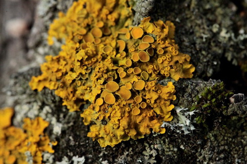
The study material was two species of lichen, Hypogymnia physodes (Figure 4) and Xanthoria parietina (Figure 5).

Figure 4. Hypogymnia physodes (phot. E. Adamska).

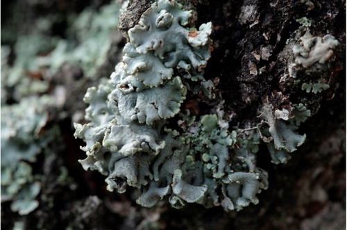
Figure 5. Xanthoria parietina (phot. E. Adamska).

The study covered all possible habitats and substrates for both species. Lichenological data were gathered from 137 squares. Samples were taken from all available substrates, both natural and anthropogenic, in a given square. Barks of the following species of trees and bushes were analysed for presence of lichens: Acer negundo, A. platanoides, Aesculus hippocastanum, Betula pendula, Populus alba, P. nigra, P. tremula, Pinus sylvestris, Quercusrobur, Q. rubra, Q. petraea, Salix alba, S. fragilis, Tilia mordata, T. platyphyllos and others.

In the case of epiphytic lichens, apart from their taxonomical classification and extent of coverage, the distribution on the analysed phorophyte was also studied from the foot of the trunk to a height of 2 m. Lichens also occurred on substrates of wood, such as fencing, wooden structures, logs and rail sleepers. Stone substrates were also penetrated, both anthropogenic limestones, such as concrete structures, electricity pylons, Eternit, walls (including historical structures), and non-limestones (silicates) such as stones, rocks, and stone pillars. For each listed species and each herbarium specimen taken for laboratory analysis, the type of colonised substrate and abundance of the taxon on a given substrate were described.

3. Conclusions

Data collected in the computer database has been represented using a choropleth map and diagrams. The base layer is the choropleth map, a grid of regular fields (equilateral quadrangles) – a quantitative method for representing cartographic phenomena which involves giving each spatial unit a colour fill dependent on the intensity of the phenomenon in question. In the case in question, it depicts: groups of factors (extent of land development, degree of naturalness, degree of air pollution) and elements (dominant land-use of a square, study period). Each diagram relates to only a single lichen species. Six classes were created, for each of which one type of diagram was produced, with fixed dimensions. The point size of a diagram depends on the percentage cover of the lichens in a given ATPOL square.

H. physodes most frequently and most abundantly occurred on the physiologically acidic bark of B. pendula and Pinus silvestris. Meanwhile, X. parietina, grew most frequently on Populus sp. and Acer sp. and on substrates containing calcium carbonate – concrete and mortar. X. parietina, being a nitrophilous and coniophilous species occurs mainly in anthropogenic locations – along transport routes and in built-up areas. The second of the species, the acidophilous H. physodes, prefers forest habitats, where it occurs most often and with greatest coverage. Both species are currently classed as common and occur in more than 70% of localities (squares). These species colonise various types of substrate.

Comparing to the historical data on the species in question, X. parietina significantly increased its number of stations from 28 in the 1950s and 1980s (Wilkoń-Michalska et al., 1988) to 99 stations in the years 2000–2006 (Adamska, 2014). Similarly, H. physodes expanded from 29–31 historical stations (1950s, 1988s) to its current 104 (2000–2006).

This graphic method allows the habitat preferences of the analysed taxa to be quickly evaluated through time and geographically. It is therefore possible to draw conclusions on the influence of urban conditions, such as changes in type and intensity of air pollutions (including, for example, sulphur oxides or particulate matter) on the species composition and distribution of lichens in the study area.

Software

The maps were produced using ArcGIS software. The authors’ proprietary software JosekPLAN was used for analysing aerial photographs and calculating individual elements of the city landscape. The authors’ proprietary software LichenSTAT was used for gathering lichen data (Adamska, 2014).

Acknowledgements

The authors would like to thank Reviewers for constructive comments and suggestions.

Disclosure statement

No potential conflict of interest was reported by the authors.

ORCID

Edyta Adamska http://orcid.org/0000-0001-5215-0666

Włodzimierz Juśkiewicz http://orcid.org/0000-0002-6755-3975

Additional information

Funding

This work was supported by Faculty of Biology and Environmental Protection, Nicolaus Copernicus University in Toruń.

References

- Adamska, E. (2014). Biota porostów Torunia na tle warunków siedliskowych miasta [Lichen biota in Toruń in relation to habitat conditions of the city] (pp. 1–212). Toruń: Wydawnictwo Naukowe Uniwersytetu Mikołaja Kopernika.
- Altobelli, A., Feoli, E., & Ourabia, L. (2001). An overview of landscape structure through the application of dimension to remotely sensed images using GIS technology. In A. Nienartowicz, & M. Kunz (Eds.), GIS and remote sensing in studies of landscape structure and function (pp. 39–50). Toruń: UMK.
- Bertin, J. (1981). Graphics and graphic information processing. Berlin: Walter de Gruyter and Company.
- Cleveland, W. S. (1993). Visualizing data. Summit, NJ: Hobart Press.
- Conti, M. E., & Cecchetti, G. (2001). Biological monitoring: Lichens as bioindicators of air pollution assessment – a review. Environmental Pollution, 114, 471–492. doi: 10.1016/S0269-7491(00)00224-4
- Davies, L., Bates, J. W., Bell, J. N. B., James, P. W., & Purvis, W. O. (2007). Diversity and sensitivity of epiphytes to oxides of nitrogen in London. Environmental Pollution, 146(2), 299–310. doi: 10.1016/j.envpol.2006.03.023
- Estrabou, C., Filippini, E., Soria, J. P., Schelotto, G., & Rodriguez, J. M. (2011). Air quality monitoring system using lichens as bioindicators in Central Argentina. Environmental Monitoring and Assessment, 182, 375–383. doi: 10.1007/s10661-011-1882-4
- Friendly, M. (2008). The golden age of statistical graphics. Statistical Science, 23(4), 502–535. doi: 10.1214/08-STS268
- Haberlie, A. M., Ashley, W., & Pingel, T. (2015). The effect of urbanisation on the climatology of thunderstorm initiation. Quarterly Journal of the Royal Meteorological Society, 141(688), 663–675. doi: 10.1002/qj.2499
- Komsta, Ł. (2016). Rewizja matematyczna siatki geobotanicznej ATPOL – propozycja algorytmów konwersji współrzędnych. Annales Universitatis Mariae Curie-Skłodowska, Sec. E, 71(1), 31–37.
- Kot, R., & Leśniak, K. (2017). Impact of different roughness coefficients applied to relief diversity evaluation: Chełmno Lakeland (Polish Lowland). Geografiska Annaler: Series A, Physical Geography, 99(2), 102–114. doi:10.1080/04353676.2017.1286547
- Lodha, A. S. (2013). Evaluation of various lichen species for monitoring pollution. Current Botany, 4(3), 63–66. ISSN: 2220-4822.
- MacEachren, A. M., & Taylor, D. R. F. (1994). Visualization in modern cartography: Setting the agenda. In A. M. MacEachren, & D. R. F. Taylor (Eds.), Visualization in modern cartography (pp. 1–12). Oxford: Pergamon.
- Munzi, S., Correia, O., Silva, P., Lopes, N., Freitas, C., Branquinho, C., Pinho, P., & Firn, J. (2014). Lichens as ecological indicators in urban areas: Beyond the effects of pollutants. Journal of Applied Ecology, 51(6), 1750–1757. doi: 10.1111/1365-2664.12304
- NashIII, T. H. (2009). Introduction. In T. H. NashIII (Ed.), Lichen biology (pp. 1–8). Cambridge: University Press.
- O’Brien, O., & Cheshire, J. (2016). Interactive mapping for large, open demographic data sets using familiar geographical features. Journal of Maps, 12(4), 676–683. doi: 10.1080/17445647.2015.1060183
- Robbins, N. B. (2005). Creating more effective graphs. Hoboken, NJ: John Wiley & Sons.
- Robinson, A. H., Morrison, J. L., Muehrcke, P. C., Kimerling, A. J., & Guptill, S. C. (1995). Elements of cartography (6th ed.). New York, NY: John Wiley & Sons.
- Slingsby, A., & van Loon, E. (2016). Exploratory visual analysis for animal movement ecology. Computer Graphics Forum, 35(3), 471–480. doi: 10.1111/cgf.12923
- Ulshöfer, J., & Rosner, H. J. (2001). GIS-based analysis of lichen mappings and air pollution in the area of Reutlingen (baden-wurttemberg, Germany). Meteorologische Zeitschrift, 10(4), 261–265. doi: 10.1127/0941-2948/2001/0010-0261
- Wilkoń-Michalska, J., Glazik, N., & Kalińska, A. (1988). Porosty miasta Torunia. Acta Univ. Nicolai Copernici. Biologia, 29(63), 210–253.
- Wójcik, G., & Marciniak, K. (1996). Klimat. In G. Wójcik, & K. Marciniak (Eds.), Zintegrowany Monitoring Środowiska Przyrodniczego – Stacja Bazowa w Koniczynce (pp. 56–76). Kraków: Państwowa Inspekcja Ochrony Środowiska. Uniwersytet Mikołaja Kopernika w Toruniu. Biblioteka Monitoringu Środowiska, Warszawa–Toruń.
- Zając, A., & Zając, M. (2001). Atlas rozmieszczenia roślin naczyniowych w Polsce (pp. 11–12). Kraków: Pracownia Chorologii Komputerowej Instytutu Botaniki Uniwersytetu Jagiellońskiego.