Average annual and seasonal Land Surface Temperature, Spanish Peninsular

ABSTRACT

The first long-term Land Surface Temperature (LST) maps for the Peninsular Spain at annual and seasonal time scales for 1981–2015 is presented in this work. A robust protocol for correcting and calibrating NOAA-AVHRR images and computing LST datasets at the spatial resolution of 1.1 km has been used. Simultaneously, maximum air temperature (Tmax) maps at the same spatial resolution have been produced using data from meteorological stations. The comparison between the two datasets resulted in statistically significant spatial correlations at annual and seasonal scales. Finally, the Normalized Difference Vegetation Index (NDVI) data were also compared with the obtained LST datasets and the results showed significant negative correlations between the two variables, especially in summer.

KEYWORDS:

• Land Surface Temperature
• NOAA-AVHRR
• maximum air temperature
• regression-based interpolation

1. Introduction

Climate change processes are demanding high spatial and temporal observational datasets for the evaluation of climate models and the interaction of the climate with natural elements (Hofstra, Haylock, New, Jones, & Frei, 2008). Although, minimum and maximum air temperature and total precipitation are the most commonly used gridded climate variables, there are still other key climate parameters to be derived from either ground-based stations or satellite observations. Among these parameters, Land Surface Temperature (LST) is an essential environmental variable, which is a direct driving force of turbulent heat fluxes and long-wave radiation exchanges (Maurer, Wood, Adam, Lettenmaier, & Nijssen, 2002; Nishida, Nemani, Running, & Glassy, 2003). LST is a key variable in formulating energy and water budgets at local through global scales (Anderson et al., 2008; Karnieli et al., 2010; Kustas & Anderson, 2009; Li et al., 2013; Zhang et al., 2008), and it has been widely used during the last decades in a variety of environmental processes including vegetation dynamic (Kogan, 2001), drought (Karnieli et al., 2010; Rabin, Temimi, Stepinski, & Bothwell, 2014), forest fires (Vlassova, Pérez-Cabello, Mimbrero, Llovería, & García-Martín, 2014), urban expansion (Meng & Dou, 2016; Voogt & Oke, 2003) and climate change (Hansen, Ruedy, Sato, & Lo, 2010; Kalma, McVicar, & McCabe, 2008; Weng, 2009; Zhang et al., 2008).

LST can be obtained by large wide infrared radiometric information from different sensors on board of satellite platforms, some of them recording this data from the early of the 1980s, being the LST from the National Oceanic and Atmospheric Administration Advanced Very High Resolution Radiometer data (NOAA-AVHRR hereafter) the most widely used to obtain long-term time series of the sea surface temperature (SST, e.g. Reynolds, Rayner, Smith, Stokes, & Wang, 2002). In continental areas, there are larger problems to retrieve LST given the diversity of land cover types with different emissivity (Becker & Li, 1990; Qin, Dall, Karni, & Berliner, 2001; Sobrino, Raissouni, & Li, 2001), land cover changes (Jin & Liang, 2006), etc.

In Spain, the majority of studies that analyzed surface parameters, estimated from remote sensing data, have focused on visible and near-infrared images to retrieve indices of vegetation activity (e.g. Del Barrio, Puigdefabregas, Sanjuan, Stellmes, & Ruiz, 2010; Hill, Stellmes, Udelhoven, Röder, & Sommer, 2008). Although several studies have focused on the development of algorithms for an accurate estimation of the LST from NOAA-AVHRR data (e.g. Coll, Caselles, Sobrino, & Valor, 1994; Sobrino, Coll, & Caselles, 1991), or used LST to improve air temperature mapping (Vogt, Viau, & Paquet, 1997), there is not still a study that explores the potential of the NOAA-AVHRR thermal infrared data to obtain long-term LST climatology at high spatial resolution over the past three decades.

The objective of this study is to use 34 years (July 1981–June 2015) of NOAA-AVHRR to (i) develop the first long-term LST dataset for the Peninsular Spain and (ii) infer robust annual and seasonal long-term LST climatology at a high spatial resolution (i.e. 1.1 km) never showed before for the region.

2. Materials and methods

2.1. Protocol for processing development of a historical NOAA-AVHRR LST dataset

AVHRR sensor collects information in two long-wave thermal infrared bands at 10.3–11.3 μm and 11.5–12.5 μm. The two thermal bands on board of the NOAA-AVHRR satellites show a spatial resolution of 1.1 km at the nadir, collected at images of around 2700 km wide. In the thermal infrared region, there is a direct emission of energy, which is directly related to the temperature of the surface (Becker & Li, 1990; Sobrino et al., 1991). According to the Planck thermodynamic law, the temperature of a body may be estimated according to its radiation, by means of the simple inversion of the Planck equation (e.g. Becker & Li, 1990; Snyder, Wan, Zhang, & Feng, 1998; Urban, Eberle, Hüttich, Schmullius, & Herold, 2013).

Here, we have used the historical daily NOAA-AVHRR dataset comprising 12,418 afternoon images from July 1981 to June 2015 for the entire Peninsular Spain. All the available daily images from 1981 to 1986 were acquired to the Dundee Satellite Reception Center. Images from 1986 to 1997 were required to the European Spatial Agency and rescued from the original tapes. Finally, the images from 1997 were obtained from the Advanced High Resolution Picture Transmission (AHRPT/HRPT) antennae located at the Centro de Recepción, Proceso, Archivo y Distribución de Imágenes de Observación de la Tierra (CREPAD) that the Spanish National Institute of Aerospace Technology (INTA) has in its Canaries Space Centre (Maspalomas, Gran Canaria). Software was designed and implemented in the IDL language to read the different NOAA-AVHRR satellites and convert all images to the same format. We used the complete range of available AVHRR bands (1–5) since in addition to the two thermal bands (4 and 5) used to calculate the LST, we needed the information from the visible, near-infrared and medium infrared spectral regions with the purpose of calculating the surface emissivity and obtaining robust cloud coverage masks.

The first step was to apply a geometric correction to the digital numbers (DN) of the NOAA-AVHRR images. For this purpose, we used the algorithm developed by Baena-Calatrava (2002), which is based first on the satellite parameters and second on geometric corrections. The second geometric correction uses a set of 97 Ground Control Points, which are based on recognizing land patterns (Ho & Asem, 1986) and are mostly located in coastal accident (e.g. capes), but also in land areas (e.g. reservoirs). The images were then re-projected to the European-ED50-UTM zone 30N over an area bounded between 34°22′N and 44°12′N and 11°7′W and 4°16′E.

The second step was to calibrate the different satellites (Price, 1991). Initially, we applied a linear correction to obtain the radiance recorded by the satellite (L_a) from the DNs, using the coefficients embedded in the images (G and I), for bands 4 and 5. These coefficients are different for each line of the image.$L_a=\text{G}\times \text{DN}+\text{I}$The radiances were corrected non-linearly for the satellites N-7, N-9, N-11 and N-14:$L=A{L}_a+B{L}_a^2+C$where A, B and C are coefficients that can be retrieved from Walton, Sullivan, Rao, and Weinreb (1998) for NOAA-7 to NOAA-14 satellites and in the NOAA user guide for NOAA-16, NOAA-18 and NOAA-19 (http://www.ncdc.noaa.gov/oa/pod-guide/ncdc/docs/klm/html/d/app-d2.htm; last accessed 1 February 2017).

Brightness temperatures (T_B) were obtained from radiances according to the Planck equation:$T_B=\frac{c_{2}v}{ln\left(1+{\displaystyle \frac{c_1{v}^3}{L}}\right)}$where c₁ = 1.1910659 × 10⁻⁵ m W sr⁻¹ cm⁴, c₂ = 1.438833 cm K. The values of v change for each satellite and they can be found in the NOAA satellite specifications (http://www.ncdc.noaa.gov/oa/pod-guide/ncdc/docs/podug/html/c1/sec1-4.htm; last accessed 1 February 2017).

Once brightness temperatures were obtained, we removed cloudy pixels. For this purpose, we used the cloud detection algorithm developed by Azorin-Molina et al. (2013) also implemented in the IDL software. To avoid problems related to cloud shadows, we also removed three pixels around the identified cloudy pixels. In addition, to avoid geometric and radiometric problems related to the view angle of satellites, we removed those pixels with observation angles higher than 50°.

Red and near-infrared bands were calibrated using revised calibration coefficients considering the orbit degradation for each satellite (Rao & Chen, 1995, 1999; http://www.ncdc.noaa.gov/oa/pod-guide/ncdc/docs/intro.htm; last accessed 1 February 2017). Channel 1 and 2 radiances were transformed to top-of-the-atmosphere reflectances and cross-calibrated to the NOAA-9 sensor to correct the different spectral response of the sensors (Trishchenko, 2009; Trishchenko, Cihlar, & Li, 2002), and finally the reflectances were topographically corrected by means of a non-Lambertian model using a digital elevation model at the resolution of 1.1 km (Riaño, Chuvieco, Salas, & Aguado, 2003).

To obtain the LST, we applied a split-window algorithm developed by Sobrino and Raissouni (2000) and widely tested by the atmospheric conditions of the Iberian Peninsula:$\text{LST}=T_4+c_1(T_4-T_5)+c_2(T_4+T_5{)}^2+c_0+(c_3+c_{4}W\left)\right(1-\epsilon )+(c_5+c_{6}W)\mathrm{\Delta }\epsilon$where W is the water vapor content in each pixel of the image, according to the algorithm by Sobrino, Jimenez, Raissouni, and Soria (2002), valid for the latitudes in which the Iberian Peninsula is located:$W=0.259-14.253(\cos \theta \text{ln}R)-11.649(\cos \theta \text{ln}R{)}^2$

R is obtained for the whole pixels available in the image (free of clouds and lower than 50° of view angle).$R=\frac{{\sum }_{K=1}^N(T_{4,k}-T_{4,0})(T_{5,k}-T_{5,0})}{{\sum }_{K=1}^N{(T_{4,k}-T_{4,0})}^2}$

T_4,k is the value of the pixel k in the band 4; T_4,0 is the average of all the available pixels in the band 4; T_5,k is the value of the pixel k in the band 5; T_5,0 is the average of all the pixels in the band 5. The emissivity ε and Δε are obtained according to the method developed by Sobrino et al. (2008) using thresholds of the Normalized Difference Vegetation Index (NDVI) values from the red and near-infrared bands. The coefficients c₀ to c₆ were obtained from Lahraoua, Raissouni, Chahboun, Azyat, and Achhab (2012). For inland water bodies and given they are relatively small in Spain, we did not apply a different algorithm for them. We considered that the same algorithm used to estimate the LST is valid for water areas changing the value of emissivity corresponding to the water. This was addressed in the emissivity methodology (Sobrino et al., 2008) used in this study.

LST may vary as a function of the viewing angle (Wan & Dozier, 1996), but also as a function of the time at which the images are taken, given the different sun angles and radiation received by the surface (Price, 1991). Julien and Sobrino (2012) illustrated this problem and demonstrated that orbit drift is an important source of noise in LST time series. The difficulties of developing a physical approach to correct these effects motivated the use of a statistical approach, similar to that followed by Julien and Sobrino (2012) to remove from each daily LST image the effects of the different solar zenith and observation angles. Given the strong seasonality found in solar effects, we split the available daily time series in semimonthly series (all the images between 1st January and 15th January, between 16th January and 31st January and so on). This selection produced 24 series of LST for the period 1981–2015. For each series and pixel, we removed the effect of the zenith and observation angles by means of a multiple regression model:$\text{LST}=a+b\ast a_z+c\ast a_o$where a, b and c are the regression coefficients and a_z and a₀ are the solar zenith and observation angles, respectively. Using the coefficients obtained, we calculated the free-effect LST (LST_c) removing the obtained residuals (observed minus predicted LST by the model) according to:$\text{LST\_c}=m+(\text{LST}-(a+az\ast b+ao\ast c\left)\right)$where m is the average LST in the semimonthly time series.

Daily images were composited in semimonthly periods (two per month, from the 1st day of the month to the 15th, and from 16th to the end of the month) using the maximum temperature recorded in the period. The use of maximum LST values instead of the mean of the semimonthly periods was made to ensure the minimum effect of any remaining cloud coverage on our data. Moreover, as a function of the dates in which data is available the mean values may produce strong spatial contrasts mostly driven by data availability. On the other hand, and as recommended by NDVI, maximum instead mean values also produce much better results in terms of spatial and temporal homogeneity of the resulting LST.

The large number of images affected by clouds, large observation angles and geometric distortions caused several gaps in the data series. To fill these gaps we used a regression model considering the LST values of the series of the pre- and post-semimonthly periods as predictors. The procedure was applied iteratively to complete all the gaps existing in the images and to make sure all consecutive periods with no data are correctly filled. The series of each pixel were temporally filtered to reduce residual noise by means of the algorithm developed by Quarmby, Milnes, Hindle, and Silleos (1993), which filters low LST values since high LST values are less affected by atmospheric contamination and residual noise.$\text{LST}=\text{Max}\{\text{LS}{\text{T}}_{\left(n\right)},(\text{LS}{\text{T}}_{(n-1)}+\text{LS}{\text{T}}_{(n+1)})/2\}$

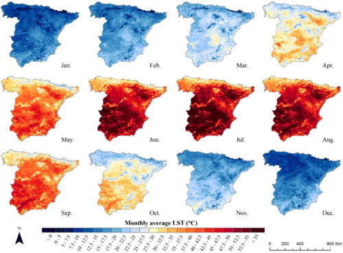
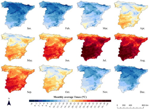
Finally, the semimonthly images were used to create monthly, seasonal (defined as winter (DJF), spring (MAM), summer (JJA), autumn (SON)) and annual series, using the average values for each period. Figure 1 shows a summarizing schema of the main steps of the LST dataset development and Figure 2 shows an example of the monthly images from January to December 2010 as an example.

Figure 1. Diagram of the protocol adopted to derive LST data from NOAA-AVHRR images between 1981 and 2015.

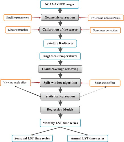
Figure 2. Spatial variability of the average monthly LST during 2010.

2.2. Spatial modeling of air temperature

2.2.1. Air temperature data

To deepen the knowledge of the relationship between the spatial variability of the LST retrieved from NOAA-AVHRR images and air temperature, we have used the available information on air temperature in Spain. There are different gridded layers of air temperature in Spain (e.g. Gonzalez-hidalgo, Peña-angulo, & Cortesi, 2015; Herrera, Fernández, & Gutiérrez, 2016). Nevertheless, these datasets show low spatial resolutions to be compared with the high spatial resolution (1.1 km) of the LST dataset created in this study. For this reason, we have developed a new monthly gridded dataset for the period 1981–2015 to match with the spatial resolution of the LST images. We have focused on maximum air temperatures (Tmax) since they are more comparable to the LST.

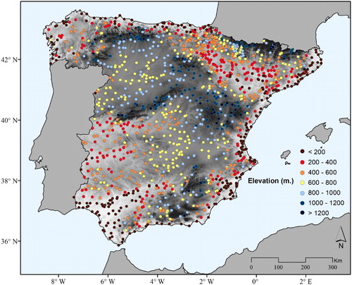
To generate a gridded dataset for air temperature, we have used the most complete, quality controlled and homogenized dataset available for Spain, based on the Monthly Temperature Data for Spain (MOTEDAS) dataset (Gonzalez-hidalgo et al., 2015). This dataset contains more than 1300 stations over Spain. The dataset was updated to 2015 using the raw time series of air temperature from the Spanish National Meteorological Agency (AEMET), and the few existing gaps filled by means of the use of reference series, following the same approach used by Gonzalez-hidalgo et al. (2015) to generate the MOTEDAS dataset. A total number of 1348 meteorological stations, which cover the entire study domain, were used to generate the gridded layers (Figure 3).

Figure 3. Network of meteorological stations by altitudinal intervals.

2.2.2. Regression-based approach

To generate the gridded layers at the spatial resolution of 1.1 km, we applied a regression-based approach (Ninyerola, Pons, & Roure, 2000). For this purpose, we used different geographic and topographic variables that affect the spatial distribution of air temperatures (i.e. elevation, distance to the sea, latitude and longitude) that were incorporated as independent layers in the generation of global regression models in which the dependent variable was Tmax. Correlation between variables (collinearity) can complicate the interpolation of the results. To prevent this problem, a forward stepwise procedure, with ‘probability to enter’ set to .05, was used to select only significant variables (Hair, Anderson, Tatham, & Black, 1998).

Air temperature predictions by the linear regression models are inexact since usually there is a difference between the observed and predicted air temperature values in the location of the points of observation. For this reason, we applied a local interpolation of the residual values (observed minus predicted) to obtain exact values in the points of measurement by means of the difference between the regression results and the interpolated residuals. For this purpose, a kriging algorithm was used considering independent spherical semivariograms for each month.

2.2.3. Validation of the predictions

To determine the quality of the Tmax predictions, the grid layers were validated by a Jackknife resampling procedure (Phillips, Dolph, & Marks, 1992). This approach is based on withholding, in turn, one station out of the network, estimating regression coefficients from the remaining observatories, locally interpolating the residuals and calculating the difference between the predicted and observed value for each withheld observatory. We calculated two validation statistics by means of the comparison between the observed and predicted values of each monthly layer: the mean absolute error (MAE) and the agreement index (D) (Willmott, 1981), which are relative and bounded measures of model validity.

Figure 4 shows the temporal evolution of D (blue) and MAE (red) in the different monthly gridded data created. These results indicate the good quality of predictions since D values are always higher than 0.9 and they are close to 0.95 most of the months, which indicates a high agreement between observations and predictions. The MAE oscillates around 1°C, being the errors a bit higher for winter than for summer months. Figure 5 presents an example of the obtained grids corresponding to the average monthly maps of Tmax over the Peninsular Spain during 2010 in which there is certain spatial and seasonal agreement of the maps to the obtained results for the LST during the same year.

Figure 4. Evolution of the Willmott’s D (blue) and the MAE (red) from the Jackknife validation approach.

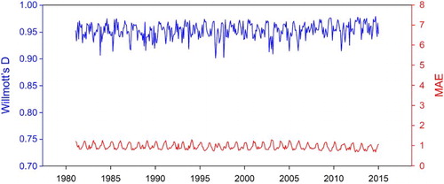
Figure 5. Spatial variability of the average monthly Tmax during 2010.

2.3. Normalized Difference Vegetation Index

To study the interaction between the spatial variability of the LST and the vegetation coverage, we have used the NDVI dataset at the same spatial resolution of 1.1 km. The NDVI dataset has recently been developed by Martin-Hernandez et al. (2017) using the same NOAA-AVHRR dataset processed in this study therefore covering the same spatial and temporal coverage.

3. Results

The Main Map shows the spatial distribution of the average annual and seasonal LST in the Peninsular Spain for 1981–2015 showing marked spatial and seasonal differences. Summer is the season that recorded the highest values, in some areas of the South and Southwest higher than 55°C. Also in areas of the Northeast, in the semiarid regions of the Ebro river basin, LST greater than 50°C have been recorded in summer. In spring and autumn, the spatial distribution of the LST is highly controlled by the relief disposition, with low LST recorded in the different topographic chains (the Pyrenees, Central system, etc.). In winter, dominated a North–South gradient, with the lowest temperatures recorded in the northern chains (the Pyrenees, Cantabrian mountains), and also in the northern plateau of the Iberian Peninsula. Annual distribution of LST shows a mixture of these seasonal patterns. There is a high topographic control, but also clear latitudinal gradient, which is modulated by the spatial distribution of the vegetation coverage.

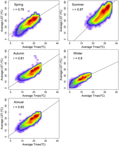
The observed spatial distribution of LST is strongly related to the spatial distribution of the average Tmax at seasonal and annual scales (Figures 6 and 7). The spatial distribution of the average annual Tmax also shows higher values in the southwestern and southeastern parts of Spain. The Guadalquivir valley shows the highest average values and the lowest values are recorded in the North, corresponding to the Pyrenees and the Cantabrian range. The maps show strong seasonality in the air temperature, but independently of the season of the year, the spatial patterns are very close to that observed for the average LST.

Figure 6. Spatial distribution of annual and seasonal average maximum air temperature.

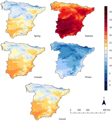
Figure 7. Relationship between the average LST and the maximum air temperature at seasonal and annual scales. The colors represent the density of points.

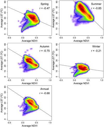
Nevertheless, there is also a close relationship with the spatial distribution of the vegetation activity, represented by the NDVI. The average LST shows a negative and strong correlation with the average NDVI (Figure 8), indicating that areas that show higher vegetation activity/coverage tend to show a lower LST than areas showing nude soils or low vegetation coverage. Thus, at the annual scale, the correlation is strong among these two variables (r = −0.68).

Figure 8. Relationship between the average LST and the NDVI at seasonal and annual scales. The colors represent the density of points.

4. Conclusion

This study develops a long-term database (1981–2015) of LST at a high spatial resolution (1.1 km²) from the set of NOAA-AVHRR images available in the Peninsular Spain, which were obtained after processing the thermal infrared bands (4 and 5) using a split-window algorithm. This dataset has improved the spatial resolution of previous available datasets for Spain, i.e. the Pathfinder 64 km² – (Julien, Sobrino, & Verhoef, 2006; Ouaidrari, Goward, Czajkowski, Sobrino, & Vermote, 2002) and the Land Long Term Data Record (LTDR) 16 km² (Sobrino & Julien, 2016).

The study analyzed for the first time the spatial patterns of the long-term high spatial resolution (1.1 km²) LST for the Peninsular Spain. The LST climatology shows more spatial details and contrasts than the available air surface temperature climatology for Spain (e.g. http://www.opengis.uab.es/wms/iberia/mms/index.htm) since it allows to identify features related to the terrain conditions (e.g. vegetation coverage and type) and to cover areas in which the availability of meteorological stations is low.

There are important spatial and seasonal differences of the LST across Spain. Nevertheless, strong agreement between the spatial distribution of the average LST and the average Tmax has been found. In addition, we have also showed that other factors may also contribute to explain the spatial distribution of the LST. The principal of these factors is the spatial distribution of the vegetation coverage, being mainly evident during the summer season, in which the contrasts between the areas covered by vegetation and areas of nude soil are clearer in terms of radiative fluxes (Kustas & Anderson, 2009). Thus, in the summer season, there is a negative and linear relationship between the spatial distribution of the LST and the NDVI, which is also identified at the annual scale. The strong relationship between the average distribution of the LST and the NDVI has implications to understand current soil moisture differences, which can be determined by means of conceptual models based on the combination between LST and NDVI (Sandholt, Rasmussen, & Andersen, 2002).

The gridded seasonal and annual climatology layers of LST and air temperature for continental Spain are available in Ascii ESRI format at the Institutional Repository of the Spanish National Research Council (http://hdl.handle.net/10261/164053).

Software

Interactive Data Language (IDL) software was developed to process the daily NOAA-AVHRR images. R 3.3.2 was used to develop the seasonal and annual dataset of LST. MiraMon 6.4 and Idrisi Taiga were used to model mean air temperature. ArcGis 10.2 was used to generate the final maps.

Disclosure statement

No potential conflict of interest was reported by the authors.

ORCID

Makki Khorchani http://orcid.org/0000-0001-9379-7052

Additional information

Funding

This work was supported by the research projects I-Link1001 (Validation of climate drought indices for multi-sectorial applications in North America and Europe under a global warming scenario) financed by Consejo Superior de Investigaciones Científicas [PCIN-2015-220, CGL2014-52135-C03-01], Red de variabilidad y cambioclimático RECLIM (CGL2014-517221-REDT) financed by the Spanish Foundation for Science and Technology and FEDER European Regional Development Fund, IMDROFLOOD financed by the Water Works 2014 Joint Programming Initiative Water challenges for a changing world co-funded call of the European Commission, and ‘LIFE12 ENV/ES/000536-Demonstration and validation of innovative methodology for regional climate change adaptation in the Mediterranean area (LIFE MEDACC)’ financed by the LIFE Financial Instrument for the Environment program of the European Commission.

References

- Anderson, M. C., Norman, J. M., Kustas, W. P., Houborg, R., Starks, P. J., & Agam, N. (2008). A thermal-based remote sensing technique for routine mapping of land-surface carbon, water and energy fluxes from field to regional scales. Remote Sensing of Environment, 112, 4227–4241. doi: 10.1016/j.rse.2008.07.009
- Azorin-Molina, C., Baena-Calatrava, R., Echave-Calvo, I., Connell, B. H., Vicente-Serrano, S. M., & López-Moreno, J. I. (2013). A daytime over land algorithm for computing AVHRR convective cloud climatologies for the Iberian Peninsula and the Balearic Islands. International Journal of Climatology, 33, 2113–2128. doi: 10.1002/joc.3572
- Baena-Calatrava, R. (2002). Georreferenciacion automatica de imagenes NOAA-AVHRR (Master thesis). University of Jaen, Spain.
- Becker, F., & Li, Z.-L. (1990). Towards a local split window method over land surfaces. International Journal of Remote Sensing, 11, 369–393. doi: 10.1080/01431169008955028
- Coll, C., Caselles, V., Sobrino, J. A., & Valor, E. (1994). On the atmospheric dependence of the split-window equation for land surface temperature. International Journal of Remote Sensing, 15, 105–122. doi: 10.1080/01431169408954054
- Del Barrio, G., Puigdefabregas, J., Sanjuan, M. E., Stellmes, M., & Ruiz, A. (2010). Assessment and monitoring of land condition in the Iberian Peninsula, 1989–2000. Remote Sensing of Environment, 114, 1817–1832. doi: 10.1016/j.rse.2010.03.009
- Gonzalez-hidalgo, J. C., Peña-angulo, D., & Cortesi, N. (2015). MOTEDAS: A new monthly temperature database for mainland Spain and the trend in temperature (1951–2010). International Journal of Climatology, 35, 4444–4463. doi: 10.1002/joc.4298
- Hair, J. F., Anderson, R. E., Tatham, R. L., & Black, W. C. (1998). Multivariate data analysis. New York, NY: Prentice Hall.
- Hansen, J., Ruedy, R., Sato, M., & Lo, K. (2010). Global surface temperature change. Reviews of Geophysics, 48, 644. doi:10.1029/2010RG000345.1.INTRODUCTION doi: 10.1029/2010RG000345
- Herrera, S., Fernández, J., & Gutiérrez, J. M. (2016). Update of the Spain02 gridded observational dataset for EURO-CORDEX evaluation: Assessing the effect of the interpolation methodology. International Journal of Climatology, 36, 900–908. doi: 10.1002/joc.4391
- Hill, J., Stellmes, M., Udelhoven, T., Röder, A., & Sommer, S. (2008). Mediterranean desertification and land degradation. Mapping related land use change syndromes based on satellite observations. Global and Planetary Change, 64, 146–157. doi: 10.1016/j.gloplacha.2008.10.005
- Ho, D., & Asem, A. (1986). NOAA AVHRR image referencing. International Journal of Remote Sensing, 7, 895–904. doi: 10.1080/01431168608948898
- Hofstra, N., Haylock, M., New, M., Jones, P., & Frei, C. (2008). Comparison of six methods for the interpolation of daily, European climate data. Journal of Geophysical Research, 113, D05109. doi: 10.1029/2008JD010100
- Jin, M., & Liang, S. (2006). An improved land surface emissivity parameter for land surface models using global remote sensing observations. Journal of Climate, 19, 2867–2881. doi: 10.1175/JCLI3720.1
- Julien, Y., & Sobrino, J. A. (2012). Correcting AVHRR Long Term Data Record V3 estimated LST from orbital drift effects. Remote Sensing of Environment, 123, 207–219. doi: 10.1016/j.rse.2012.03.016
- Julien, Y., Sobrino, J. A., & Verhoef, W. (2006). Changes in land surface temperatures and NDVI values over Europe between 1982 and 1999. Remote Sensing of Environment, 103, 43–55. doi: 10.1016/j.rse.2006.03.011
- Kalma, J. D., McVicar, T. R., & McCabe, M. F. (2008). Estimating land surface evaporation: A review of methods using remotely sensed surface temperature data. Surveys in Geophysics, 29, 421–469. doi: 10.1007/s10712-008-9037-z
- Karnieli, A., Agam, N., Pinker, R. T., Anderson, M., Imhoff, M. L., Gutman, G. G., … Goldberg, A. (2010). Use of NDVI and land surface temperature for drought assessment: Merits and limitations. Journal of Climate, 23, 618–633. doi: 10.1175/2009JCLI2900.1
- Kogan, F. N. (2001). Operational space technology for global vegetation assessment. Bulletin of the American Meteorological Society, 82, 1949–1964. doi:10.1175/1520-0477(2001)082<1949:OSTFGV>2.3.CO;2.
- Kustas, W., & Anderson, M. (2009). Advances in thermal infrared remote sensing for land surface modeling. Agricultural and Forest Meteorology, 149, 2071–2081. doi: 10.1016/j.agrformet.2009.05.016
- Lahraoua, M., Raissouni, N., Chahboun, A., Azyat, A., & Achhab, N. B. (2012). Split-window LST algorithms estimation from AVHRR/NOAA satellites (7, 9, 11, 12, 14, 15, 16, 17, 18, 19) using Gaussian filter function. International Journal of Information and Network Security (IJINS), 2, 68. doi: 10.11591/ijins.v2i1.1502
- Li, Z., Tang, B., Wu, H., Ren, H., Yan, G., Wan, Z., … Sobrino, J. A. (2013). Satellite-derived land surface temperature: Current status and perspectives. Remote Sensing of Environment, 131, 14–37. doi: 10.1016/j.rse.2012.12.008
- Martin-Hernandez, N., Vicente-Serrano, S. M., Azorín-Molina, C., Beguería, S., Reig, F., & Zabalza-Martínez, J. (2017, September 18–22). Three decades of NOAA-AVHRR data to assess vegetation dynamics in the Iberian Peninsula and the Balearic Islands. In J. A. Sobrino (Ed.). Proceedings of the 5th International Symposium on Recent Advances in Quantitative Remote Sensing RAQRS-V. Torrent, Spain: University of Valencia.
- Maurer, E. P., Wood, A. W., Adam, J. C., Lettenmaier, D. P., & Nijssen, B. (2002). A long-term hydrologically based dataset of land surface fluxes and states for the conterminous United States. Journal of Climate, 15, 3237–3251. doi: 10.1175/1520-0442(2002)015<3237:ALTHBD>2.0.CO;2
- Meng, C., & Dou, Y. (2016). Quantifying the anthropogenic footprint in eastern China. Scientific Reports, 6, 158. doi: 10.1038/srep24337
- Ninyerola, M., Pons, X., & Roure, J. M. (2000). A methodological approach of climatological modeling of air temperature and precipitation. International Journal of Climatology, 1841, 1823–1841.
- Nishida, K., Nemani, R. R., Running, S. W., & Glassy, J. M. (2003). An operational remote sensing algorithm of land surface evaporation. Journal of Geophysical Research: Atmospheres, 108, 4270. doi: 10.1029/2002JD002062
- Ouaidrari, H., Goward, S. N., Czajkowski, K. P., Sobrino, J. A., & Vermote, E. (2002). Land surface temperature estimation from AVHRR thermal infrared measurements: An assessment for the AVHRR Land Pathfinder II data set. Remote Sensing of Environment, 81, 114–128. doi: 10.1016/S0034-4257(01)00338-8
- Phillips, D. L., Dolph, J., & Marks, D. (1992). A comparison of geostatistical procedures for spatial analysis of precipitation in mountainous terrain. Agricultural and Forest Meteorology, 58, 119–141. doi: 10.1016/0168-1923(92)90114-J
- Price, J. C. (1991). Timing of NOAA afternoon passes. International Journal of Remote Sensing, 12, 193–198. doi: 10.1080/01431169108929644
- Qin, Z., Dall, G., Karni, A., & Berliner, P. (2001). Derivation of split window algorithm and its sensitivity analysis for retrieving land surface temperature from NOAA-advanced very high resolution radiometer data. Journal of Geophysical Research, 106670(16), 655–622. doi: 10.1029/2000JD900452
- Quarmby, N. A., Milnes, M., Hindle, T. L., & Silleos, N. (1993). The use of multi-temporal NDVI measurements from AVHRR data for crop yield estimation and prediction. International Journal of Remote Sensing, 14, 199–210. doi: 10.1080/01431169308904332
- Rabin, R. M., Temimi, M., Stepinski, J., & Bothwell, P. D. (2014). Monitoring surface dryness using geostationary thermal observations. Remote Sensing Letters, 5(1), 10–18. doi: 10.1080/2150704X.2013.862601
- Rao, C. R. N., & Chen, J. (1995). Inter-satellite calibration linkages for the visible and near-infrared channels of the advanced very high resolution radiometer on the NOAA-7, -9, and -11 spacecraft. International Journal of Remote Sensing, 16, 1931–1942. doi: 10.1080/01431169508954530
- Rao, C. R. N., & Chen, J. (1999). Revised post-launch calibration of the visible and near-infrared channels of the Advanced Very High Resolution Radiometer (AVHRR) on the NOAA-14 spacecraft. International Journal of Remote Sensing, 20, 3485–3491. doi: 10.1080/014311699211147
- Reynolds, R. W., Rayner, N. A., Smith, T. M., Stokes, D. C., & Wang, W. (2002). An improved in situ and satellite SST analysis for climate. Journal of Climate, 15, 1609–1625. doi:10.1175/1520-0442(2002)015<1609:AIISAS>2.0.CO;2
- Riaño, D., Chuvieco, E., Salas, J., & Aguado, I. (2003). Assessment of different topographic corrections in Landsat-TM data for mapping vegetation types. IEEE Transactions on Geoscience and Remote Sensing, 41, 1056–1061. doi: 10.1109/TGRS.2003.811693
- Sandholt, I., Rasmussen, K., & Andersen, J. (2002). A simple interpretation of the surface temperature/vegetation index space for assessment of surface moisture status. Remote Sensing of Environment, 79, 213–224. doi: 10.1016/S0034-4257(01)00274-7
- Snyder, W. C., Wan, Z., Zhang, Y., & Feng, Y. Z. (1998). Classification-based emissivity for land surface temperature measurement from space. International Journal of Remote Sensing, 19, 2753–2774. doi: 10.1080/014311698214497
- Sobrino, J. A., Jimenez, J. C., Raissouni, N., & Soria, G. (2002). A simplified method for estimating the total water vapor content over sea surfaces using NOAA-AVHRR channels 4 and 5. IEEE Transactions on Geoscience and Remote Sensing, 40, 357–361. doi: 10.1109/36.992796
- Sobrino, J. A., Jiménez-Muñoz, J. C., Sòria, G., Romaguera, M., Guanter, L., Moreno, J., … Martínez, P. (2008). Land surface emissivity retrieval from different VNIR and TIR sensors. IEEE Transactions on Geoscience and Remote Sensing, 46, 316–327. doi: 10.1109/TGRS.2007.904834
- Sobrino, J. A., & Julien, Y. (2016). Exploring the validity of the long-term data record V4 database for land surface monitoring. IEEE Journal of Selected Topics in Applied Earth Observations and Remote Sensing, 9, 3607–3614. doi: 10.1109/JSTARS.2016.2567642
- Sobrino, J. A., & Raissouni, N. (2000). Toward remote sensing methods for land cover dynamic monitoring: Application to Morocco. International Journal of Remote Sensing, 21, 353–366. doi: 10.1080/014311600210876
- Sobrino, J. A., Raissouni, N., & Li, Z.-L. (2001). A comparative study of land surface emissivity retrieval from NOAA data. Remote Sensing of Environment, 75, 256–266. doi: 10.1016/s0034-4257(00)00171-1
- Sobrino, J., Coll, C., & Caselles, V. (1991). Atmospheric correction for land surface temperature using NOAA-11 AVHRR channels 4 and 5. Remote Sensing of Environment, 38, 19–34. doi: 10.1016/0034-4257(91)90069-I
- Trishchenko, A. P. (2009). Effects of spectral response function on surface reflectance and NDVI measured with moderate resolution satellite sensors: Extension to AVHRR NOAA-17, 18 and METOP-A. Remote Sensing of Environment, 113, 335–341. doi: 10.1016/j.rse.2008.10.002
- Trishchenko, A. P., Cihlar, J., & Li, Z. (2002). Effects of spectral response function on surface reflectance and NDVI measured with moderate resolution satellite sensors. Remote Sensing of Environment, 81, 1–18. doi: 10.1016/S0034-4257(01)00328-5
- Urban, M., Eberle, J., Hüttich, C., Schmullius, C., & Herold, M. (2013). Comparison of satellite-derived land surface temperature and air temperature from meteorological stations on the Pan-Arctic scale. Remote Sensing, 5, 2348–2367. doi: 10.3390/rs5052348
- Vlassova, L., Pérez-Cabello, F., Mimbrero, M. R., Llovería, R. M., & García-Martín, A. (2014). Analysis of the relationship between land surface temperature and wildfire severity in a series of Landsat images. Remote Sensing, 6(7), 6136–6162. doi: 10.3390/rs6076136
- Vogt, J. V., Viau, A. A., & Paquet, F. (1997). Mapping regional air temperature fields using satellite-derived surface skin temperatures. International Journal of Climatology, 17(November), 1559–1579. doi:10.1002/(SICI)1097-0088(19971130)17:14<1559::AID-JOC211>3.0.CO;2-5
- Voogt, J. A., & Oke, T. R. (2003). Thermal remote sensing of urban climates. Remote Sensing of Environment, 86, 370–384. doi: 10.1016/S0034-4257(03)00079-8
- Walton, C. C., Sullivan, J. T., Rao, C. R. N., & Weinreb, M. P. (1998). Corrections for detector nonlinearities and calibration inconsistencies of the infrared channels of the advanced very high resolution radiometer. Journal of Geophysical Research: Oceans, 103, 3323–3337. doi: 10.1029/97JC02018
- Wan, Z., & Dozier, J. (1996). A generalized split-window algorithm for retrieving land-surface temperature from space. IEEE Transactions on Geoscience and Remote Sensing, 34, 892–905. doi: 10.1109/36.508406
- Weng, Q. (2009). Thermal infrared remote sensing for urban climate and environmental studies: Methods, applications, and trends. ISPRS Journal of Photogrammetry and Remote Sensing, 64, 335–344. doi: 10.1016/j.isprsjprs.2009.03.007
- Willmott, C. J. (1981). On the validation of models. Physical Geography, 2, 184–194. doi: 10.1080/02723646.1981.10642213
- Zhang, R., Tian, J., Su, H., Sun, X., Chen, S., & Xia, J. (2008). Two improvements of an operational two-layer model for terrestrial surface heat flux retrieval. Sensors, 8, 6165–6187. doi: 10.3390/s8106165