Flood hazard of major river segments, Benevento Province, Southern Italy

ABSTRACT

On 15 October 2015, a storm-induced flood hit the central sector of Benevento Province (southern Italy) causing two deaths and severe damage to infrastructure, buildings and local agriculture. This area has a long history of similar events and since 1924 its major river segments have been monitored with several hydrometric stations. We used data from two of these stations and a LiDAR derived high-resolution topography to develop a flood hazard map. For map computation, we first derived a flood inundation map from topography. Subsequently we estimated the probability of exceedance of each specific fluvial stage from the combination of a Generalized Extreme Value and a Gamma fits of available hydrometric data. As boundary condition, we considered a reference scenario corresponding to an estimated 500 year flood. The hazard maps provide an overview of the flood hazard in the central sector of Benevento Province and floodplains zonation in flood perspective.

KEYWORDS:

• Flood
• hazard
• LiDAR
• Sentinel 2
• probability analysis
• return period

1. Introduction

In the last three decades, ongoing climate change has been responsible for a global increase in the frequency and magnitude of heavy precipitation (e.g. Groisman et al., 2005). In the Mediterranean regions, such an increase is influencing the recurrence and magnitude of damaging flooding events and consequently the exposure of urban and rural communities (e.g. Cevasco et al., 2015; Diodato, 2007; Knox, 1993). The exposure to flooding is considered as a proxy of the risk, so that an evaluation of the extent of the potential inundation areas is crucial for hazard and risk assessment (e.g. Jongman, Ward, & Aerts, 2012; Peduzzi, Dao, Herold, & Mouton, 2009). This evaluation is often based on the outcome of deterministic hydrodynamic models that simulate the water movement across the floodplain (e.g. Bates & De Roo, 2000; Di Baldassarre, Schumann, Bates, Freer, & Beven, 2010; Gonçalves, Marafuz, & Gomes, 2015; Teng et al., 2017; Toda, Yokingco, Paringit, & Lascoad, 2017) or, in presence of monitoring (fluvial stage or discharge) and topographic data, it can be completed using statistical models associated with GIS processing (e.g. Alfonso, Mukolwem, & Di Baldassarre, 2016). Statistical models have been widely applied for explaining earth surface and hydrologic processes (e.g. Diodato et al., 2014; Diodato et al., 2015; Guerriero et al., 2015) and have the potential to support natural hazard evaluation (e.g. Di Martire, De Rosa, Pesce, Santangelo, & Calcaterra, 2012; Grelle et al., 2014). The combination of statistical models and GIS processing is particularly suitable for flood hazard map production (e.g. flood directive 2007/60/CE; Barredo, 2009).

Evaluating flood hazard requires the production of flood inundation maps showing the water depth during flood events of specific magnitudes and the definition of a reference extreme flood scenario (i.e. design event, e.g. Nuswantoro, Diermanse, & Molkenthin, 2016; Woo & Waylen, 1986). Such scenario represents the boundary condition of the analysis. For regions where long-records of hydrometric data are available, hazard maps can be obtained from some sort of inundation models and probability analysis of available time series (e.g. Woo & Waylen, 1986). If no data exists, the hazard evaluation, as well as the production of a flood inundation map, can be based on historical information provided by locals and geomorphological observations (Furdada, Calderón, & Marqués, 2008; Hosking & Wallis, 1986; Magliulo & Valente, 2014; Montané, Buffin-Bélanger, Vinet, & Vento, 2017; Piacentini, Urbano, Sciarra, Schipani, & Miccadei, 2016). Ideally, a flood inundation map indicating the floodable area in relation to a specific fluvial stage, should be produced using numerical flood plain models developed on the basis of LiDAR data (Montané et al., 2017). This would make the floodplain zonation as accurate as expected for land planning purposes, especially in the presence of urban areas.

Similarly, the reference extreme flood scenario can be identified on the basis of historical data (e.g. Sutcliffe, 1987) but it can be a very challenging task, that depends on the availability, the length, the reliability and the continuity of the records (e.g. Hosking & Wallis, 1986). In the absence of historical data, it can be estimated on the basis of geomorphological field observations (e.g. Furdada et al., 2008; Magliulo & Cusano, 2016; Montané et al., 2017). If the evaluation is based on discontinuous short records and poorly constrained historical information, the extreme scenario could correspond to a well-known event selected because society wants to protect itself from against an event of corresponding magnitude (Garry & Graszk, 1999). Additionally, if this event has a return period shorter than 100 years, an event of magnitude corresponding to that of a 100 year flood should be selected. In Italy, the guidelines of the Ministry of Environment and Land Protection indicate as reference extreme event, or in other words the lower boundary of the hazard zonation (lower boundary of the low hazard zone), an event of magnitude corresponding to that of a 300 to 500 year flood.

On 15 October 2015, a destructive overflow of the Tammaro and Calore rivers hit the town of Benevento in southern Italy, and the central sector of its province, already known for other natural hazards like landslides and earthquakes (e.g. Guerriero et al., 2016; Guerriero et al., 2017; Maresca, Castellano, De Matteis, Saccorotti, & Vaccariello, 2003; Revellino, Grelle, Donnarumma, & Guadagno, 2010). The event caused two deaths and severe damage to infrastructure, buildings and local agriculture. Most of the protection embankments, built along the Calore river in the twentieth century, were surmounted and/or damaged inundating otherwise protected areas. It was caused by a storm characterized by a maximum intensity of 27.4 mm/10 min and a maximum cumulative amount of rainfall in 19 h of 415.6 mm (registered in Paupisi, Benevento Province). As reported in Table 1, this event has a number of historical precedents in this area (data from Andriola, Delmonaco, Margottini, Serafini, & Trocciola, 1996; Cardinali et al., 1998; Diodato, 1999; Rossi & Villani, 1994; Zazo, 1949). Among these events, the destructive flood of October 1949 is remembered for its impact on the society and territory. It was induced by a storm and was responsible for 47 fatalities and severe damage to buildings, infrastructure and service lines. During this event, the hydrometric station of the ‘Ponte di Annibale’ located along the lower course of the Volturno river indicated a fluvial stage of about 10 meters that corresponds to an estimated discharge of 3200 m³/s (for further details see the AVI project, http://avi.gndci.cnr.it/). Despite its impact no data about its magnitude (i.e. water depth) is available for the town of Benevento and the surrounding area.

Table 1. Historical flood events of the Benevento Province.

Year	Event
894	Overflow of the Calore river and consequent flood in Benevento
897	A storm induced the overflow of the Calore and Sabato rivers
992	Storms and floods in the area surrounding Benevento
1029	Overflow of the Calore and Sabato rivers in Benevento
1031	Overflow of the Sabato river in Benevento
1105	Snowmelt induced flood in Benevento
1120	Overflow of the Calore river and consequent flood in Benevento
1501	Overflow of the Calore river that damaged bridges in Benevento
1504	Overflow of the Sabato river that damaged the Leproso bridge in Benevento
1597	Overflow of the Sabato river
1599	Overflow of the Calore river and consequent flood in Telese
1696	Overflow of the Calore river and consequent flood in Solopaca
1707	Storm and destructive overflow of the Calore and Sabato rivers. The Valentino and Leproso bridges were destroyed.
1740	Overflow of the Calore and Sabato rivers induced by a storm and snowmelt.
1748	Storm induced flood of the Calore river in Vitulano
1770	Storm induced overflow of the Calore river and consequent flood in Benevento
1808	Riverine flooding along the Calore river in Solopaca and Telese
1809	Storm induced overflow of the Calore river in Solopaca and Telese
1811	Storm induced overflow of the Calore river in Solopaca and along the Telesine Valley
1815	Overflow of the Calore river and destruction of the M. Cristina bridge in Solopaca
1837	Overflow of the Tammaro river in Campolattaro
1840	Storm induced flood in the upper Telesina Valley
1841	Overflow of the Tammaro river in Campolattaro
1851	Storm induced overflow of the Calore river along the Telesina Valley and consequent damage of the M. Cristina bridge in Solopaca
1889	Overflow of the Calore and Tammaro rivers in Benevento and Morcone
1890	Rivers overflow in Benevento
1895	Storm and snowmelt induced overflow of the Calore river near Benevento
1895	Overflow of the Calore river along its lower course
1897	Overflow of the Calore river along its middle course
1899	Storm induced overflow of the Calore river around Benevento
1899	Storm induced overflow of the rivers around Benevento
1900	Storm induced flood of the area surrounding Benevento
1938	Overflow of the Calore river in Apice and Benevento and of the Sabato river in Benevento
1949	Overflow of the Calore river in Benevento
1951	Overflow of the Calore river in Ponte
1952	Overflow of Calore river in Benevento and Apice and of the Sabato river in Avellino
1955	Overflow of the Calore and Sabato rivers in Benevento, Frasso Telesino, Telese
1956	Rivers overflow in Benevento, Airola, Arpaia, Montesarchio and Foiano Val Fortore
1957	Rivers overflow in Benevento, Castelvetere Val Fortore, Moiano, Montefalcone Val Fortore and S. Bartolomeo in Galdo
1961	Overflow of the Sabato river in Benevento
1962	Overflow of the Calore river near Benevento and Puglianello and of the Fortore river in Foiano Val Fortore
1966	Flood in Benevento
1968	Overflow of the Calore and Sabato rivers in Benevento
1993	Overflow of the Calore river in Benevento and Solopaca
1997	Overflow of the Serretelle torrent in Benevento

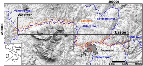
On this basis, and considering the need for an updated tool to guide future land planning in the Benevento Province, we use LiDAR data acquired in 2012 across the Benevento Province and discontinuous hydrometric data from 1924 to 2016 to produce a flood hazard map of its two major river segments. The first is the eastern, upper, segment of the Calore river starting approximately at the confluence with the Tammaro river and covering all of the industrial and urban areas of the town of Benevento (Figure 1(a)). The second is the western, lower, segment of the Calore river corresponding to the Telesina Valley, known for it’s high value agricultural production (Figure 1(b)). During the flood, the hydrometric stations located within the eastern and the western segments were destroyed, therefore, we made a comprehensive analysis of the flood in order to estimate its magnitude (i.e. fluvial stage) and associated return period.

Figure 1. Map showing major rivers of the Benevento Province (blue lines), western and eastern river segments object of the analysis (dark rectangles with labels) and cross sections (orange lines) used for the production of the digital elevation model of the water surface (wDEM). UTM 33 N coordinates are shown at the upper and left sides of the map.

2. Methods

Below, we describe the methods used to study the flood event of October 2015 and consequently develop the flood hazard map using high spatial resolution topography and probability analysis of hydrometric time series.

2.1. October 2015 event characterization

We used a post event Top of the Atmosphere (TOA) Sentinel 2 multispectral image taken on 15 November 2015 to map the area inundated by the flood. To recognize this area from the multispectral image, we used false color image composition (i.e. 11-8-3 bands, SWIR-NIR-Green, Figures 2(a,b)) and, since most of the floodplain is not covered by high vegetation, we computed the Normalized Difference Water Index (NDWI; e.g. McFeeters, 1996; Figures 2(c,d)).

Figure 2. False color image composition maps (11-8-3 channels) showing the area flooded by the October event (black polygon) along the (a) eastern and (b) western river segments and NDWI maps showing the flooded area (black/white polygon) of the same segments (c and d, respectively) of the Benevento Province. Yellow symbols indicate position and direction of taking of photos in Figure 3. See Figure 1 for map positions and extent.

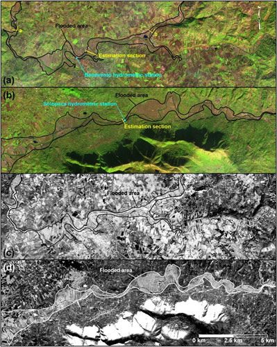
The NDWI is a satellite-derived index from the reflectance in green and Near-Infrared (NIR) channels that can be applied to delineate open water features and has the potential to distinguish flooded and non-flooded areas (Hudson & Colditz, 2003; Wang, Colby, & Mulcahy, 2002). Since it might not work properly under high vegetation that typically characterize fluvial shores, it is often used in combination with the NDVI index (e.g. Powell, Jakemam, & Croke, 2014). In this case, zones characterized by high vegetation are limited because most of the floodplain is used for cropping and due to the effect of the flood that removed most of the trees that colonize river embankments. Therefore, in this case the NDVI was not used.

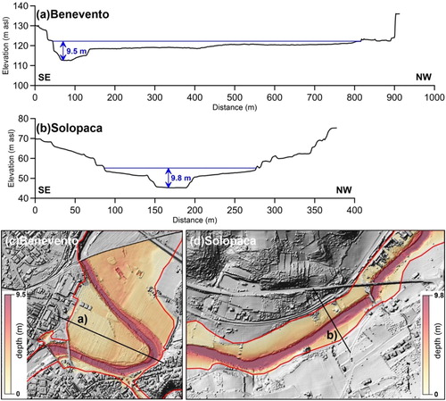
Once recognized through visual interpretation of the images, the inundated area was field validated considering the position of the geomorphologic signature of the flood on inactive fluvial scarps bounding river terraces and considering the photographic documentation acquired immediately after the event (e.g. Figures 3(a,b)). After validation, the mapped flooded area was used as boundary condition (target water level) to estimate water depth during the event next to the monitoring stations of Benevento and Solopaca. This estimation was completed through the reconstruction of the cross-sectional geometry of the floodplain and intersection of a line at the target water level and using lake analysis. Lake analysis was completed through the r.lake module implemented in GRASS GIS (e.g. Cannata & Marzocchi, 2012) over an area surrounding the monitoring stations. The r.lake module fills a lake to a target water level from a given starting point using as input data a raster map with at least one cell value greater than zero (e.g. https://grass.osgeo.org/grass72/manuals/r.lake.html). In this case, the input data for lake analysis was the LiDAR derived flood inundation map (See below for flood inundation map generation). The maximum relative elevation (i.e. water depth) above the river, estimated from cross sections (Figures 4(a,b)) and lakes (Figures 4(c,d)), was used as reference value for this event in the annual maxima hydrometric time series. We used probability analysis to estimate the theoretical return period of this event on the basis of available data and understand if it can be considered as the reference flood scenario for the Benevento Province according to the Garry and Graszk (1999) method. The theoretical return period was calculated as the inverse of the probability of exceedance.

Figure 3. Example of geomorphologic signature of the flood along the eastern river segment of the Benevento Province. The yellow dashed line indicates the boundary of the involved area. See Figure 2 for the position when taking the photo.

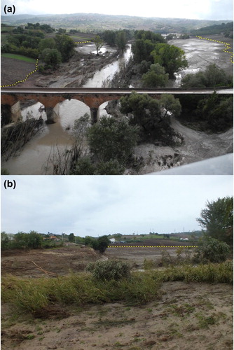
Figure 4. Water depth estimated considering the area flooded in October 2015. (a) and (b) report water depth estimation from cross-sectional geometry of the floodplain next to the Benevento and Solopaca instrumentation stations, respectively. (c) and (d) report water depth estimation from lake analysis next to the Benevento and Solopaca instrumentation stations, respectively. Cross section position is reported in figures (c) and (d) and Figure 2. Consider cross-sections length for scale reference in (c) and (d).

2.2. Flood inundation and hazard mapping

As a first step in deriving the flood hazard map, we compute a flood inundation map (i.e. relative elevation above the river) as a difference between a bare-earth, airborne LiDAR derived Digital Surface Model and a digital elevation model of the water surface (wDEM). The LiDAR DSM has a 2 × 2 m cell size and is resampled from a 1 × 1 m cell size using cubic convolution (e.g. Wu, Li, & Huang, 2008). The wDEM is computed through the interpolation of a triangulated irregular network of the water elevation data at cross-sections constructed along the river segments. Cross-section positions are consistently selected as function of the geometry of the river course, surrounding slopes and relative watershead (e.g. Cook & Merwade, 2009; Figure 1).

As a second step, we use a type III Generalized Extreme Value distribution function (GEV, ξ < 0; e.g. Hosking & Wallis, 1986) to fit the annual maxima time series (i.e. discontinuous complementary cumulative distribution function, CCDF; Figs (a, b, c, d, e and f) of the Main Map) registered at the Benevento and Solopaca hydrometric stations (see Figure 2 for position) between 1924 and 2016 and estimate the annual probability of exceedance (p) of each specific fluvial stage (x) in the range of interest and related return periods. The GEV function has the following form:(1) $F\left(x\right)=\exp \left\{-{\left[1+\xi \left(\frac{x-\mu }{\sigma }\right)\right]}^{-1/\xi }\right\}\mathrm{for}\xi \ne 0$(1) where ξ is the shape parameter, σ is the scale parameter and µ is the location parameter. As indicated by Coles (2001), the Generalized Extreme Value distribution function is suitable to describe the statistical behavior of annual maxima but has the disadvantage of underestimating the intensity of very high return period events. To overcome this drawback, we use it in combination with a Gamma distribution function (e.g. Yue, 2001) that has the potential to better estimate the intensity of very high return period events and has the following form:(2) $F\left(x\right)=\frac{{\beta }^{\alpha }{x}^{\alpha -1}{\mathrm{e}}^{-\beta x}}{\mathrm{\Gamma }\left(\alpha \right)}$(2)

where α is the shape parameter and β is the scale parameter and Γ(α) is the gamma function that is calculated as follow:(3) $\mathrm{\Gamma }\left(\alpha \right)={\int }_0^x{x}^{\alpha -1}{\mathrm{e}}^{-x}\mathrm{d}x$(3)

GEV and Gamma parameterization is automatically completed using the distribution fitter tool implemented in MATLAB (GEV Benevento: ξ = −0.168, σ = 1.740, µ = 3.415; GEV Solopaca: ξ = −0.153, σ = 1.765, µ = 3.752; Gamma Benevento α = 2.9812, β = 1.39506; Gamma Solopaca: α = 4.61855, β = 0.979929). Function combination is completed considering the univariate statistics of each time series. Especially, we use the GEV functions for inundation stages lower or equal to the time series 75^th percentile (5.23 m for the Benevento hydrometric station and 5.53 m for the Solopaca hydrometric station; Figures (b and e) of the Main Map) and the Gamma function for higher inundation stages. Since we have two time-series, the statistical analysis provides two specific GEV distribution functions and two specific Gamma distribution functions, a first pair for the eastern segment crossing the Benevento town (Benevento station) and a second pair for the western segment comprising most of the Telesina Valley (Solopaca station). Each pair is used to derive a composite fit for each station that is shown in the graphs c and f of the Main Map using the dashed red line.

In both cases, residual analysis indicates a very high goodness of fit for both functions (R² ≥ 0.99 for the GEV functions and R² ≥ 0.95 for the Gamma functions, see Figs. c and f in the Main Map). Even if the goodness of fit of the Gamma function is lower that the GEV function, the visual analysis of the graphs of figures c and f of the Main Map suggests the higher performances of the Gamma function at higher water stages. Additionally, a calculation of the RMSE between the measured and modeled fluvial stages (for the two stations and as function of the theoretical probability of exceedance) indicates that for higher stages, the RMSE of the GEV function is consistently higher than the RMSE of the Gamma function (e.g. considering the highest three stages: Benevento, GEV RMSE = 0.83, Gamma RMSE = 0.77, Solopaca, GEV RMSE = 1.04, Gamma RMSE = 0.69; considering the highest two stages: Benevento, GEV RMSE = 1.0, Gamma RMSE = 0.73, Solopaca, GEV RMSE = 1.26, Gamma RMSE = 0.65). The combined functions (GEV for x ≤  75th percentile and Gamma for x > 75th percentile) are used to derive the flood hazard maps from inundation maps as annual probability of exceedance maps (Main Map) and floodplain zonation maps (inset maps of the Main Map). Floodplain zonation is completed considering four zones, each corresponding to a specific hazard level. These zones are selected accordingly to the local Basin Authority guideline and considering the morphology of the floodplain. Especially, we identified a i) very high hazard zone that could be flooded as a consequence of 1 to 5 year floods, a ii) high hazard zone that could be flooded as a consequence of 5 to 30 year floods, a iii) medium hazard zone that could be flooded as a consequence of 30 to 100 year floods and a iv) low hazard zone that could be flooded as a consequence of 100 to 500 year floods. Flood magnitude for each specific return period is derived from probability analysis considering that the theoretical return period is the inverse of the probability of exceedance.

It is important to note that flood hazard estimation is completed using a simple elevation-based approach (e.g. Teng et al., 2017) that has the disadvantage of classifying, areas topographically disconnected from the river course and/or the flood plain, as floodable. This drawback would suggest that a preliminary identification of the area connected or connectable (e.g. area protected by river embankments) to the river is needed. Once identified, these areas can be manually removed from the model. Having said that, we do not exclude these areas from the analysis because even if they might not be directly flooded by the river outflow, they have the potential to be flooded due to secondary pluvial process like concentrated runoff or could be flooded in the case of embankment damage as in the event of October 2015. Thus, for the study area this represents a cautionary condition that might be considered as acceptable. Additionally, the flood inundation map is developed considering as an upper boundary the maximum stage of the river estimated for a 500 year flood. This is according to the Italian Basin Authorities guidelines.

Moreover, the flood inundation maps on which the hazard computation is based are not fully comparable (from the spatial viewpoint and considering its total extent) with any event-map. However, they are able to simulate or be reliable for different flooding scenarios of same magnitude but generated by different rainfall spatial distribution. This because the presented method is simpler than hydrodynamic models and only based on the relation between floodplain topography and fluvial stage. This makes the method able to work at both local and regional scale. A further simplification is that we do not consider the effect of climate change and channel adjustment that might influence the reliability of the analysis in the long-term (Magliulo, Valente, & Cartojan, 2013; Scorpio & Rosskopf, 2016; Whitfield, 2012).

3. The October 15th event and the extreme flood scenario

The flood was triggered by a storm that started on the night of 14 October and stopped on 15 October 2015, early in the morning. Data from the monitoring network of the Campania Region (http://www.agricoltura.regione.campania.it/meteo/rete.htm) indicated that a maximum cumulative rainfall value of ∼415 mm was recorded at the Paupisi meteorological station. More than 100 mm was recorded at 20 meteorological stations located within the Benevento Province in an area of about 2000 km². Approximately 50% of this area corresponds to the Tammaro river basin (∼800 km²). The destructive overflow hit the middle and lower course of the Tammaro river downstream from the Campolattaro dam and the middle and lower course of the Calore river that crosses the industrial area, the town of Benevento and the Telesina Valley (Figure 2). The flood involved an area across rivers floodplains of about 30 km² and was characterized by a maximum river stage of ∼9.8 m estimated next to the Solopaca station (Figure 4(b,d)). A water stage of ∼9.5 m was estimated within the town of Benevento (Figure 4(a,c)). In the industrial area of Benevento, next to the confluence between the Tammaro and the Calore rivers, all of the factories were damaged or completely destroyed. It was estimated that the flood caused about €1 billion worth of damage to local agriculture (Magliulo & Cusano, 2016).

Despite its socioeconomic impact, the probability analysis of available data indicates that this event has a theoretical return period of between 25 and 50 years (Solopaca and Benevento hydrometric stations, respectively; see gray stars in graphs c and f of the Main Map). Flooding events with return periods shorter than 100 years should not be considered as reference for hazard analysis even if they represent a well-known event that society wants to protect itself from (Garry & Graszk, 1999). Additionally, the guideline of the Italian Ministry of Environment and Land Protection underline that for hazard evaluation a 300 to 500 year event should be considered as extreme flood reference. For the analysis, we consider the 500 year flood and estimated its magnitude in terms of water depth using the combined function that for high intensity event uses the Gamma distribution function. It indicates that the 500 year event has an estimated magnitude of ∼13 m for the Solopaca hydrometric station (i.e. the western segment) and ∼14.5 m for the Benevento hydrometric station (i.e. the eastern segment; red stars in graphs c and f of the Main Map).

4. The flood hazard map

The Main Map reports the hazard maps derived from GIS processing and probability analysis. It is composed by the annual probability of exceedance maps and the hazard zonation maps (inset maps of the Main Map). The annual probability of exceedance maps for the major river segments of the Benevento Province are an interpretation of the hazard level across the Calore, Tammaro and Ufita floodplains connected to the occurrence of storm-induced floods of different magnitudes. These maps are simple tools suitable for identifying the hazard level of each human structure located within the floodplains on annual basis and is the first step toward a flood risk evaluation for this area. Being estimated on the basis of a flood inundation map (see methods section), the flood hazard tends to assume higher values for low values of the relative elevation above the river. It also varies as function of the distance from the river and the cross-sectional geometry of the river valley. In fact, where the river banks are sufficiently high, the hazard level evolves form very high (around 100% of probability), within or next to the river bed, to low values, across the adjoining floodplain. An example is the upper Telesina Valley where the river banks has a relative elevation up to 7.5 m.

The zonation maps (inset maps of the Main Map) show four zones of the floodplain that can be flooded by events of specific return period (see methods section). As indicated by the maps, most of the analysed floodplain is classified from very high to high hazard zones and the zones of medium and low hazard are poorly developed. It is important to notice that a part of the industrial zone, the western part of the Benevento town and the area located along the Sabato river are classified as very high to high hazard zones. In this context, the maps have the potential to support future land planning, guiding recommendation of uses, occupation restrictions and flood insurance plan development of the analysed floodplain segments (e.g. Linnenluecke & Griffiths, 2010). Additionally, since most of the existing protection embankments were surmounted and/or damaged by the October 2015 event, they should support the designing of new flood mitigation measures in terms of typology, position and geometry and the identification of zones of flood expansion for lamination purposes.

5. Conclusions

The hazard maps provide an overview of the flood hazard in the central sector of the Benevento Province which was hit by the flood event of October 2015. Representing the first step toward an evaluation of flood risk in the central sector of Benevento Province, they allow to estimate the specific hazard level for each human structure located across the floodplain of Calore (lower sector), Tammaro (a small part of its lower sector) and Ufita (a limited part of its lower sector) rivers and provide a zonation in flood perspective. Conversely from products that are based on hydrodynamic models of flood, these maps derive from statistical analysis of measured fluvial stage and LiDAR derived high-resolution topography which make them suitable to guide future land planning in an urban area like that of Benevento. In this way, the presented method has the potential to be applied in many fluvial contexts for which fluvial stage and topographic data are available and has no limitation to work at different scales, from local to regional. The resulting hazard maps, developed in direct collaboration with the Benevento Province authority, should be considered as a tool to support policy decision oriented to flood mitigation in the analysed floodplain segments (i.e. recommended uses, occupation restrictions and flood insurance plan development). Being a tool for preventing and reducing losses caused by floods, they also represent a contribution toward a better understanding of the environmental risk in this sector of the Benevento Province.

Software

The map was made using Golden Software Map Viewer 8. Hydrometric data were processed using Microsoft excel and Matlab^tm 2017 (https://it.mathworks.com/products/matlab.html). DEMs were generated and or modified using Quantum GIS, Open Source Geographic Information System, licensed under the GNU General Public License. Quantum GIS is an official project of the Open Source Geospatial Foundation (OSGeo, public domain software).

Acknowledgements

We thank Guy Schumann, Thomas Pingel and Karen Joyce, for their constructive reviews of the paper and Tommaso Piacentini for providing helpful editorial suggestions.

Disclosure statement

No potential conflict of interest was reported by the authors.

ORCID

Luigi Guerriero http://orcid.org/0000-0002-5837-5409

Francesco M. Guadagno http://orcid.org/0000-0001-5195-3758

Paola Revellino http://orcid.org/0000-0001-8303-8407

Additional information

Funding

This work was supported by the Benevento Province Authority.

References

- Alfonso, L., Mukolwem, M. M., & Di Baldassarre, G. (2016). Probabilistic flood maps to support decision-making: Mapping the value of information. Water Resources Research, 52, 1026–1043. doi: 10.1002/2015WR017378
- Andriola, L., Delmonaco, G., Margottini, C., Serafini, S., & Trocciola, A. (1996). Andamenti meteoclimatici ed eventi naturali estremi in Italia negli ultimi 1000 anni: alcune esperienze nell’ ENEA. Atti dei Convegni Lincei 129 su Eventi estremi: previsioni meteorologiche ed idrogeologia, Roma, 5 Giugno 1995, pp. 95–114.
- Barredo, J. I. (2009). Normalised flood losses in Europe: 1970–2006. Natural Hazards and Earth System Sciences, 9, 97–104. doi: 10.5194/nhess-9-97-2009
- Bates, P. D., & De Roo, A. P. J. (2000). A simple raster-based model for flood inundation simulation. Journal of Hydrology, 236, 54–77. doi: 10.1016/S0022-1694(00)00278-X
- Cannata, M., & Marzocchi, R. (2012). Two-dimensional dam break flooding simulation: A GIS-embedded approach. Natural Hazards, 61, 1143–1159. doi: 10.1007/s11069-011-9974-6
- Cardinali, M., Cipolla, F., Guzzetti, F., Lolli, O., Pagliacci, S., Reichenbach, P., … Tonelli, G. (1998). Catalogo delle informazioni sulle località italiane colpite da frane e da inondazioni. Progetto AVI, Pubblicazione CNR GNDCI n. 1799, v. 2.
- Cevasco, A., Diodato, N., Revellino, P., Fiorillo, F., Grelle, G., & Guadagno, F. M. (2015). Storminess and geo-hydrological events affecting small coastal basins in a terraced Mediterranean environment. Science of the Total Envionment, 532, 208–219. doi: 10.1016/j.scitotenv.2015.06.017
- Coles, S. (2001). An introduction to statistical modelling of extreme values. Springer series in statistics. London: Springer-Verlag. ISBN: 1-85233-459-2.
- Cook, A., & Merwade, V. (2009). Effect of topographic data, geometric configuration and modelling approach on flood inundation mapping. Journal of Hydrology, 377, 131–142. doi: 10.1016/j.jhydrol.2009.08.015
- Di Baldassarre, G., Schumann, G., Bates, P. D., Freer, J. E., & Beven, K. J. (2010). Flood-plain mapping: A critical discussion of deterministic and probabilistic approaches. Hydrological Science Journal, 55, 364–376. doi: 10.1080/02626661003683389
- Di Martire, D., De Rosa, M., Pesce, V., Santangelo, M. A., & Calcaterra, D. (2012). Landslide hazard and land management in high-density urban areas of Campania region, Italy. Natural Hazards and Earth System Sciences, 12, 905–926. doi: 10.5194/nhess-12-905-2012
- Diodato, N. (1999). Ricostruzione storica di eventi naturali estremi a carattere idrometeorologico nel Sannio beneventano dal medioevo al 1998. Bollettino Geofisico a. XXII, n. 3–4.
- Diodato, N. (2007). Climatic fluctuations in southern Italy since the 17th century: Reconstruction with precipitation records at Benevento. Climatic Change, 80, 411–431. doi: 10.1007/s10584-006-9119-1
- Diodato, N., de Vente, J., Bellocchi, G., Guerriero, L., Soriano, M., Fiorillo, F., … Guadagno, F. M. (2015). Estimating long-term sediment export using a seasonal rainfall-dependent hydrological model in the Glonn River basin. Germany. Geomorphology, 228, 628–636. doi: 10.1016/j.geomorph.2014.10.011
- Diodato, N., Guerriero, L., Fiorillo, F., Esposito, L., Revellino, P., Grelle, G., & Guadagno, F. M. (2014). Predicting monthly spring discharge using a simple statistical model. Water Resources Management, 28, 969–978. doi: 10.1007/s11269-014-0527-0
- Furdada, G., Calderón, L. E., & Marqués, M. A. (2008). Flood hazard map of La Trinidad (NW Nicaragua). Method and results. Natural Hazards, 45, 183–195. doi: 10.1007/s11069-007-9156-8
- Garry, G., & Graszk, E. (1999). Plans de prévention des risques naturels (PPR) : risques d’inondation, Guide méthodologique. Ministère de l’Aménagement du Territoire et de l’Environnement, Ministère de l’Équipement, Documentation Française, Paris, 123 pp.
- Gonçalves, P., Marafuz, I., & Gomes, A. (2015). Flood hazard, Santa Cruz do Bispo Sector, Leça River, Portugal: A methodological contribution to improve land use planning. Journal of Maps, 11, 760–771. doi: 10.1080/17445647.2014.974226
- Grelle, G., Soriano, M., Revellino, P., Guerriero, L., Anderson, M. G., Diambra, A., … Guadagno, F. M. (2014). Space–time prediction of rainfall-induced shallow landslides through a combined probabilistic/deterministic approach, optimized for initial water table conditions. Bulletin of Engineering Geology and the Environment, 73, 877–890. doi: 10.1007/s10064-013-0546-8
- Groisman, P. Y., Knight, R. W., Easterling, D. R., Karl, T. R., Hegerl, G. C., & Razuvaev, V. N. (2005). Trends in intense precipitation in the climate record. Journal of Climate, 18, 1343–1367. doi: 10.1175/JCLI3339.1
- Guerriero, L., Bertello, L., Cardozo, N., Berti, M., Grelle, G., & Revellino, P. (2017). Unsteady sediment discharge in earth flows: A case study from the Mount Pizzuto earth flow, southern Italy. Geomorphology, 295, 260–284. doi: 10.1016/j.geomorph.2017.07.011
- Guerriero, L., Diodato, N., Fiorillo, F., Revellino, P., Grelle, G., & Guadagno, F. M. (2015). Reconstruction of long-term earth-flow activity using a hydro-climatological model. Natural Hazards, 77, 1–15. doi: 10.1007/s11069-014-1578-5
- Guerriero, L., Revellino, P., Luongo, A., Focareta, M., Grelle, G., & Guadagno, F. M. (2016). The mount Pizzuto earth flow: Deformational pattern and recent thrusting evolution. Journal of Maps, 12, 1187–1194. doi: 10.1080/17445647.2016.1145150
- Hosking, J. R. M., & Wallis, J. R. (1986). The value of historical data in flood frequency analysis. Water Resources Research, 22, 1606–1612. doi: 10.1029/WR022i011p01606
- Hudson, P. F., & Colditz, R. R. (2003). Flood delineation in a large and complex alluvial valley, lower PáNuco basin, Mexico. Journal of Hydrology, 280, 229–245. doi: 10.1016/S0022-1694(03)00227-0
- Jongman, B., Ward, P. J., & Aerts, J. C. J. H. (2012). Global exposure to river and coastal flooding: Long term trends and changes. Global Environmental Change, 22, 823–835. doi: 10.1016/j.gloenvcha.2012.07.004
- Knox, J. C. (1993). Large increase in flood magnitude in response to modest changes in climate. Nature, 361, 430–432. doi: 10.1038/361430a0
- Linnenluecke, M., & Griffiths, A. (2010). Beyond adaptation: Resilience for business in light of climate change and weather extremes. Business & Society, 49, 477–511. doi: 10.1177/0007650310368814
- Magliulo, P., & Cusano, A. (2016). Geomorphology of the Calore river alluvial plain. Journal of Maps, 12, 1119–1127. doi: 10.1080/17445647.2015.1132277
- Magliulo, P., & Valente, A. (2014). Mapping direct and indirect fluvial hazard in the Middle Calore River valley (southern Italy). International Conference “Analysis and Management of Changing Risks for Natural Hazards”, Padua, Italy.
- Magliulo, P., Valente, A., & Cartojan, E. (2013). Recent geomorphological changes of the middle and lower Calore River (Campania, Southern Italy). Environmental Earth Sciences, 70, 2785–2805. doi: 10.1007/s12665-013-2337-8
- Maresca, R., Castellano, M., De Matteis, R., Saccorotti, G., & Vaccariello, P. (2003). Local site effects in the town of Benevento (Italy) from noise measurements. Pure and Applied Geophysics, 160, 1745–1764. doi: 10.1007/s00024-003-2376-2
- McFeeters, S. K. (1996). The use of the normalized difference water index (NDWI) in the delineation of open water features. International Journal of Remote Sensing, 17, 1425–1432. doi: 10.1080/01431169608948714
- Montané, A., Buffin-Bélanger, T., Vinet, F., & Vento, O. (2017). Mapping extreme floods with numerical floodplain models (NFM) in France. Applied Geogrphy, 80, 15–22. doi: 10.1016/j.apgeog.2017.01.002
- Nuswantoro, R., Diermanse, F., & Molkenthin, F. (2016). Probabilistic flood hazard maps for Jakarta derived from a stochastic rain-storm generator. Jounal of Flood Risk Management, 9, 105–124. doi: 10.1111/jfr3.12114
- Peduzzi, P., Dao, H., Herold, C., & Mouton, F. (2009). Assessing global exposure and vulnerability towards natural hazards: The disaster risk index. Natural Hazards and Earth System Sciences, 9, 1149–1159. doi: 10.5194/nhess-9-1149-2009
- Piacentini, T., Urbano, T., Sciarra, M., Schipani, I., & Miccadei, E. (2016). Geomorphology of the floodplain at the confluence of the Aventino and Sangro rivers (Abruzzo, Central Italy). Journal of Maps, 12, 443–461. doi: 10.1080/17445647.2015.1036139
- Powell, S. J., Jakemam, A., & Croke, B. (2014). Can NDVI response indicate the effective flood extent in macrophyte dominated floodplain? Ecological Indicators, 45, 486–493. doi: 10.1016/j.ecolind.2014.05.009
- Revellino, P., Grelle, G., Donnarumma, A., & Guadagno, F. M. (2010). Structurally-controlled earth flows of the Benevento Province (Southern Italy). Bulletin of Engineering Geology and the Environment, 69, 487–500. doi: 10.1007/s10064-010-0288-9
- Rossi, F., & Villani, P. (1994). Valutazione delle piene in Campania. Rapporto Regionale Campania, CNR-GNDCI.
- Scorpio, V., & Rosskopf, C. M. (2016). Channel adjustments in a Mediterranean river over the last 150 years in the context of anthropic and natural controls. Geomorphology, 275, 90–104. doi: 10.1016/j.geomorph.2016.09.017
- Sutcliffe, J. V. (1987). The use of historical records in flood frequency analysis. Journal of Hydrology, 96, 159–171. doi: 10.1016/0022-1694(87)90150-8
- Teng, J., Jakeman, A. J., Vaze, J., Croke, B. F. W., Dutta, D., & Kim, S. (2017). Flood inundation modelling: A review of methods, recent advances and uncertainty analysis. Environmental Modelling and Software, 90, 201–216. doi: 10.1016/j.envsoft.2017.01.006
- Toda, L. L., Yokingco, J. C. E., Paringit, E. C., & Lascoad, R. D. (2017). A LiDAR-based flood modelling approach for mapping rice cultivation areas in Apalit, Pampanga. Applied Geography, 80, 34–47. doi: 10.1016/j.apgeog.2016.12.020
- Wang, Y., Colby, J. D., & Mulcahy, K. A. (2002). An efficient method for mapping flood extent in a coastal floodplain using Landsat TM and DEM data. International Journal of Remote Sensing, 23, 3681–3696. doi: 10.1080/01431160110114484
- Whitfield, P. (2012). Floods in future climates: A review. Journal of Flood Risk Management, 5, 336–365. doi: 10.1111/j.1753-318X.2012.01150.x
- Woo, M., & Waylen, P. R. (1986). Probability studies of floods. Applied Geography, 6, 185–195. doi: 10.1016/0143-6228(86)90001-9
- Wu, S., Li, J., & Huang, G. H. (2008). A study on DEM-derived primary topographic attributes for hydrologic applications: Sensitivity to elevation data resolution. Applied Geography, 28, 210–223. doi: 10.1016/j.apgeog.2008.02.006
- Yue, S. (2001). A bivariate gamma distribution for use in multivariate flood frequency analysis. Hydrological Processes, 15, 1033–1045. doi: 10.1002/hyp.259
- Zazo, A. (1949). Lo straripamento del fiume Calore in Benevento nel 1740 e nel 1770. Samnium, a. XXII, n. 3–4, Benevento, p. 212.