Geovisualization geoscience of large river floodplains

ABSTRACT

Alluvial river landscapes of the lower Mississippi and Atchafalaya rivers in the south-central USA are flood prone and have shifted historically in position and form, resulting in interventions for flood reduction, navigation, and water supply. Fisk mapped these landscapes in the middle of the twentieth century as a series of artistic colourful map plates. Selected areas are revisited with modern data sets (LiDAR from 2003, hydrographic surveys from 2006 and 2007) including two sites along the Mississippi River (near the Old River juncture and near Morganza Floodway) and one in the middle Atchafalaya River. By using 2D and 3D geovisualization, we find that the extent, variety, and dimensions of anthropogenic landforms have grown in prominence since Fisk’s mapping. The volumes of the highest positive landforms are quantified to provide some indication of direct and indirect anthropogenic activity in these landscapes.

KEYWORDS:

• Geovisualization
• river mapping
• fluvial landscapes
• geomorphology
• anthropogenic landforms
• Mississippi River
• Atchafalaya River
• hypsometric tinting

1. Introduction

Early geological reports of the lower Mississippi and Atchafalaya rivers in the south-central USA (Fisk, 1944, 1952) included colourful map plates of historical channel courses, highlighting shifts of entire meander belts and formation of natural and artificial meander bend cutoffs. Created by a team (see LeBlanc, 1996; Robinson, 1996), the 1944 report uses a combination of colour and pattern to show the channel position during four exact dates (1944, 1880, 1820, and 1765) and 16 earlier times, as interpreted by relative dating using cross-cutting relationships of river channel segments reconstructed from aerial photographs (Figure 1). The Fisk (1952) report entitled ‘Geological investigation of the Atchafalaya Basin and the problem of Mississippi River diversion’ informed engineers and other readers that the ‘prospect of the Mississippi River being diverted into a shorter channel to the sea is not unique’, and explained that this is the normal process by which the Mississippi River has shifted its course in the past several thousand years. Coupled with the potential consequences of such a diversion, which would lead to the demise of ports and fresh water resources in New Orleans and Baton Rouge, the 1952 study inspired the need for an engineering solution known as the Old River Control Project. This project was completed in 1963, and has since been upgraded with additional structures as required (Mossa, 2013).

Figure 1. Sheet 13 (Plate 22) of the ‘Ancient Courses Mississippi River Meander Belt’ published by Fisk (1944). The legend in the top right corner shows the colour and pattern choice used by Fisk to present historical river courses (Source: Richards, unknown date).

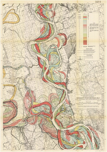
At a conference in 1994 to honour Fisk’s legacy, the river mapping work was described by former colleagues and assistants (Krinitzsky, 1996; LeBlanc, 1996; Robinson, 1996; Saucier, 1996) as being helpful for solving problems regarding flooding in the lower Mississippi valley, keeping the river navigable, minimizing the amount of bank erosion, locating sources of aggregate, groundwater and wetlands management, selecting optimum sites for foundations, and better understanding of fluvial systems. Although Saucier (1996) recognized many positive aspects of Fisk’s geological work, he also had criticisms, suggesting that the chronological reconstruction could be improved with better understanding of complexity, and with the use of radiocarbon and other numerical dating techniques for more precise age control, supplemented by archaeology for relative dating. Indeed, Fisk’s (1944) maps have a large measure of assumption, evenly dividing the 16 other stages in intervals of 100 years and combining the cross-cutting relationships of the various channel traces and scars (Figure 1) with approximate rates of known migration since 1765. The most recent stages are depicted in pastel solid colours, earlier historical courses are shown as varied patterns comprising a single colour for sets of four courses, and the earliest courses are patterned combinations of colours (Figure 1). Nonetheless, because of the calibre of creative craftsmanship these maps are featured prominently on the website ‘Radical Cartography’ (Rankin, 2017) and revered by many people. Morris (2015) explains:

So eye-catching are Fisk’s images that they have become web site back grounds, computer screen savers, and dorm room posters. They have inspired artists and informed conservationists, both of whom see in the images an organic or natural river that transcends or defies human engineering.

Dating back to Renaissance time, mapmaking and landscape painting were often performed by artists or craftsmen. This led to products such as the Map of Northern Tuscany and the Imola map by Leonardo da Vinci, which showed aerial views of river landscapes that blended ‘the pictorial and the planimetric, image and measurement’ (Rees, 1980). The Imola map uses colour to depict relative elevation, as well as water features and meandering river landforms such as sand bars, meander scrolls and cut banks. Furthermore, the map depicts anthropogenic alterations of the river, including irrigation canals and a water diversion used to build a protective moat (see Imhof, 1982 and map collection in Bambach, 2003).

Mapping technologies have advanced considerably in the 75 years since Fisk’s report, particularly in the past few decades. Indeed, other researchers are combining these new technologies to integrate colourful mapping with geoscience goals. Examples include mapping of spillage features on large floodplains (e.g. see Figure 8 of Lewin, Ashworth, & Strick, 2017) and the depiction of delta plain channel belt activity and geomorphic features (e.g. Figures 1; 4 and 5 of Pierik, Stouthamer, & Cohen, 2017). Another example of artful mapping with geoscience analysis focuses on evaluating the completeness of the sedimentary record in a modelled floodplain, the modern Mississippi River, and the Early Cretaceous McMurray Formation in Alberta, Canada (Durkin, Hubbard, Holbrook, & Boyd, 2018). Gaps in the geological record have been evaluated from Fisk’s (1944) maps, taken at face value, near New Madrid, Missouri, and supported by enhancement of Fisk’s maps (Figures 6 and 11 in Durkin et al., 2018) to show progressive decreases in preservation of accretion packages, bars, and meander belts from 100% at stage 1 to between 10% and 20% at Stage 16.

In this paper, our aim is to re-examine the Mississippi and Atchafalaya rivers using Light Detection and Ranging (LiDAR) data as well as other topographic and hydrographic data (e.g. from the United States Geological Survey, US Army Corps, field surveys) for depicting landscapes. We combine these data with modern 2D and 3D mapping supported by hillshade relief (Biland & Çöltekin, 2017; Imhof, 1982; Kennelly, 2008; Marston & Jenny, 2015), texture, stylization, pattern (Bratkova, Shirley, & Thompson, 2009; Christophe et al., 2016) and colour scheme design (Patterson, 2001). Scientific visualization can be an important tool for analysis and communication (Mitasova, Harmon, Weaver, Lyons, & Overton, 2012) but so far these lowland alluvial rivers that are critical to the US economy for navigation, flood control and industry, and that also form the basis for many fundamental concepts in fluvial and anthropogenic geomorphology, have not been examined with geovisualizations.

Since Fisk (1944, 1952), these rivers and their floodplains have had additional engineered diversions and other positive and negative landforms of anthropogenic origin that were created to support improved navigation, control floods, and to extract resources. Our research uses unique colour scheme designs and 3D visualization with Geographic Information Systems (GIS) and the interactive ArcGIS Online CityEngine Web Viewer. By merging different sources, such as LiDAR and hydrographic surveys, using vertical exaggeration, and selecting colour schemes, these maps and related visualizations depict spatial variations in underwater topography, accentuate low-relief and artificial landforms, and contrast active and abandoned channels. Thus, these maps and visualizations have potential to educate the public and scientific community about issues at these specific sites such as altered longitudinal and lateral connectivity, needs for landscape and river restoration, and likely impacts of similar projects in the developing world.

2. Site selection and study area background

We chose to depict the landscapes of two large alluvial rivers (Mississippi 3.2 × 10⁶km²; Atchafalaya > 0.17 × 10⁶km²) at three sites that include structural modification for floods, and a mixture of natural and artificial landforms (Figure 2).

Figure 2. Map of the study area with each area of interest (AOI) in southeastern Louisiana: Old River area, Morganza Floodway area, and Atchafalaya River.

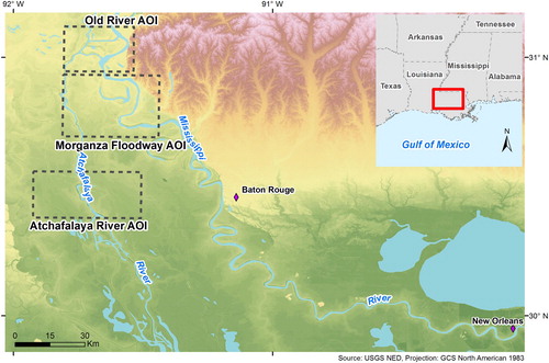
The first site is the juncture of the Mississippi and Atchafalaya at Old River, located approximately 490 km (river mile 305) AHP (above the Head of Passes) where flow divides into several channels at the bird-foot delta. The area of interest (AOI) is about 25 × 20 km (Figure 2). Here, the rivers were disconnected by a cutoff made by Captain Shreve in 1831, then joined for several decades by a canal that was maintained by dredging until 1937 (Mossa, 2013). As the Atchafalaya started receiving more flow, Fisk’s studies suggested the need for engineering control to regulate flow near this juncture. Currently, ∼30% of the Mississippi River flow is diverted into the Atchafalaya near this sparsely populated site. In 1963, there was one diversion and by 1990 there were three. The east side of the river is partially bordered by an artificial levee due to the hilly topography where the river abuts the valley wall. Artificial levees surround the floodplain channels because control of the river here is essential for maintaining the Mississippi River in its current course; if the course were to be diverted, the cities of New Orleans and Baton Rouge would quickly lose their fresh water and importance for navigation.

The second site is the juncture of the Mississippi River with the Morganza Floodway at 450 km (river mile 280) AHP (Figure 2). The AOI is about 35 × 25 km. First proposed following the flood of 1927, the structure was not completed until 1954, although levees were present much earlier. Nearby, there is a large oxbow lake known as Raccourci Old River, which connects to the Mississippi through a tie channel (Rowland, Dietrich, Day, & Parker, 2009; Rowland, Lepper, Dietrich, Wilson, & Sheldon, 2005). As upriver, the area is rural but human imprint is evident. Opened during the 1973 and 2011 floods, the purpose of the floodway and adjacent levees is to divert floodwaters upstream of the more populated (e.g. Baton Rouge and New Orleans) sections of the lowermost Mississippi River to the Atchafalaya basin.

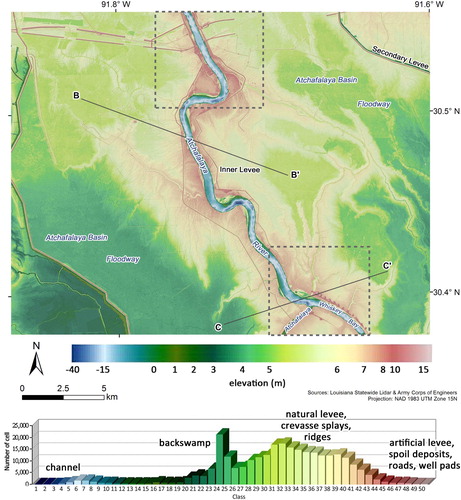
The third site is in the middle Atchafalaya River near 88 km (river mile 55), as measured from the former connection with lower Old River (Figure 2). The AOI is about 40 × 20 km. As with the other sites, this rural site shows varied natural features with a human overprint. The Atchafalaya River is much narrower than the Mississippi, but has two sets of levees: an inner set which ends near this location, and an outer set that forms the Atchafalaya basin floodway. This river has increased considerably in width, cross-sectional area and flow since an ∼50 km (30 mile) long log jam was burned and busted by the state of Louisiana in the 1880s (Mossa, 2016; Reuss, 2004). Due to its shorter distance to the Gulf of Mexico, avulsion of the Mississippi into this shorter and steeper course was anticipated and prevented by engineering intervention that regulated flow at the Old River juncture.

3. Methods

In this study, LiDAR data and hydrographic maps were acquired and combined into continuous elevation surface models for mapping. The Louisiana state-wide LiDAR project does not include underwater elevations (Cunningham, Gisclair, & Craig, 2003), so the closest date of the hydrographic survey from the Army Corps of Engineers (U.S. Army Corps of Engineer New Orleans District, 2009; U.S. Army Corps of Engineers New Orleans District, unpublished) was combined with the LiDAR data. The artificial levee feature layer was also obtained (Table 1).

Table 1. Details of data and maps applied in this study.

Data	Date/Source	Scale/Resolution	Format
Fisk Channel	Fisk, 1944	1:63300 (scanned file)	GeoTIFF
LiDAR points	Louisiana Statewide Lidar, Feb. 2003	Point spacing less than 3–4 m, point clouds has been edited to ground-only points	comma-separated values (CSV)
Hydrographical survey	Army Corps of Engineers, 2006 and 2007	1:10,000	design file (DGN)
Levee shapefile	Army Corps of Engineers, 2006	N/A	shapefile (.shp)

3.1. Combining LiDAR data and hydrographic maps

In order to combine LiDAR data and hydrographic survey maps in terrain models, interpolation surfaces were created, based on the hydrographic survey points. Random points with a similar density to the LiDAR data (3–4 points per m²) were then generated to extract values from the interpolation surfaces. Both the original survey points and the generated random points were imported into terrain models in AOIs. The LiDAR-edited points were also imported into terrain models to create a continuous river-land elevation surface model with 1 m resolution.

3.2. Designing and applying colour schemes

Several methods can be used to apply hypsometric tinting to elevation models. Here, we focused on cell value classification and hypsometric tinting design. Uplands in AOIs were first masked out to better emphasize the floodplains. Four common classification methods were applied to determine which classification presented better details of floodplain features with 50 classification intervals: equal interval, quantile (equal count), natural break (Jenks algorithm), and geometrical interval methods.

The equal interval method simply splits cell values from minimum to maximum into 50 equal intervals. The quantile method is based on the total number of cells divided by 50 classes, and so each class has, theoretically, the same number of cells. The natural break method is based on the method discussed in Jenks and Caspall (1971), and calculates the relationship between each value and nearby two classes, and reassigns the value to reach a final classification with higher similarity of values within each class. The geometrical interval method is based on geometric series with the purpose of creating a classification that has both similar values within each class and reasonable change of values in all the classes, and aims to work with data not normally distributed (ESRI, 2007; Slocum, 1999; Smith, Goodchild, & Longley, 2015). Results from different classification methods were applied with hypsometric tinting to get initial maps of classification results. Maps for AOIs and histograms for each classification were created for visualization. The decision of classification selections was based on the distribution of colours, and appearance of river channel and floodplain features.

Once the classification method was chosen, colour schemes were designed for each AOI. Generally speaking, the colour scheme was selected based on the reader’s association of colours (Chen, Zick, & Benjamin, 2016; Imhof, 1982; Slocum, 1999). For elevation models, colour selection was associated with natural landscapes (Imhof, 1982), such as blue for water, green for forest, and white for snow on the top of mountains. For instance, the default colour scheme in ArcMap (Elevation #1, Elevation #2, and Surface) combines these natural colours. These default schemes work well for areas of high elevation relief but do not suit floodplain areas. Here, colour schemes were specifically designed for floodplain features with multi-part colour ramps. Each multi-part colour ramp was combined with 10 colour changes. The colours were selected based on the land cover and number of cells. The lowest area was mostly river channel and so dark blue and light blue were selected in these colour ramps; in the areas elevated above the river, colours were chosen from blue-green for lower floodplain elevations, yellow-green to green for mid floodplain elevations, and sandy-pinkish colour for the higher floodplain elevations to get a better contrast. For the highest areas, bright red and grey colours were chosen for artificial levee, road networks, and uplands.

Hillshade effects were also applied to present floodplain features. Two hillshade layers were created with 1 and 10 times vertical exaggeration. The 10 times vertical exaggeration layer was assigned 75% transparency and overlap with the 1 time vertical exaggeration for presentation aesthetics adopted by Coe (2016). Both hillshade layers were overlain with the elevation model layer with 35% transparency on the top.

3.3. Creating 3D models

3D models were also built to demonstrate a different perspective for floodplain features. A 3D interactive online model was created for each AOI by using ArcScene and CityEngine Web Scenes. In ArcScene, elevation models and the levee shapefile were imported and assigned designed colour schemes. The vertical exaggeration was set as 10 times to better visualize low-relief landforms. ArcScene map documents were then saved and converted to web scene files. In the ESRI CityEngine Web Scenes website (https://www.arcgis.com/apps/CEWebViewer/viewer.html), files were uploaded and descriptions and comments edited on the introduction pages. Additionally, at a few locations, feature areas and volumes were extracted above local arbitrary elevations to quantify the role of humans in altering the landscape.

4. Results

4.1. Classification of elevation values

Four classification methods were applied to classify elevation values (Figure 3). Perhaps the easiest to understand is the equal interval method, which is not suitable for a highly skewed distribution of elevation values, so most of the floodplain was classified in a narrow colour range (Figure 3(A,A’)). The quantile method, on the other hand, was applied in an attempt to evenly distribute elevation values to each class but failed because of the highly skewed distribution of elevation values (ESRI, 2017). Nevertheless, it created a fairly even distribution across the range of elevations (Figure 3(B,B’)). The natural break method result was similar to the equal interval method owing to the highly skewed distribution, because the algorithm reassigned values according to the alongside classes. It created a slightly better distribution than the equal interval method but was still affected by the high number of values in few classes (Figure 3(C,C’)).

Figure 3. The cell value distributions and result maps for four classification methods. Here, Old River AOI is selected to demonstrate a variety of landforms and landscapes with different classification methods. In A through D, the y axis is the class number, and the x axis is the number of cells.

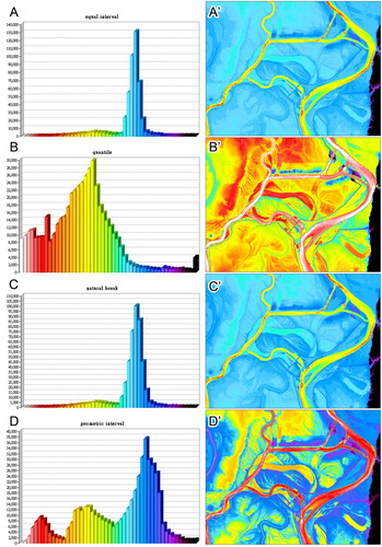
The geometrical interval method produced the most even distribution. With this method, the river bathymetry was more differentiated from other land covers and landscapes (Figure 3(D,D’)). It also distinguished the upper floodplain of the Mississippi River and the lower floodplain of the Atchafalaya River. In general, the geometrical interval method offered more differentiation of the river bathymetry and floodplain, and more even distribution in colour classes, which is preferred for our goal of identifying distinctive topographic features. As such, the geometrical classification method was selected for colour scheme design and mapping.

4.2. Colour scheme design and 3D webscene

The overview maps and 50 level classifications for each AOI are shown in Figure 4 and Main Map (Old River AOI), Figure 5 and Main Map (Morganza Floodway AOI), and Figure 6 and Main Map (Atchafalaya River AOI), with some floodplain features noted on the figures. Due to the relatively low density of data points in the hydrographic surveys from 2006, the bathymetries of Mississippi River and Atchafalaya River, and especially Raccourci Old River, have coarser resolution compared with the LiDAR DEM (Digital Elevation Model), but they show undulating bed variations such as pool and riffles (pools are deep and often coincide with the outer edge of a meander bend, whereas riffles are shallower areas between bends), scour zones (areas of the riverbed locally deepened by floods, shown in darker blues as in the Old River channels), and zones of lake sedimentation Figures 4–6, Main Map). Within the floodplains, the pink and red colours comprise high relative elevation anthropogenic features such as the artificial levee and road networks, and natural features such as the higher portions of natural levees, crevasse splays, fans at the edge of uplands, and stream valleys within uplands (Figures 4–6, Main Map).

Figure 4. Landscapes and landforms of Old River AOI are discernible from coupled LiDAR-bathymetric data using a 50-class colour scheme design. Dashed rectangles indicate zoom in areas shown in Figure 8(A,B) and the solid line denotes the A-A’ profile shown in Figure 11.

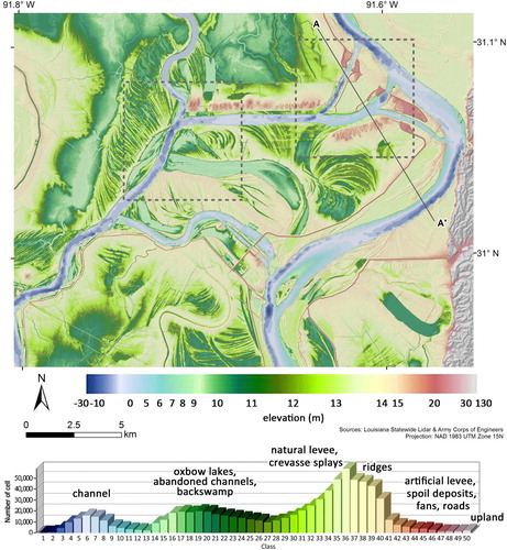
Figure 5. Landscapes and landforms of the Morganza Floodway AOI are discernible from coupled LiDAR-bathymetric data using a 50-class colour scheme design. Dashed rectangle indicates zoom in area shown in Figure 8(C).

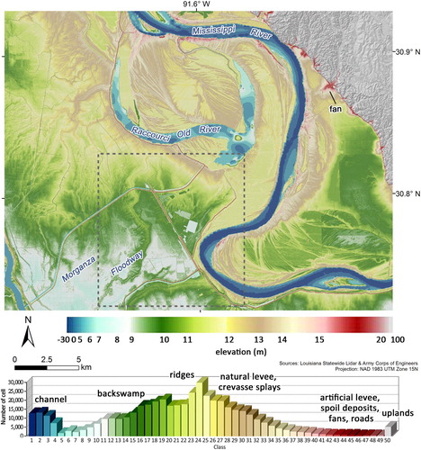
Figure 6. Landscapes and landforms of the middle Atchafalaya River AOI are discernible from coupled LiDAR-bathymetric data using a 50-class colour scheme design. Dashed rectangle indicates zoom in areas shown in Figure 9(A,B) and the solid lines denote the B-B’ and C-C’ profiles in shown Figure 11.

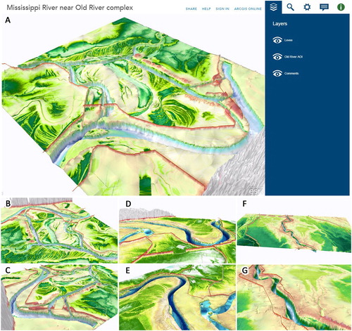
Figure 7 shows snap shots of website and 3D models. Users can rotate/shift the elevation models and turn levee layers on and off, switch to different views to observe the variety of floodplain features, and make snap shots. Direct links to the 3D models for each AOI are:

Mississippi River at the Old River complex (https://arcg.is/1uK0q), Mississippi River at Morganza Floodway (https://arcg.is/0fuHaP0), and the middle Atchafalaya River and Floodway AOI (https://arcg.is/1yuSSj)

Figure 7. 3D model snapshots from CityEngine Web Scenes: (A), (B), (C) Old River AOI; (D), (E) Morganza Floodway AOI; and (F), (G) Atchafalaya River AOI.

4.3. Geoscience learning and comparison with fisk’s channel change maps

From a geoscience perspective, these 2D and 3D maps show features and phenomena not presented on Fisk’s (1944) maps (Table 2; Figures 4–9, Main Map). A variety of natural landforms and landscape scenes are manifest in each of the different AOIs (Table 2). Additionally, some comparisons between different rivers and with Fisk’s (1944) maps can be used to enhance geoscience learning. Some of the landforms observed are natural features associated with alluvial rivers and others include a variety of artificial landforms (Szabó, 2010), many of which have clear, closed boundaries while others are somewhat fuzzy (Evans, 2012). Besides artificial levees, other anthropogenic features can be observed, including positive landforms such as elevated roads and highways, railroads, spoil mounds, agricultural fence or vegetative boundaries, and well pads for oil drilling (Figures 8(A,B) and 9). Due to the abundant wetlands in the area, nearly all artificial landforms are built from fill, typically either using sand, gravel, or shell brought in from elsewhere, or local sediments. Borrow pits (linear depressions in the floodplain where sediments are extracted) are a common negative landform in this setting, as they provide local fill for making artificial levees and roads. The highest relief negative landforms are the rivers, including the anthropogenic artificial inflow and outflow channels of the Old River diversion complex (Figures 4 and 7(A–C), Main Map). Another negative relief anthropogenic feature is the rectangular fields that are lower than the surrounding areas; for instance, near the entrance to the Morganza Floodway (Figures 5 and 8(C), Main Map). Most likely, these are lower because these wetland fields were drained and have since subsided relative to the surrounding terrain.

Figure 8. Comparison of combined LiDAR and hydrographic survey DEM (∼2007 data) with parts of Fisk’s (1944) historical channel change maps.

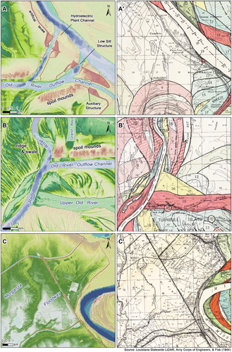
Table 2. Geoscience learning from 2D and 3D renditions of the study area.

Site/Related Figures	Features and phenomena observed in 2D and 3D models
Old River (Figures 4, 7 and 8, Main Map, 3D link)	Scour zones in Old River Low Sill Channel where the structure was heavily damaged during the flood of 1973
	The geometry of the natural channels as compared with the varied artificial Old River inflow and outflow channels
	Dredge spoil, runny or reworked by floods
	Increased sedimentation/elevation inside levee boundaries or batture
	Relative elevations of active (Old River Outflow Channel), controlled (Old River navigation channel) and abandoned (Upper Old River) channels at junctures with the Red and Atchafalaya Rivers
Morganza (Figures 5, 7 and 8, Main Map, 3D link)	Alluvial and colluvial fans (Smith, 1996) at foot of upland
	Spatial variability in lake sedimentation of Raccouri Old River, an artificial cutoff formed in 1848
	The intersection of natural features (crevasse splays) with artificial ones (constructed levees)
Middle Atchafalaya (Figures 6 and 7, 9, Main Map, 3D link)	Sedimentation confined within both inner and outer levees as shown by differences in relative elevations
	Crevasses protruding onto backswamp
All (Figures 4–9, Main Map, 3D links)	Transition from natural levee to backswamp with increasing distance from the river
	Riffles and pools (bed variations) evident in large alluvial rivers
	Agricultural fields create subtle lines and polygons due to fences, vegetation placement, and subsidence associated with wetland drainage
	Dependence of south Louisiana on levees and structural mitigation
	Linear borrow areas (canals and long lakes) adjacent to artificial levees
	Other anthropogenic features including roads, railroads, spoil mounds, and well pads show higher relief than most natural features, impacting water flow and connectivity
Comparisons (Figures 3–8, Main Map, 3D links)	Between Mississippi and Atchafalaya: the older and historically more laterally active Mississippi River shows more extensive ridge and swale topography and abandoned channels
	Between Mississippi and Atchafalaya: dredge spoil mounds appear different from each other and differ in form from Apalachicola River (Mossa, Chen, Walls, Kondolf, & Wu, 2017), possibly due to reworking by floods and/or finer sediment in Mississippi
	Between Fisk and this paper: Fisk’s artistic paleochannels sometimes don’t match well with LiDAR
	Between Fisk and this paper: The anthropogenic imprint has become more dominant on this landscape since Fisk

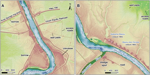
3D and interactive views give insights different to those gained from 2D maps. For instance, the relative elevations of the varying active and abandoned channels entering the Red and Atchafalaya rivers are quite different depending on how much flow they provide and/or when they were abandoned (Figure 7(B)). Looking from the east near the Old River complex, the scour hole created during the near-failure of the Low Sill structure during the 1973 flood (McPhee, 1989; Mossa, 2013) still remains (Figure 7(C)). Near Morganza, the flow routing control by artificial levees is more evident in 3D (Figure 7(D)), as is the nature of ridge and swale topography (parallel highs and lows formed by channel migration) from a different view (Figure 7(E)). For the Atchafalaya River, a broader perspective shows adjoining floodways (Figure 7(F)) and a closer view shows the channel largely confined; downstream of where the left bank levee ends and where the river splits into two channels and becomes shallower, are dredge spoil deposits adjacent to the Whiskey Bay navigation channel (Figure 7(G)).

5. Discussion

5.1. Colour in river mapping

Slocum (1999) discussed the pros and cons of classification methods. For instance, the equal interval method is helpful for users to understand the legend but poor at presenting data with a skewed distribution. The geometrical classification method applied in this study was helpful for depicting geometry of natural and artificial floodplain features, but is difficult for readers to reference the elevation values. Unlike Patterson and Jenny (2011), who developed hypsometric tints for world mapping usage, three colour schemes were specifically designed for each AOI, which might not be suitable for other floodplain areas. An automatic algorithm tool for colour selection and colour ramp calculation would be helpful. In addition, map users might have different perception of colours of map features caused by physiological, physical or visual differences (Fabrikant, Christophe, Papastefanou, & Maggi, 2012; Johnson, 2001). Different colour schemes thus might affect how map users interpret floodplain features.

5.2. Human footprint, LiDAR and Fisk

Fisk’s (1944) maps used a variety of colours and patterns in muted tones, but the content – the channel change – is what makes the plates ‘art’ because there would be very little colour variety if the river had mostly stayed in the same location. While in some cases the river’s historical movement is obvious, the LiDAR data do not always coincide well with the palaeochannels mapped by Fisk (1944) (Figure 8). In part, this appears to be due to the dominant human footprint and local obliteration of the floodplain, as noted by artificial levees and spoil deposits near the Old River channels (Figure 8(A,B)). Farther away from the structures, in the ridge and swale topography (Figure 8(B)), the LiDAR data do not elucidate the palaeochannels that Fisk (1944) identified, although the reason for this is not evident. Blockades to floodway hydrology include roadways, railroads, and access roads to well pads (Figure 9(A,B)). An indirect human impact is increased sedimentation on the batture (area confined between artificial levees) (Figure 9(A)) owing to confinement of floodwaters, a situation similar to that described farther upstream (Remo, Ryherd, Ruffner, & Therrell, 2018). The dredging of the Whiskey Bay Pilot Channel, the navigable continuation of the upper Atchafalaya, between 1934 and 1937 (Reuss, 2004) created a series of large spoil mounds on the left (east) bank of the channel (Figure 9(B)). Part of a 76.5 million m³ dredging project (Reuss, 2004) in the 1930s, these features suggest that the geomorphic signature of the Anthropocene (Brown et al., 2013) existed before Fisk’s reports and is becoming increasingly apparent. Overall, given the quality of high resolution LiDAR data and its ability to document elevation changes and landform features (Gesch, 2009; Paine, Andrews, Saylam, & Tremblay, 2015), it is possible that Fisk’s mapping was not consistently based in geoscience data, confirming Saucier’s (1996) suspicions about some of its accuracy.

Figure 9. Zoom-in view of natural and anthropogenic landforms in part of Atchafalaya River AOI (see Figure 6 for location).

5.3. Anthropogenic landforms increasing in abundance and diversity

The Mississippi and Atchafalaya Rivers have long had artificial landforms. Just within the areas examined in this paper, large artificial cutoffs were made by Shreve at Old River in 1831 and at Raccouri Old River in 1845, and a smaller one was made near Lower Old River (known as the Carr Point cut-off) in 1945 (Mossa, 2013). So, some of the old channels mapped by Fisk also have anthropogenic origins.

Artificial levees are abundant and have increased in size over time. After the disastrous flood of 1927, Congress made flood control of large, navigable rivers a national responsibility, which led to the Flood Control Act of 1928. Many floodways were planned and built to minimize flood stages near urban areas. Major levees were increased in cross section and height to initially allow for 0.3 m freeboard (safety factor to account for unknowns that contribute to flood heights) over the project flood, later becoming ∼1 m of freeboard. The comparatively thin wall of earth in levees, reinforced with cement revetments, is expected to protect property, infrastructure and people.

Although this topic could be more rigorously developed (cf. Sofia, Fontana, & Tarolli, 2014), even some simple quantitative feature extraction and production of cross-sectional profiles give further insights about the role of human activities (Figures 10 and 11). Near the Old River AOI, a quantification of positive features higher than 15.5 masl – an arbitrary value chosen to include only the highest features – shows that most of the high features are anthropogenic (Figure 10(A,B)). Sediment volumes quantified in this AOI show roughly 645,000 m³ in dredge spoil mounds, 2,035,000 m³ in higher roads and artificial levees, and 537,000 m³ in natural levees; essentially, artificial sediments comprise 83.3% of the volume of these high elevation features. The engineered landforms affect water and sediment routing, essentially cutting off avenues of connectivity between river and floodplain or within the floodplain (Amoros & Bornette, 2002). Some of the sediments in these features derive from local borrow pits, forming anthropogenic negative landforms. The largest anthropogenic negative landforms are the Old River inflow and outflow channels, whose combined cross-sectional areas exceed that of the Mississippi River (profile A-A’ of Figures 4 and 11). In this area, the levees have been elevated and enlarged over time since the early 1800s, and the dredge spoil deposits are from approximately 1960, being associated with construction of the Old River control project (Mossa, 2013).

Figure 10. Map of anthropogenic and natural floodplain features in which areas and volumes were quantified above a specific elevation: (A) and (B) parts of Old River AOI (above 15.5 masl); and (C) and (D) parts of Atchafalaya River AOI (above 5.9 masl).

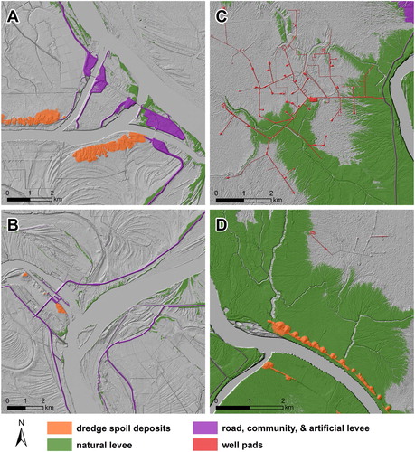
Figure 11. Annotated floodplain cross sections for the Old River AOI (profile A-A’) and Atchafalaya River AOI (profiles B-B’ and C-C’). The locations of the profiles are shown in Figure 4 (profile A-A’) and 6 (profiles B-B’ and C-C’). Arbitrary floodplain elevations (dashed horizontal grey lines) were selected to estimate volumes of different types of anthropogenic and natural features.

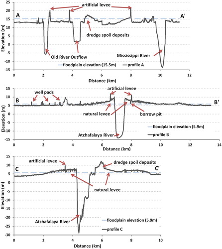
Slicing the topography of the Atchafalaya AOI at an arbitrary elevation of 5.9 masl – an elevation chosen to include the oil well pads – increases both the relative areas and volumes of natural levees (Figure 10(C,D)). However, the artificial levees, well pads, roads, spoil deposits, and other anthropogenic landforms comprise 19.7% of the volume above this elevation. A contrast of two cross profiles (Figures 6 and 11), B-B’ with artificial levees and the less confined C-C’, shows that the magnitude of positive dredged landforms here exceeds the elevations and dimensions of artificial levees. Being artificial, these features along the Atchafalaya are generally post-1900 (levees: 1908–1922; roads: dominantly early 1930s; dredge spoil: late 1930s; well pads: post-1940). These insights indicate that more research could be done to quantify rates and patterns of anthropogenic landform development compared to those landforms developed by natural hydrologic and geologic processes.

5.4. Geovisualization of rivers and the future

Merging of modern data sets using geovisualization mapping techniques increases the potential for geoscience education and communication (Mitasova et al., 2012). Geovisualization is an emerging area where artistic and cartographic choices help inform geoscientists and the public about large river floodplains and their alterations. For example, high spatial resolution data sets such as multi-beam echo-sounder with terrestrial 3D laser scanner data have been integrated to examine riverbank erosion during periods of flooding in the River Stoer, Germany (Nasermoaddeli & Pasche, 2008), while repeat 3D surveys can help us to easily delineate erosion/deposition process and their potential triggering factors (Longoni et al., 2016). Herein, we have demonstrated the coupling of data sets to examine 3D river terrain, and advocate its use across a much larger area in the altered alluvial rivers and floodplains of Louisiana.

6. Conclusion

Mapping and visualization of the alluvial landscapes of the lower Mississippi and Atchafalaya rivers in south Louisiana, USA, highlights many phenomena of interest. Both older data sets (i.e. Fisk’s (1944, 1952) maps) and more modern data (i.e. 3D high-resolution landscape views based on LiDAR) give different yet complementary types of information about these large alluvial rivers. Fisk’s maps informed scientists and the general public about the migration of the Mississippi River, and the related problems such as bank erosion, spatial variations in channel stability, and geological controls such as former oxbow lakes filled with fine sediments (termed ‘clay plugs’ by Fisk). Fisk may have given considerable thought to his choices of colours and patterns in his mapping, but never expressed these decisions in his reports. The newer data sets and technologies integrate data on river depths and land elevations, enable 2D and 3D visualizations, thus providing new insights. Examples include scour downstream of diversion structures, the differences in bed elevations of active and abandoned fluvial landforms, and the increased variety, extent and dimensions of anthropogenic landforms since Fisk’s initial mapping. We can also see how these landforms modify processes, such as increasing the sedimentation within artificial levees and excluding sedimentation outside. In addition, we now have the ability to view landscapes from different perspectives and angles, and are able to quantify areas and volumes of landforms using GIS.

The aesthetic and artistic appeal of the two different types of mapping is difficult to compare, but clearly both artists and scientists have found appeal in Fisk’s (1944) maps. Time will tell whether maps derived from combined hydrographic survey-land surface LiDAR data sets have similar artistic appeal, although many people do find them aesthetically attractive. Regardless, with the modern data sets, the addition of the 3D perspective gives insights that could drive new avenues of research into the changing nature of space and place in this vulnerable and greatly altered landscape.

Software

ESRI ArcMap, ArcScene, Online CityEngine Web Scenes, and Adobe Photoshop were used in this study.

Acknowledgements

Mohammad Almulla, formerly of the University of Florida and presently at Kuwait University, kindly shared the hydrographic data for this section of the Atchafalaya River. Reviewers John Lewin and Julian Ruddock, and Special Issue Guest Editor Stephen Tooth, gave helpful comments that strengthened the paper. Publication of this article was funded in part by the University of Florida Open Access Publishing Fund.

Disclosure statement

No potential conflict of interest was reported by the authors.

ORCID

Joann Mossa http://orcid.org/0000-0003-4192-6056

Yin-Hsuen Chen http://orcid.org/0000-0003-4809-5718

Chia-Yu Wu http://orcid.org/0000-0002-1884-1479

References

- Amoros, C., & Bornette, G. (2002). Connectivity and biocomplexity in waterbodies of riverine floodplains. Freshwater Biology, 47(4), 761–776. doi: 10.1046/j.1365-2427.2002.00905.x
- Bambach, C. C. (2003). Leonardo Da Vinci master draftsman. New York, NY: Metropolitan Museum of Art.
- Biland, J., & Çöltekin, A. (2017). An empirical assessment of the impact of the light direction on the relief inversion effect in shaded relief maps: NNW is better than NW. Cartography and Geographic Information Science, 44(4), 358–372. doi: 10.1080/15230406.2016.1185647
- Bratkova, M., Shirley, P., & Thompson, W. B. (2009). Artistic rendering of mountainous terrain. ACM Transactions on Graphics, 28(4), 1–17. doi: 10.1145/1559755.1559759
- Brown, A. G., Tooth, S., Chiverrell, R. C., Rose, J., Thomas, D. S. G., Wainwright, J., … Downs, P. (2013). The Anthropocene: Is there a geomorphological case? Earth Surface Processes and Landforms, 38(4), 431–434. doi: 10.1002/esp.3368
- Chen, Y.-H., Zick, S. E., & Benjamin, A. R. (2016). A comprehensive cartographic approach to evacuation map creation for Hurricane Ike in Galveston County, Texas. Cartography and Geographic Information Science, 43(1), 68–85. doi: 10.1080/15230406.2015.1014426
- Christophe, S., Duménieu, B., Turbet, J., Hoarau, C., Mellado, N., Ory, J., … Vanderhaeghe, D. (2016). Map style formalization: Rendering techniques extension for cartography. In Expressive 2016 the joint symposium on computational aesthetics and sketch-based interfaces and modeling and non-photorealistic animation and rendering (pp. 59–68). Lisbonne: The Eurographics Association.
- Coe, D. E. (2016). Revealing Washington’s hidden landforms with LiDAR. Olympia, WA: Washington State Joint Agency GIS Day.
- Cunningham, R., Gisclair, D., & Craig, J. (2003). The Louisiana statewide LiDAR project. Baton Rouge, LA.
- Durkin, P. R., Hubbard, S. M., Holbrook, J., & Boyd, R. (2018). Evolution of fluvial meander-belt deposits and implications for the completeness of the stratigraphic record. GSA Bulletin, 130(5–6), 721–739. doi: 10.1130/b31699.1
- ESRI. (2007). Geometrical interval. Retrieved from http://webhelp.esri.com/arcgisdesktop/9.2/index.cfm?topicname=geometrical_interval
- ESRI. (2017). Classifying numerical fields for graduated symbology. Retrieved from http://desktop.arcgis.com/en/arcmap/10.3/map/working-with-layers/classifying-numerical-fields-for-graduated-symbols.htm#
- Evans, I. S. (2012). Geomorphometry and landform mapping: What is a landform? Geomorphology, 137(1), 94–106. doi: 10.1016/j.geomorph.2010.09.029
- Fabrikant, S. I., Christophe, S., Papastefanou, G., & Maggi, S. (2012). Emotional response to map design aesthetics Giscience Conference. Columbus, OH.
- Fisk, H. N. (1944). Geological investigation of the alluvial valley of the lower Mississippi River. Washington, DC: US Army Corps of Engineers.
- Fisk, H. N. (1952). Geological investigation of the Atchafalaya basin and the problem of Mississippi River diversion. Vicksburg, MS.
- Gesch, D. B. (2009). Analysis of Lidar elevation data for improved identification and delineation of lands vulnerable to sea-level rise. Journal of Coastal Research, 10053, 49–58. doi: 10.2112/si53-006.1
- Imhof, E. (1982). Cartographic relief presentation. Berlin: de Gruyter.
- Jenks, G. F., & Caspall, F. C. (1971). Error on choroplethic maps: Definition, measurement, reduction. Annals of the Association of American Geographers, 61(2), 217–244. doi: 10.1111/j.1467-8306.1971.tb00779.x
- Johnson, J. M. (2001). Mapping ethnicity: Color use in depicting ethnic distribution. Cartographic Perspectives, 40, 12–31. Retrieved from http://cartographicperspectives.org/carto/index.php/journal/article/view/cp40-johnson
- Kennelly, P. J. (2008). Terrain maps displaying hill-shading with curvature. Geomorphology, 102(3), 567–577. doi: 10.1016/j.geomorph.2008.05.046
- Krinitzsky, E. L. (1996). The contributions of H.N. Fisk to engineering geology in the Lower Mississippi Valley. Engineering Geology, 45(1), 45–58. doi: 10.1016/S0013-7952(96)00006-3
- LeBlanc, R. J. (1996). Harold Norman Fisk as a consultant to the Mississippi River Commission, 1948–1964 — an eye-witness account. Engineering Geology, 45(1), 15–36. doi: 10.1016/S0013-7952(97)81955-2
- Lewin, J., Ashworth, P. J., & Strick, R. J. P. (2017). Spillage sedimentation on large river floodplains. Earth Surface Processes and Landforms, 42(2), 290–305. doi: 10.1002/esp.3996
- Longoni, L., Papini, M., Brambilla, D., Barazzetti, L., Roncoroni, F., Scaioni, M., & Ivanov, V. (2016). Monitoring riverbank erosion in mountain catchments using terrestrial laser scanning. Remote Sensing, 8(3), 241. doi: 10.3390/rs8030241
- Marston, B. E., & Jenny, B. (2015). Improving the representation of major landforms in analytical relief shading. International Journal of Geographical Information Science, 29(7), 1144–1165. doi: 10.1080/13658816.2015.1009911
- McPhee, J. (1989). The control of nature. New York, NY: Farrar, Straus and Giroux - Macmillan.
- Mitasova, H., Harmon, R. S., Weaver, K. J., Lyons, N. J., & Overton, M. F. (2012). Scientific visualization of landscapes and landforms. Geomorphology, 137(1), 122–137. doi: 10.1016/j.geomorph.2010.09.033
- Morris, C. (2015). Reckoning with “the Crookedest River in the world”: The maps of Harold Norman Fisk. The Southern Quarterly, 52(3), 30–44.
- Mossa, J. (2013). Historical changes of a major juncture: Lower Old River, Louisiana. Physical Geography, 34(4–5), 315–334. doi: 10.1080/02723646.2013.847314
- Mossa, J. (2016). The changing geomorphology of the Atchafalaya River, Louisiana: A historical perspective. Geomorphology, 252, 112–127. doi: 10.1016/j.geomorph.2015.08.018
- Mossa, J., Chen, Y.-H., Walls, S. P., Kondolf, G. M., & Wu, C.-Y. (2017). Anthropogenic landforms and sediments from dredging and disposing sand along the Apalachicola River and its floodplain. Geomorphology, 294, 119–134. doi: 10.1016/j.geomorph.2017.03.010
- Nasermoaddeli, M. H., & Pasche, E. (2008). Application of terrestrial 3D laser scanner in quantification of the riverbank erosion and deposition. In International conference on fluvial hydraulics. Izmir: Kubaba Congress Department and Travel Services. Retrieved from https://www.semanticscholar.org/paper/Application-of-terrestrial-3-D-laser-scanner-in-of-Nasermoaddeli-Pasche/ac7d0388e996dd750b5680d5840138592520b38a
- Paine, J., Andrews, J., Saylam, K., & Tremblay, T. (2015). Airborne LiDAR-based wetland and permafrost-feature mapping on an Arctic Coastal Plain, North Slope, Alaska. In Remote sensing of wetlands (pp. 413–434). Boca Raton, FL: CRC Press.
- Patterson, T. (2001). Dem manipulation and 3-D terrain visualization: Techniques used by the U.S. National Park Service. Cartographica: The International Journal for Geographic Information and Geovisualization, 38(1–2), 89–101. doi: 10.3138/8741-g618-5601-1125
- Patterson, T., & Jenny, B. (2011). The development and rationale of cross-blended hypsometric tints. Cartographic Perspectives, 69, 31–46. doi: 10.14714/CP69.20
- Pierik, H. J., Stouthamer, E., & Cohen, K. M. (2017). Natural levee evolution in the Rhine-Meuse Delta, the Netherlands, during the first millennium CE. Geomorphology, 295, 215–234. doi: 10.1016/j.geomorph.2017.07.003
- Rankin, W. (2017). Radical cartography. Retrieved from http://www.radicalcartography.net/index.html?fisk
- Rees, R. (1980). Historical links between cartography and art. Geographical Review, 70(1), 60–78. doi: 10.2307/214368
- Remo, J. W. F., Ryherd, J., Ruffner, C. M., & Therrell, M. D. (2018). Temporal and spatial patterns of sedimentation within the batture lands of the middle Mississippi River, USA. Geomorphology, 308, 129–141. doi: 10.1016/j.geomorph.2018.02.010
- Reuss, M. (2004). Designing the bayous: The control of water in the Atchafalaya basin, 1800–1995 (Vol. 3). College Station, TX: Texas A&M University Press.
- Richards, E. P. (Unknown). Louisiana geology. Retrieved from http://biotech.law.lsu.edu/climate/mississippi/fisk/fisk.htm
- Robinson, M. C. (1996). Harold N. Fisk: A luminescent man. Engineering Geology, 45(1), 37–44. doi: 10.1016/S0013-7952(96)00005-1
- Rowland, J. C., Dietrich, W. E., Day, G., & Parker, G. (2009). Formation and maintenance of single-thread tie channels entering floodplain lakes: Observations from three diverse river systems. Journal of Geophysical Research: Earth Surface, 114(F2), 1–19. doi: 10.1029/2008jf001073
- Rowland, J. C., Lepper, K., Dietrich, W. E., Wilson, C. J., & Sheldon, R. (2005). Tie channel sedimentation rates, oxbow formation age and channel migration rate from optically stimulated luminescence (OSL) analysis of floodplain deposits. Earth Surface Processes and Landforms, 30(9), 1161–1179. doi: 10.1002/esp.1268
- Saucier, R. T. (1996). A contemporary appraisal of some key Fiskian concepts with emphasis on Holocene meander belt formation and morphology. Engineering Geology, 45(1), 67–86. doi: 10.1016/S0013-7952(96)00008-7
- Slocum, T. A. (1999). Thematic cartography and geovisualization. Upper Saddle River, NJ: Pearson Prentice Hall.
- Smith, L. M. (1996). Fluvial geomorphic features of the Lower Mississippi alluvial valley. Engineering Geology, 45(1), 139–165. doi: 10.1016/S0013-7952(96)00011-7
- Smith, M. J., Goodchild, M. F., & Longley, P. A. (2015). Geospatial analysis, a comprehensive guide to principles, techniques and software tools (5th ed.). Winchelsea: The Winchelsea Press.
- Sofia, G., Fontana, G. D., & Tarolli, P. (2014). High-resolution topography and anthropogenic feature extraction: Testing geomorphometric parameters in floodplains. Hydrological Processes, 28(4), 2046–2061. doi: 10.1002/hyp.9727
- Szabó, J. (2010). Anthropogenic geomorphology: Subject and system. In J. Szabó, L. Dávid, & D. Lóczy (Eds.), Anthropogenic geomorphology: A guide to man-made landforms (pp. 3–10). Dordrecht: Springer Netherlands.
- U.S. Army Corps of Engineer New Orleans District. (2009). 2006 Atchafalaya River hydrographic survey book. Retrieved from http://www.mvn.usace.army.mil/Missions/Engineering/Geospatial-Section/ARHB_2006/
- U.S. Army Corps of Engineers New Orleans District. (Unpublished). 2007 Mississippi River hydrographic survey data. New Orleans, LA.