Geo-LiM: a new geo-lithological map for Central Europe (Germany, France, Switzerland, Austria, Slovenia, and Northern Italy) as a tool for the estimation of atmospheric CO₂ consumption

ABSTRACT

We present a new geo-lithological map for Central Europe (Geo-LiM). It was prepared taking into account the chemical and mineralogical composition of the outcropping rocks and paying attention in discriminating metamorphic rocks, that were classified according to the chemistry of protoliths. The map was used for estimating the atmospheric CO₂ consumed by the chemical weathering of silicates and carbonates. The map is made available in vector format [Donnini et al,. 2018. A new Geo-Lithological Map (Geo-LiM) for Central Europe (Germany, France, Switzerland, Austria, Slovenia, and Northern Italy) (Version 1.2) [Data set]. Zenodo Retrieved from https://zenodo.org/record/3530257], together with the computer code used to classify the lithologies and to join original maps. As a consequence, researchers can either replicate the product, or alter the code to derive a different lithological classification of the original geological maps, following the concept of Open Science.

KEYWORDS:

• Lithology
• Europe
• geology
• global carbon cycle
• chemical weathering
• computer code

1. Introduction

Carbon migrates among oceans, atmosphere, ecosystems, and geosphere and one million years is the threshold to define the ‘short-term’ and ‘long-term’ carbon cycles (e.g. Berner, 1991, 1994, 2004, 2006; Berner & Kothavala, 2001; Berner, Lasaga, & Garrels, 1983). The chemical weathering, that consume atmospheric CO₂ increasing river water alkalinity on ‘long-term’, represents the main sink of atmospheric CO₂ (e.g. Berner & Berner, 2012; Gaillardet, Dupré, Louvat, & Allegre, 1999; Garrels & Mackenzie, 1971; Mackenzie & Garrels, 1966; Meybeck, 1987; Probst, 1992; Tardy, 1986; Viers, Oliva, Dandurand, Dupré, & Gaillardet, 2007).

Starting from the relationship between alkalinity and runoff for different lithologies (Bluth & Kump, 1994; Hartmann, 2009; Hartmann, Jansen, Dürr, Kempe, & Köhler, 2009; Meybeck, 1986, 1987), the flux of atmospheric CO₂ consumed by chemical weathering for a given area can be estimated knowing the runoff and the lithology. This approach does not consider the portion of carbon that returns to the atmosphere in the ‘long-term’, and for this reason, it is applicable only on ‘short-term’ (Amiotte-Suchet & Probst, 1993a; Amiotte-Suchet & Probst, 1993b; Amiotte-Suchet & Probst, 1995; Amiotte-Suchet, Probst, & Ludwig, 2003; Hartmann, 2009; Hartmann et al., 2009; Probst, Mortatti, & Tardy, 1994).

In this paper we introduce a geo-lithological map for Central Europe (Germany, France, Switzerland, Austria, Slovenia, and Northern Italy) at 1:1,000,000 scale with lithological classification compliant to the methods most used in literature for estimating the consumption of atmospheric CO₂ by chemical weathering. The map, named Geo-LiM, is downloadable in vector format (https://zenodo.org/record/3530257; Donnini, Marchesini, & Zucchini, 2018) together with the computer code used to classify the lithologies and to join the original maps.

Finally, we show a comparison of the atmospheric CO₂ consumed by chemical weathering using Geo-LiM and GLiM (Hartmann & Moosdorf, 2012) that is the more recent global lithological map available from the literature.

2. Theoretical background

The knowledge of the chemical and mineralogical composition of the rocks outcropping in river basins is essential for estimating the atmospheric CO₂ consumed by chemical weathering. Different lithological maps, at the global scale, exist, and some of them are schematized in Table 1.

Table 1. Global lithological maps available from the literature.

Name	Scale/Resolution	Lithologies	Digital format	Ref.
	2° × 2°	(i) carbonates, (ii) shales, (iii) sandstones, (iv) extrusive igneous rocks, (v) shield areas (intrusive igneous rocks and metamorphic rocks), and (vi) ‘complicated lithology’	Raster	Gibbs and Kump (1994)
	1° × 1°	(i) sands and sandstone, (ii) shales, (iii) carbonate rocks, (iv) shield rocks (intrusive igneous rocks and metamorphic rocks), (v) acid volcanic rocks, and (vi) basalts	Raster	Amiotte-Suchet et al. (2003)
	1:25,000,000	(i) acid volcanic rocks, (ii) basic volcanic rocks, (iii) acid plutonic rocks, (iv) basic plutonic rocks, (v) Precambrian basement, (vi) metamorphic rocks, (vii) consolidated siliciclastic rocks, (viii) mixed sedimentary rocks, (ix) carbonates, (x) semi- to un-consolidated sedimentary rocks, (xi) alluvial deposits, (xii) loess, (xiii) dunes, (xiv) evaporites, and (xv) complex lithology (sediments, volcanic and metamorphic rocks)	Vector	Dürr et al. (2005)
GLiM	1:1,000,000	(i) evaporites, (ii) metamorphics, (iii) acid plutonic rocks, (iv) basic plutonic rocks, (v) intermediate plutonic rocks, (vi) pyroclastics, (vii) carbonate sedimentary rocks, (viii) mixed sedimentary rocks, (ix) siliciclastic sedimentary rocks, (x) unconsolidated sediments, (xi) acid volcanic rocks, (xii) basic volcanic rocks, (xiii) intermediate volcanic rocks, (xiv) precambrian rocks, and (xv) complex lithologies	Vector	Hartmann and Moosdorf (2012)

None of the maps reported in Table 1 fully discriminate metamorphic rocks according to the chemistry of protoliths, which is relevant to perform the analysis of the atmospheric CO₂ consumption. At regional scale (Alpine region), the lithological map published by Donnini et al. (2016) try to lithologically classify, wherever possible, metamorphic rocks according to the chemistry of protoliths. Only a small portion of the original metamorphic rocks are unclassified. The map was published at 1:1,000,000 nominal scale and considers 8 lithologies: (i) acid igneous rocks, (ii) mixed carbonate, (iii) clay and claystone, (iv) debris, (v) mafic rocks, (vi) unclassified metamorphic rocks, (vii) pure carbonate rocks, and (viii) sandstone.

3. Study area

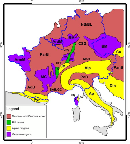
The study area includes the European territory of Germany, France, Switzerland, Austria, Slovenia, and Northern Italy. The European continent is the result of the convergence of the European and African continental plates that caused the closure of an ancient ocean located in the Mediterranean zone. The oceanic crust was then subducted causing the collision of continental blocks that formed the current European mountain ranges. The Figure 1 depicts the main physiographic/tectonic provinces of Central Europe (Crampon, Custodio, & Downing, 1996; Marroni & Pandolfi, 2003; Müller et al., 1992; Neubauer, 2009; Pfiffner, 2014) and the abbreviations are explained in the caption of the figure. A number of collisions between continents have occurred during the evolution of European continent and, accordingly to their ages, we distinguish between Caledonian (Early Paleozoic), Variscan (also named Hercynian, Late Paleozoic) and Alpine (from Jurassic to Cretaceous) orogenies. In the study area, the last two orogens outcrop. The Variscan mountain chains have an ‘island-like’ distribution, that is the results of the erosion of a continuous mountain range covered with younger sediments (Mesozoic and Cenozoic cover in Figure 1), while the Alpine orogens have often an arc and winding shape due to the geometry of the plate boundaries (Pfiffner, 2014).

Figure 1. Tectonic scheme of Central Europe. Mesozoic and Cenozoic cover: AqB = Aquitanian Basin, ParB = Paris Basin, UEF = Uplands of Eastern France, NS/BL = North Sea and Baltic Lowlands, CSG = Central and Southern Germany, MoB = Molasse Basin, PanB = Pannonian Basin, PoB = Po Basin, SAB/GC = Sub Alpine Basin and Grands Causses; Rift basins: LG = Limagne Graben, URG = Upper Rhine Graben; Alpine orogens: AC = Alpine Corsica, Pyr = Pyrenees, JM = Jura Mountains, Alp = Alps, Ap = Apennines, Din = Dinarides, Ca = Carpathians; Variscan orogens: HC: Hercynian Corsica, MC = Massif Central, ArmM = Armorican Massif, VM = Vosges Mountains, BF = Black Forest, ArdM = Ardenne Mountains, RM = Resnish Massif, BM = Bohemian Massif. (Modified from Crampon et al., 1996; Marroni & Pandolfi, 2003; Müller et al., 1992; Neubauer, 2009; Pfiffner, 2014). In blue the Geo-LiM study area is shown. In grey are shown the regions outside from our study area.

4. Materials and methods

Geo-LiM was elaborated in vector format at 1:1,000,000 scale starting from the geological information derived from the vector maps reported in Table 2.

Table 2. National geological maps used to elaborate Geo-LiM.

Nation	Scale	Field containing geological information	Language	Ref.
Italy	1:500,000	‘DESCR’	Italian	http://www.isprambiente.gov.it
Switzerland	1:500,000	‘LITH_PET’, ‘LITHO’, ‘LEG_GEOL’	French	http://www.swisstopo.admin.ch
Germany	1:100,000	‘EN_PETROG’, ‘EN_PET’, ‘URN_LITH_1’, ‘URN_LITH_2’, ‘URN_LITH_3’, ‘URN_LITH_4’, ‘URN_LITH_5’	English	BGR, 2011
Austria	1:500,000	‘LEGTEXT_EN’, ‘LITHOL_EN’	English	http://www.geologie.ac.at
France	1:1,000,000	‘urn_litho1’, ‘urn_litho2’, ‘urn_litho3’, ‘urn_litho4’, ‘urn_litho5’	English	http://www.europe-geology.eu/metadata
Slovenia	1:250,000	‘urn_litho1’, ‘urn_litho2’, ‘urn_litho3’, ‘urn_litho4’, ‘urn_litho5’	English	http://www.europe-geology.eu/metadata

The six maps have different coordinate reference systems and different accuracy and information quality. Several topological errors (e.g. gaps between polygon borders, overlapping polygon borders, etc …) were observed in France, Germany and Slovenia geological maps and were corrected removing duplicate boundaries and the longest boundary with adjacent areas (smaller than, respectively, 1, 600 and 50 m²).

Starting from the geological information available in the attribute tables of the 6 geological maps, we performed a lithological classification of the vector polygons, applying complex set of SQL (Structured Query Language) instructions listed in Donnini et al., 2018 (https://zenodo.org/record/3530257). Classification was accurate and particular attention was paid not to create lithological contacts across the boundaries of different countries.

The lithological classification of the vector polygons was performed by expert judgment based on the geological information available in the attribute columns of the original geological maps. These kinds of procedure, widely adopted in the literature ( Amiotte-Suchet et al., 2003 ; Donnini et al., 2016 ; Dürr, Meybeck, & Dürr, 2005 ; Gibbs & Kump, 1994 ; Hartmann & Moosdorf, 2012 ), is different from the one used for geochemical mapping that requires (i) chemical/isotopic analyses of samples collected in the field and (ii) geo-informatic interpolation tools (e.g. Chiprés, Salinas, Castro-Larragoitia, & Monroy, 2008; Fiannacca et al., 2017; McKinley, 2013; Morris, Pirajno, & Shevchenko, 2003; Ortolano, Cirrincione, Pezzino, Tripodi, & Zappalà, 2015; Reimann et al., 1998; Smith, Cannon, Woodruff, Solano, & Ellefsen, 2014).

In the following the ten lithologies of Geo-LiM are described.

‘Pure carbonate’ includes rocks composed mainly of calcite, aragonite, and dolomite such as limestone, dolomite, and travertine, as well as marble (Boggs Jr & Boggs, 2009; Garrels & Mackenzie, 1971; Pettijohn, 1957).

‘Mixed carbonate’ includes calcarenites and marls, rocks composed of carbonate minerals mixed up with non-carbonate minerals (Pettijohn, 1957).

‘Gypsum evaporite’ included gypsum and anhydrite.

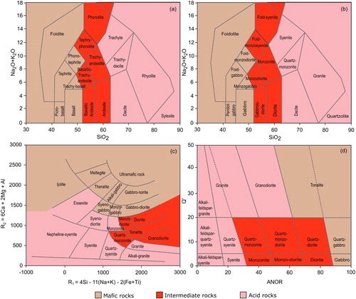
The subdivision among ‘acid rocks’, ‘mafic rocks’, and ‘intermediate rocks’ was done according to (i) the TAS (Total-Alkali-Silica) diagram (Bas, Maitre, Streckeisen, & Zanettin, 1986; Middlemost, 1994) (see Figure 2a), (ii) its adaptation for plutonic rocks (Bas et al., 1986; Middlemost, 1994) (see Figure 2b), (iii) the R₁-R₂ diagram (De La Roche, Leterriere, Grandclaude, & Marchal, 1980) (see Figure 2c), and (iv) the Q′-ANOR diagram (Streckeisen & Le Maitre, 1979) (see Figure 2d). These four plots are among the most used geochemical classification diagrams for discriminating igneous rocks (e.g. Fiannacca et al., 2017).

Figure 2. Chemical classification and nomenclature of (a) volcanic rocks and (b) plutonic rocks using the total alkali versus silica (TAS) diagram (modified from Middlemost, 1994), (c) R₁-R₂ diagram (modified from De La Roche et al., 1980) and (d) Q’-ANOR diagram (modified from Streckeisen & Le Maitre, 1979) for plutonic rocks. Q’=Q × 100/(Q + Ab + Or + An); ANOR = (100 × An/(An + Or). Q: quartz, Ab: albite, Or: orthoclase, An: anorthite.

The metamorphic rocks, with either an acid or mafic protoliths, were classified according to Mottana, Crespi, and Liborio (2009). For this reason, an orthogneiss was considered as ‘acid rocks’ (assuming a granitic protolith composition), and a serpentinite was considered as ‘mafic rocks’.

‘Sandstones’ category includes arkose, greywacke (Garrels & Mackenzie, 1971), and conglomerate that, as highlighted by Boggs Jr and Boggs (2009), is similar to sandstone in terms of origin and depositional mechanisms. The metamorphic rock quartzite was considered as ‘sandstones’, considering its protholite (Mottana et al., 2009).

‘Claystones’ category includes shale, argillite, siltstone and mudstone (Boggs Jr & Boggs, 2009; Garrels & Mackenzie, 1971). Considering their protoliths, the metamorphic rocks phyllite, schists and paragneiss were considered as ‘claystones’ (Mottana et al., 2009).

According to Garrels and Mackenzie (1971) and to Herron (1988), sandstone and claystone could contain a non-negligible carbonate component. Garrels and Mackenzie (1971) show that the weight percentage of normative mineral composition of some average sandstone and claystone coming from literature are always under 5%, while Herron (1988), using additional samples, shows that these lithologies could have a major carbonate component. In detail, Herron (1988), subdivided the terrigenous sands and shales in ‘noncalcareous’ (Ca > 4%), ‘calcareous’ (4% < Ca < 15%) and ‘carbonate’ (Ca > 15%). However, in the present work no analytical data on the geochemical composition of the classified lithologies were used. Thus, geological polygons containing arenaceous and argillaceous rocks, were respectively classified in the ‘sandstones’ and in the ‘claystones’ categories, when carbonate rocks presence was not explicitly reported.

The generic ‘metamorphic rocks’ category was used only when information on protoliths were unavailable or unclear (e.g. in the case of migmatite, mylonite, and metasediments).

The last category considered was ‘peat’.

Some problems arose to classify rocks composed by more than one lithotypes.

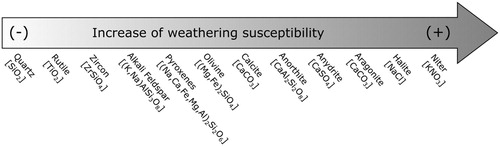
Considering the weathering series of both silicate and non-silicate minerals (Railsback, 2006) (Figure 3), the rocks composed by a mix of carbonate and gypsum/anhydrite were included in the ‘gypsum evaporite’ category, and the rocks composed by more than one lithotypes where at least one of them is composed by ‘mixed carbonate rocks’ were included in the ‘mixed carbonate rocks’ category (it is the case of a lithotype composed by sandstone, greywacke and marl that was included in the ‘mixed carbonate rocks’ category).

Figure 3. Weathering series of silicates (Goldich, 1938) modified adding some non-silicates minerals (Railsback, 2006). The simplified general mineral formulas are reported. (The figure is modified from Railsback, 2006)

In the case of silicate rocks composed by more than one lithotypes, the ‘principle of prevalence’ was adopted, classifying these rocks according to the most abundant lithologies reported in the attribute tables. For example, as the attribute table of a polygon reported the presence of basalt, trachy-basalt and andesite, we classified that polygon as ‘basic rocks’ since both basalt and trachy-basalt were considered ‘basic rocks’, whereas only andesite is within the class ‘intermediate rocks’.

5. Geo-LiM: the new Geo-Lithological Map of Central Europe

5.1. Comments to the map

Figure 4 shows Geo-LiM map, downloadable in vector format (GPKG) and in printable A0 format (PDF) (https://zenodo.org/record/3530257; Donnini et al., 2018). In the attribute table we provide also a column (named LithologyValue) containing the classification of the lithologies according to the LithologyValue dictionary defined by the INSPIRE Data Specification on Geology (http://inspire.ec.europa.eu/codelist/LithologyValue).

Figure 4. The Geo-LiM map. The colors used to distinguish the different lithologies were derived from the lithologic legend adopted by the United States Geological Survey (USGS) for the geologic maps of US states and made available by USGS together with the RGB codes in the web (https://mrdata.usgs.gov/catalog/lithclass-color.php).

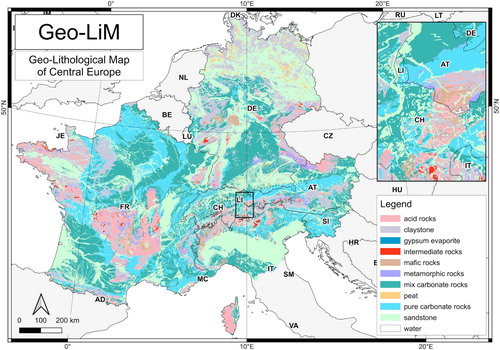
Here follows a brief description of Geo-LiM where the abbreviations are the same used in section §3. An overview of the map confirms the presence of the Hercynian basement constituted by igneous rocks (both effusive and plutonic) and metamorphic rocks (Crampon et al., 1996) in the Variscan orogens (MC, ArmM, VM, BF, ArdM, RM, HC, and BM) highlighted in Geo-LiM by ‘acid rocks’ and secondly by ‘intermediate rocks’ and ‘mafic rocks’ (for the codes used in this sub-session, see Figure 1).

Regarding the Alpine orogens, the map highlights the prevalence of ‘pure carbonate rocks’ in the JM (Arnaud-Vanneau & Arnaud, 1990) and in the Din (Velić, 2007). Ophiolites (‘mafic rocks’) and turbiditic materials (‘mixed carbonate rocks’) are shown in the northern sector of Ap (Molli et al., 2010) and in AC (Carmignani, Conti, Cornamusini, & Meccheri, 2004; Marroni & Pandolfi, 2003). The map confirms an inner crystalline core constituted by ‘acid rocks’, ‘mafic rocks’ and ‘intermediate rocks’ north- and south-bounded by ‘pure carbonate rocks’ and ‘mixed carbonate rocks’ in the Alp (Crampon et al., 1996; Donnini et al., 2016; Rossi & Donnini, 2018). Finally, in Pyr the map shows crystalline rocks (Crampon et al., 1996) in the form of ‘acid rocks’, ‘mafic rocks’ and ‘claystone’; whereas, in the western sector of Ca, the map shows flishoid deposits (Janoschek & Matura, 1980) as ‘mixed carbonate rocks’.

LG and URG rift basins, as well as the Mesozoic and Cenozoic covers (AqB, ParB, UEF, NS/BL, CSG, MoB, PanB, PoB, and SAB/GC), are mainly constituted by ‘sandstone’ (Crampon et al., 1996).

In Table 3 the abundance of outcropping rock types calculated in the area of Geo-LiM (∼1,170,000 km²) is shown. Carbonate rocks are the most abundant lithology with a total of 40.77% subdivided in 26.73% of ‘mixed carbonate’ and 14.04% of ‘pure carbonate’. It follows ‘sandstone’ (30.57%), ‘claystone’ (15.55%) and volcanic rocks (with 7.93% of ‘acid rocks’, 1.65% of ‘mafic rocks’, and 0.39% of ‘intermediate rocks, for a total of 9.97%). ‘Metamorphic rocks’, ‘peats’ and ‘gypsum evaporite’ represent less than 2% of the study area (respectively 1.42%, 1.18% and 0.02%). A small area (0.52%) is covered by water in the form of lakes and glaciers.

Table 3. Relative abundance (% Area), mean and standard deviation (sd) of elevation, expressed in meters above the sea level (m. asl), and slope, expressed in degrees (°), of outcropping rocks in the Geo-LiM area.

Rock type	% Area	Elevation (m. asl)		Slope (°)
		mean	sd	mean	sd
Sandstone	30.57	246.6	329.4	3.7	5.9
Mixed carbonate	26.73	441.1	457.7	7.5	8.6
Claystone	15.55	449.5	621.6	7.3	9.8
Pure carbonate	14.04	572.1	581.1	10.5	11.8
Acid rocks	7.93	735.3	645.7	10.9	10.9
Mafic rocks	1.65	889.9	693.8	12.2	11.4
Metamorphic rocks	1.42	807.3	638.0	10.9	10.8
Peat	1.18	90.2	169.1	1.1	1.4
Water (lakes and glaciers)	0.52	1448.4	1330.6	10.7	14.1
Intermediate rocks	0.39	649.3	736.3	10.1	11.2
Gypsum evaporite	0.02	437.3	506.3	10.0	7.6

Moreover, the Table 3 shows the elevation and slope calculated for each lithology starting from the 25 m resolution EUDEM (https://www.eea.europa.eu/data-and-maps/data/copernicus-land-monitoring-service-eu-dem).

The results highlight that ‘water’ category (lakes and glaciers) has high mean elevation and slope values (1448.4 m and 10.7°) associated with high standard deviations (1330.6 m and 14.1°). This is because in ‘water’ we included lakes (usually located in valleys) and glaciers (at high altitude). It follows the igneous and metamorphic rock types ‘mafic rocks’, ‘metamorphic rocks’, ‘acid rocks’, and ‘intermediate rocks’ with quite high mean elevation (from 889.9 m. to 649.3 m.) and slope values (from 12.2° 10.1°) and quite high standard deviation values. These lithologies are associated to the mountains of the Variscan orogens MC, ArmM, VM, BF, ArdM, RM, HC, and BM, as well as to the crystalline core of the Alpine chain.

Medium elevation (from 572.1 m. to 437.3 m.) and slope (from 10.5° to 7.3°) values are shown for ‘pure carbonate, ‘claystone’, ‘mixed carbonate’, and ‘gypsum evaporite’ associated to the northern AC, Din, western Ca, JM and to the calcareous mountains of the northern and southern bounds of the Alpine chain.

‘Sandstone’, abundant in the LG and URG rift basins and in the Mesozoic/Cenozoic covers (AqB, ParB, UEF, NS/BL, CSG, MoB, PanB, PoB, SAB/GC), presents low mean elevation (246.6 m.) and slope values (3.7°).

The lowest mean elevation (90.2 m.) and slope values (31.1°) is shown for ‘peat’, formed by the degradation of the vegetation in flattened wetlands (Bracco, 2004).

In general, the standard deviations of the slope and elevation are similar or of the same order of magnitude with respect to the mean values, reflecting the high heterogeneity of those variables in the spatial domains of the different lithologies.

5.2. Comparison with the global lithological map GLiM

Geo-LiM was compared with the more recent global lithological map available from the literature, that is GLiM (Hartmann & Moosdorf, 2012). Table 4 shows the relative abundance (in terms of area percentage) of outcropping rocks of GLiM in the study area of Geo-LiM. Table 4 shows that, in the GLiM, 70.38% of the study area is constituted by carbonate sedimentary rocks (‘sc’), unconsolidated sediments (‘su’), and mixed sedimentary rocks (‘sm’). Similar values are shown for Geo-LiM (see Table 2), where the sum of ‘sandstone’, ‘mixed carbonate’, ‘claystone’ and ‘pure carbonate’ represents 86.88% of the study area. The percentages of igneous rocks are similar for the two maps (7.94% in GLiM and 9.97% in Geo-LiM). Differences exist in the percentages of metamorphic rocks that represent 11.01% in Hartmann and Moosdorf (2012) and 1.42% in Geo-LiM, demonstrating the attention paid in elaborating Geo-LiM to discriminate metamorphic rocks, classified according to the chemistry of protoliths.

Table 4. Relative abundance (% Area) of outcropping rocks from the global lithological map GLiM (Hartmann & Moosdorf, 2012) in the study (Geo-LiM) area. Code and descriptions are from Hartmann and Moosdorf (2012).

Code	Description	% Area
sc	carbonate sedimentary rocks	27.16
su	unconsolidated sediments	24.51
sm	mixed sedimentary rocks	18.71
mt	metamorphics	11.01
ss	siliciclastic sedimentary rocks	10.08
pa	acid plutonic rocks	5.38
vb	basic volcanic rocks	1.24
va	acid volcanic rocks	0.82
wb	water bodies	0.48
pb	basic plutonic rocks	0.41
ig	ice and glaciers	0.07
pi	intermediate plutonic rocks	0.06
nd	no data	0.03
py	pyroclastics	0.02
vi	intermediate volcanic rocks	0.01
ev	evaporites	0.00

We overlaid the map here presented (Geo-LiM) with the global lithological map GLiM to quantify the differences between the two maps, even considering the spatial matching of the lithological classification. The results are shown in Figure 5 where the colored bars represent the 11 lithologies of Geo-LiM, the short codes indicate the GLiM lithological classes (Hartmann & Moosdorf, 2012) reported in Table 4, the oblique lines pattern represents the percentage of areas where the two maps do not match in terms of lithologies, and the cross lines pattern represents the percentage of areas where the differences among lithology classifications do not allow for a direct comparison.

Figure 5. Results of the overlay among Geo-LiM and the global lithological map GLiM (Hartmann & Moosdorf, 2012). The coloured bars represent the 11 lithologies of Geo-LiM. The short codes indicate the GLiM lithological classes (Hartmann & Moosdorf, 2012): mt = metamorphics, sc = carbonate sedimentary rocks, sm = mixed sedimentary rocks, su = unconsolidated sediments, ss = siliciclastic sedimentary rocks, va = acid volcanic rocks, pa = acid plutonic rocks, pb = basic plutonic rocks, pa = acid plutonic rocks, ig = ice and glaciers, wb = water bodies.

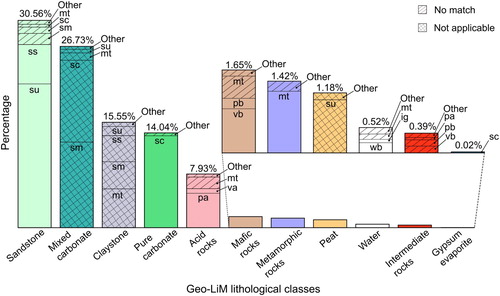
The figure shows a very good match for the Geo-LiM classes ‘pure carbonate’, and ‘metamorphic rocks’ (97.08% and 85.92%, respectively, of territory of those classes having the same classification in both Geo-LiM and GLiM maps). The same can be said for the ‘sandstone’, assuming that the corresponding classes of GLiM are the unconsolidated sediments (‘su’) and the siliciclastic sedimentary rocks (‘ss’). A good match is also observed for ‘acid rocks’ and ‘mafic rocks’ (respectively 73.74% and 65.85%), when considering that the GLiM ‘mt’ class (that represents respectively 22.47% and 26.83% of the Geo-LiM acid and mafic rocks) is discriminated, in Geo-LiM, considering the chemistry of metamorphic protholits (see section §3). Worst matches are shown (i) for ‘water’, where the lithologies in the two maps, depending on the scale of the maps, could represent the rocks that host rivers and glaciers, (ii) for ‘intermediate rocks’, probably due to different methods adopted by Hartmann & Moosdorf, 2012 to discriminate that kind of rocks. However, ‘water’ and ‘intermediate rocks’ represent less than 1% (0.39% and 0.52%) of the studied area. The less represented lithology in the Geo-LiM map, the ‘gypsum evaporite’, i.e. a hydrated calcium sulphate (CaSO₄·2H₂O), is wrongly associated to ‘sc’ (carbonate sedimentary rocks) in GLiM, lithology that outcrops only in 0.02% of the study area.

Notwithstanding some of the Geo-LiM lithologies do not find a clear counterpart in the GLiM classification, the result of the overlay highlights that there is a general concordance among the classification of the two maps. In particular: (i) ‘mixed carbonate’ category is coherently subdivided mainly in ‘sm’ (mixed sedimentary rocks, 47.38%) and ‘sc’ (carbonate sedimentary rocks, 45.29%); (ii) ‘claystone’ is coherently subdivided mainly in ‘mt’ (metamorphic, 36.96%), ‘sm’ (mixed sedimentary rocks, 25.95%), ‘ss’ (siliciclastic sedimentary rocks, 25.02%) and ‘su’ (unconsolidated sediments rocks, 8.89%). Finally, (iii) ‘peat’, that does not exist in GLiM, matches mainly with ‘su’ (unconsolidated sediments, 88.24%), coherently with the materials that compose the flattened wetlands. In general, the percentage of match between the lithologies of Geo-LiM and GLiM is equal to 83.19% excluding the GLiM metamorphic rocks (‘mt’), while it rises up to 92.85% when ‘mt’ is considered a protolith of the Geo-LiM classes. As a consequence, 16.81% and 7.15% represent, respectively, the percentages of the non-matching lithologies between the two maps when either we do not consider or we include the ‘mt’ class.

In general, we observed a strong general concordance among the two maps. Furthermore, the Geo-LiM map improved the discrimination of the metamorphic rocks, based on the analysis of the protolites. Close to 90% of the GLiM metamorphic rocks (corresponding to 9.59% of the study area extent) are assigned, in Geo-LiM, to another lithological class.

6. Atmospheric CO₂ consumption in Central Europe

The flux of atmospheric CO₂ consumed by chemical weathering (ΦCO₂ ) for Central Europe was estimated using the empirical relationships that link, for different lithologies, ΦCO₂ to the runoff (RO) (Amiotte-Suchet et al., 2003; Amiotte-Suchet & Probst, 1993a; Amiotte-Suchet & Probst, 1993b; Amiotte-Suchet & Probst, 1995; Bluth & Kump, 1994; Hartmann, 2009; Hartmann et al., 2009; Probst et al., 1994). Table 5 shows the angular coefficients (m) of these relationships for the six lithologies considered by Amiotte-Suchet et al. (2003) and estimated considering more than 200 French mono-lithological river basins (Meybeck, 1986; Meybeck, 1987). Table 4 also represents a lookup table between those coefficients and the Geo-LiM and GLiM (Hartmann & Moosdorf, 2012) lithologies.

Table 5. Angular coefficient (m) of the relationships between the flux of atmospheric CO₂ consumed by chemical weathering and the runoff estimated by Amiotte-Suchet et al., 2003 for the six lithologies considered by the authors. In the table also the corresponding lithologies considering Geo-LiM (this work) and GLiM (Hartmann & Moosdorf, 2012) are shown.

Rock category			m [mol l^−1]
1° × 1° Global lithological map (Amiotte-Suchet et al., 2003)	Geo-LiM	GLiM (Hartmann & Moosdorf, 2012)	(Amiotte-Suchet et al., 2003)
Carbonate rocks	Mixed carbonate, pure carbonate, gypsum evaporite, peat	Carbonate sedimentary rocks, mixed sedimentary rocks, evaporites, complex lithologies	1.59 × 10^−3
Shales	Claystone		6.27 × 10^−4
Basalts	Mafic rocks	Basic plutonic rocks, basic volcanic rocks	4.79 × 10^−4
Acid volcanic rocks	Acid rocks	Acid plutonic rocks, acid volcanic rocks, pyroclastics	2.22 × 10^−4
Sands and sandstone	Sandstone	Siliciclastic sedimentary rocks, unconsolidated sediments	1.52 × 10^−4
Shield rocks	Metamorphic rocks, intermediate rocks	Metamorphics, intermediate plutonic rocks, intermediate volcanic rocks, precambrian rocks	9.50 × 10^−5

For the study area, two ΦCO₂ maps, Figure 6a and Figure 6b, at 1 km × 1 km resolution were elaborated considering respectively Geo-LiM and GLiM (Hartmann & Moosdorf, 2012) by applying equation Equation (1)(1) $\mathrm{\Phi }C{O}_2=m\times RO$(1) where m values were derived from Table 5, and RO values were derived from a 1 km × 1 km mean monthly RO map (Figure 6d) here elaborated by using the 1950–2015 monthly RO rates (Gudmundsson & Seneviratne, 2016).

Figure 6: (a) ΦCO₂ map elaborated using Geo-LiM; (b) ΦCO₂ map elaborated using GLiM (Hartmann & Moosdorf, 2012); (c) difference between Figure 6a and Figure 6b; (d) 1 km × 1 km mean monthly runoff (RO) map elaborated using the 1950 - 2015 monthly RO rates of E-RUN version 1.1 (Gudmundsson & Seneviratne, 2016).

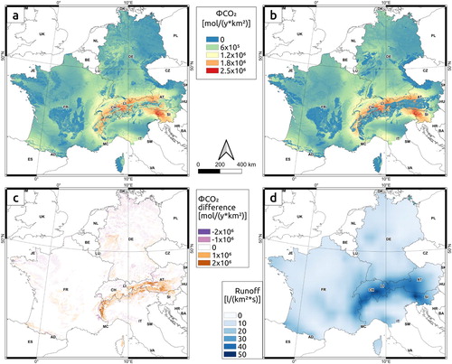
The ΦCO₂ rates estimated considering Geo-LiM and GLiM, respectively 4.93 × 10⁵ mol y⁻¹ km⁻² and 4.78 × 10⁵ mol y⁻¹ km⁻², differ of about 3% each other and are of the same order of magnitude of the world average values available from the literature (e.g 2.46 × 10⁵ mol y⁻¹ km⁻² from Gaillardet et al., 1999 and 2.59 × 10⁵ mol y⁻¹ km⁻² form Amiotte-Suchet et al., 2003). This confirms the quality of the two maps elaborated following independent approaches.

Locally, some differences exist between the two ΦCO₂ maps (Figure 6a and Figure 6b), as highlighted by Figure 6c, that shows the differences between the two maps, and by Table 6, that shows the differences between ΦCO₂ rates estimated considering Geo-LiM and GLiM within each GLiM lithological class (Hartmann & Moosdorf, 2012). The table highlights that the highest differences per unit area (expressed in mol y⁻¹ km⁻²) are observed for: pyroclastic rocks (‘py’: 9.13 × 10⁵ mol y⁻¹ km⁻²), metamorphic rocks (‘mt’: 3.57 × 10⁵ mol y⁻¹ km⁻²), no data (‘nd’: 2.17 × 10⁵ mol y⁻¹ km⁻²) and water bodies (‘wb’: 2.01 × 10⁵ mol y⁻¹ km⁻²). Looking at the ΦCO₂ produced by each single lithology (expressed in mol y⁻¹) in the whole area, the highest differences are observed for mixed sedimentary rocks (‘sm’: −1.67 × 10¹⁰ mol y⁻¹) and for metamorphic rocks (‘mt’: 4.66 × 10¹⁰ mol y⁻¹). The negative value for ‘sm’ means that for the areas occupied by this lithology, associated to ‘carbonate rocks’ of Amiotte-Suchet et al. (2003), GLiM (Hartmann & Moosdorf, 2012) is more prone to consume atmospheric CO₂. This is because ‘sm’ category is composed by ‘all sediments where carbonate is mentioned but not dominant, plus some units that were identified as sediments, but no information on the type of sediment was available’ (Hartmann & Moosdorf, 2012) that in Geo-LiM are splitted within ‘mixed carbonate’ and ‘claystone’ categories (see Figure 5), the first one more prone to consume atmospheric CO₂ than the second one (see Table 5). Conversely, the positive value for ‘mt’ (associated to the lithology less prone to consume atmospheric CO₂, see Table 5) in Geo-LiM is splitted in rock categories more prone to consume CO₂ (see Figure 5).

Table 6. Differences between ΦCO₂ rates estimated considering Geo-LiM and GLiM (ΦCO₂ difference) within each GLiM lithological class (Hartmann & Moosdorf, 2012) expressed in [mol y⁻¹ km⁻²] and in [mol y⁻¹]. Code and description are from Hartmann and Moosdorf (2012). Lithologies are ordered from the most to the least abundant.

Code	Description	ΦCO2 difference [(ΦCO2)Geo-LiM - (ΦCO2)GLiM] [mol y^−1 km^−2 ]	ΦCO2 difference [(ΦCO2)Geo-LiM - (ΦCO2)GLiM] [mol y^−1 ]
sc	carbonate sedimentary rocks	−1.90 × 10^4	−6.10 × 10^9
su	unconsolidated sediments	−1.60 × 10^3	−5.18 × 10^8
sm	mixed sedimentary rocks	−7.60 × 10^4	−1.67 × 10^10
mt	metamorphics	3.57 × 10^5	4.66 × 10^10
ss	siliciclastic sedimentary rocks	−6.23 × 10^4	−7.76 × 10^9
pa	acid plutonic rocks	6.18 × 10^3	3.92 × 10^8
vb	basic volcanic rocks	2.16 × 10^3	3.10 × 10^7
va	acid volcanic rocks	5.64 × 10^4	5.38 × 10^8
wb	water bodies	2.01 × 10^5	1.27 × 10^9
pb	basic plutonic rocks	1.43 × 10^4	6.88 × 10^7
ig	ice and glaciers	8.57 × 10^2	6.77 × 10^5
pi	intermediate plutonic rocks	9.56 × 10^4	6.96 × 10^7
nd	no data	2.17 × 10^5	7.62 × 10^7
py	pyroclastics	9.13 × 10^5	2.85 × 10^8
vi	intermediate volcanic rocks	8.89 × 10^4	7.29 × 10^6

Figure 6c shows that the highest differences between the two ΦCO₂ maps are located in the Alps, that is an area (i) particularly affected by metamorphism (see e.g. Ernst, 1973) and (2) characterized by high RO values (Figure 6d).

Considering the entire study area, the total amount of ΦCO₂ estimated yearly using Geo-LiM and GLiM (Hartmann & Moosdorf, 2012) is 5.78 × 10¹¹ mol y⁻¹ and 5.59 × 10¹¹ mol y⁻¹, respectively. These values represent a small percentage, between 2% and 3%, of the ΦCO₂ estimated at global scale by different authors: 2.4 × 10¹³ mol y⁻¹ by Gaillardet et al. (1999), 2.13 × 10¹³ mol y⁻¹ by Amiotte-Suchet et al. (2003), 1.84 × 10¹³ mol y⁻¹ by Munhoven (2002), and 1.98 × 10¹³ mol y⁻¹ by Hartmann et al. (2009). The comparison of these values with the atmospheric CO₂ released by anthropic activity, estimated to be equal to 4.42 × 10¹⁴ mol y⁻¹ by Prentice et al. (2001), highlights the impact of human activity on the natural processes involved in the global carbon cycle.

7. Conclusions

In this paper we presented a new geo-lithological map of Central Europe (Germany, France, Switzerland, Austria, Slovenia, and Northern Italy) at 1:1,000,000 scale named Geo-LiM.

Differently to the global lithological maps available in the literature (Gibbs & Kump, 1994; Amiotte-Suchet et al., 2003; Dürr et al., 2005; Hartmann & Moosdorf, 2012), a big effort was made to discriminate metamorphic rocks that were classified according to the chemistry of protoliths, including in the class ‘metamorphic rocks’ only the rocks for which data on protoliths were unavailable or unclear. Following this methodology, in the study area the ‘metamorphic rocks’ class represents only 1.42%, versus the 11.01% value calculated in the same area considering the more recent global lithological map GLiM of Hartmann and Moosdorf (2012). However, the comparison performed between Geo-LiM and GLiM demonstrated a general good correlation between the two maps.

Finally, the two maps (Geo-LiM and GLiM), together with runoff values derived by Gudmundsson and Seneviratne (2016), were used to estimate the atmospheric CO₂ consumed by chemical weathering. The results are very similar and of the same order of magnitude of the world average values available from the literature (e.g Gaillardet et al., 1999 and Amiotte-Suchet et al., 2003), confirming the quality of the two maps elaborated following independent approaches. Looking in detail, some local differences exist, in particular in the Alps where metamorphic rocks are abundant (see e.g. Ernst, 1973).

Since lithology is a fundamental variable in various scientific fields as, for example, geomorphology, hydrogeology, and geochemistry, we think that Geo-LiM and the possible different classifications that can be obtained using the computer code provided along with the map (https://zenodo.org/record/3530257; Donnini et al., 2018), is a reason of novelty. Following the concept of Open Science (Nüst et al., 2018), it is allowed the reproducibility of the product and the alteration of the code to derive a different lithological classification of the original geological maps, accordingly to different applications. The lithological classification was performed based on expert judgment and, as a consequence, can be considered accurate but also very subjective. For this reason we made available the queries adopted for the classification, in order to allow the verification, the reproducibility and, possibly, the modification of the classification procedure.

Software

The pre-processing (cleaning of topological errors) and processing (unions, intersections and classifications) procedures necessary to elaborate the map were performed using GRASS GIS (Neteler & Mitasova, 2008; Neteler, Bowman, Landa, & Metz, 2012), an open source GIS software, and PostgreSQL (http://www.postgresql.org), an open source relational database management system (RDBMS), with its PostGIS spatial extension (http://www.postgis.org). The layout used for creating the A0 map was produced using QGIS (https://www.qgis.org), an open source desktop GIS software.

Data

The Geo-Lithological Map of Central Europe (Geo-LIM: Donnini et al., 2018) was released in GPKG and in PDF format at the following web address: https://zenodo.org/record/3530257, together with (i) the original national geological maps of Germany, Italy, Slovenia, France, Switzerland and Austria, used for creating the map; (ii) the procedures used to classify and to combine the maps that can be used to replicate the product.

Acknowledgements

M. Donnini was supported by a grant of the Fondazione Assicurazioni Generali, and A. Zucchini was partially supported by the research projects of Paola Comodi, Francesco Frondini and Diego Perugini of the Department of Physics and Geology of the University of Perugia.

M. Donnini ideates and coordinates the work, paying attention on the accuracy of the final map with the geology of Central Europe; I. Marchesini mainly contributed to the geographical and statistical operations; and A. Zucchini mainly contributed to the mineralogical-petrographic considerations useful for elaborating the geo-lithological classification of the map. M. Donnini wrote the paper that I. Marchesini and A. Zucchini revised internally.

Disclosure statement

No potential conflict of interest was reported by the authors.

Additional information

Funding

This work was supported by Università degli Studi di Perugia: [Grant Number Partially supported by the research projects of Pa]; Fondazione Generali: [Grant Number Grant].

References

- Amiotte-Suchet, P. A. , & Probst, J. L. (1995). A global model for present-day atmospheric/soil CO2 consumption by chemical erosion of continental rocks (GEM-CO2). Tellus B: Chemical and Physical Meteorology , 47 (1-2), 273–280. doi: 10.3402/tellusb.v47i1-2.16047
- Amiotte-Suchet, P. , & Probst, J. L. (1993a). Flux de CO2 consommé par altération chimique continentale: Influences du drainage et de la lithologie = CO2 flux consumed by chemical weathering of continents: Influences of drainage and lithology. Comptes-rendus de L'Académie des Sciences de Paris-Série II, Mécanique, physique, chimie, astronomie , 317 , 615–622.
- Amiotte-Suchet, P. , & Probst, J. L. (1993b). Modelling of atmospheric CO2 consumption by chemical weathering of rocks: Application to the Garonne, Congo and Amazon basins. Chemical Geology , 107 (3-4), 205–210. doi: 10.1016/0009-2541(93)90174-H
- Amiotte-Suchet, P. , Probst, J. L. , & Ludwig, W. (2003). Worldwide distribution of continental rock lithology: Implications for the atmospheric/soil CO2 uptake by continental weathering and alkalinity river transport to the oceans. Global Biogeochemical Cycles , 17 (2). doi: 10.1029/2002GB001891
- Arnaud-Vanneau, A. , & Arnaud, H. (1990). Hauterivian to Lower Aptian carbonate shelf sedimentation and sequence stratigraphy in the Jura and northern Subalpine chains (southeastern France and Swiss Jura). Spec. Publs int. Ass. Sediment , 9 , 203–233.
- Bas, M. L. , Maitre, R. L. , Streckeisen, A. , Zanettin, B. , & IUGS Subcommission on the Systematics of Igneous Rocks . (1986). A chemical classification of volcanic rocks based on the total alkali-silica diagram. Journal of Petrology , 27 (3), 745–750. doi: 10.1093/petrology/27.3.745
- Berner, E. K. , & Berner, R. A. (2012). Global environment: Water, air, and geochemical cycles . Princeton: Princeton University Press.
- Berner, R. A. (1991). A model for atmospheric CO2 over phanerozoic time. American Journal of Science;(United States) , 291 (4), 339–376.
- Berner, R. A. (1994). GEOCARB II: A revised model of atmospheric CO2 over phanerozoic time. American Journal of Science;(United States) , 294 (1), 182–204.
- Berner, R. A. (2004). The Phanerozoic carbon cycle: CO2 and O2 . Oxford: Oxford University Press on Demand.
- Berner, R. A. (2006). Inclusion of the weathering of volcanic rocks in the GEOCARBSULF model. American Journal of Science , 306 (5), 295–302. doi: 10.2475/05.2006.01
- Berner, R. A. , & Kothavala, Z. (2001). GEOCARB III: A revised model of atmospheric CO2 over Phanerozoic time. American Journal of Science , 301 (2), 182–204. doi: 10.2475/ajs.301.2.182
- Berner, R. A. , Lasaga, A. C. , & Garrels, R. M. (1983). The carbonate-silicate geochemical cycle and its effect on atmospheric carbon dioxide over the past 100 million years. American Journal of Science , 283 , 641–683. doi: 10.2475/ajs.283.7.641
- BGR . (2011). Geologische Karte der Bundesrepublik Deutschland 1:1,000,000 (GK1000) . Hannover : BGR.
- Bluth, G. J. , & Kump, L. R. (1994). Lithologic and climatologic controls of river chemistry. Geochimica et Cosmochimica Acta , 58 (10), 2341–2359. doi: 10.1016/0016-7037(94)90015-9
- Boggs Jr, S. , & Boggs, S. (2009). Petrology of sedimentary rocks . Cambridge: Cambridge University Press.
- Bracco, F. (2004). Mountain peat bogs: Relicts of biodiversity in acid waters (Vol. 9) . Udine: Museo friulano di storia naturale.
- Carmignani, L. , Conti, P. , Cornamusini, G. , & Meccheri, M. (2004). The internal Northern Apennines, the northern Tyrrhenian sea and the Sardinia-Corsica block. Geology of Italy. Special Volume, Italian Geological Society, IGC , 32 , 59–77.
- Chiprés, J. A. , Salinas, J. C. , Castro-Larragoitia, J. , & Monroy, M. G. (2008). Geochemical mapping of major and trace elements in soils from the Altiplano Potosino, Mexico: A multiscale comparison. Geochemistry: Exploration, Environment, Analysis , 8 , 279–290. doi: 10.1144/1467-7873/08-181
- Crampon, N. , Custodio, E. , & Downing, R. A. (1996). The hydrogeology of Western Europe: A basic framework. Quarterly Journal of Engineering Geology and Hydrogeology , 29 (2), 163–180. doi: 10.1144/GSL.QJEGH.1996.029.P2.05
- De La Roche, H. , Leterriere, J. , Grandclaude, P. , & Marchal, M. (1980). A classification of volcanic and plutonic rocks using R1, R2-diagrams and major elements analysis-its relationship with current nomenclature. Chemical Geology , 29 , 183–210. doi: 10.1016/0009-2541(80)90020-0
- Donnini, M. , Frondini, F. , Probst, J. L. , Probst, A. , Cardellini, C. , Marchesini, I. , & Guzzetti, F. (2016). Chemical weathering and consumption of atmospheric carbon dioxide in the Alpine region. Global and Planetary Change , 136 , 65–81. doi: 10.1016/j.gloplacha.2015.10.017
- Donnini, M. , Marchesini, I. , & Zucchini, A. (2018). A new Geo-Lithological Map (Geo-LiM) for Central Europe (Germany, France, Switzerland, Austria, Slovenia, and Northern Italy) (Version 1.0) [Data set]. Zenodo. https://zenodo.org/record/3530257
- Dürr, H. H. , Meybeck, M. , & Dürr, S. H. (2005). Lithologic composition of the Earth’s continental surfaces derived from a new digital map emphasizing riverine material transfer. Global Biogeochemical Cycles , 19 (4), 1–22.
- Ernst, W. G. (1973). Interpretative synthesis of metamorphism in the Alps. Geological Society of America Bulletin , 84 (6), 2053–2078. doi:10.1130/0016-7606(1973)84<2053:ISOMIT>2.0.CO;2
- Fiannacca, P. , Ortolano, G. , Pagano, M. , Visalli, R. , Cirrincione, R. , & Zappalà, L. (2017). IG-Mapper: A new ArcGIS® toolbox for the geostatistics-based automated geochemical mapping of igneous rocks. Chemical Geology , 470 , 75–92. doi: 10.1016/j.chemgeo.2017.08.024
- Gaillardet, J. , Dupré, B. , Louvat, P. , & Allegre, C. J. (1999). Global silicate weathering and CO2 consumption rates deduced from the chemistry of large rivers. Chemical Geology , 159 (1-4), 3–30. doi: 10.1016/S0009-2541(99)00031-5
- Garrels, R. M. , & Mackenzie, F. T. (1971). Evolution of sedimentary rocks . New York : Norton.
- Gibbs, M. T. , & Kump, L. R. (1994). Global chemical erosion during the last glacial maximum and the present: Sensitivity to changes in lithology and hydrology. Paleoceanography , 9 (4), 529–543. doi: 10.1029/94PA01009
- Goldich, S. S. (1938). A study in rock-weathering. The Journal of Geology , 46 (1), 17–58. doi: 10.1086/624619
- Gudmundsson, L. , & Seneviratne, S. I. (2016). Observation-based gridded runoff estimates for Europe (E-RUN version 1.1). Earth System Science Data , 8 (2), 279–295. doi: 10.5194/essd-8-279-2016
- Hartmann, J. (2009). Bicarbonate-fluxes and CO2-consumption by chemical weathering on the Japanese Archipelago—application of a multi-lithological model framework. Chemical Geology , 265 (3-4), 237–271. doi: 10.1016/j.chemgeo.2009.03.024
- Hartmann, J. , Jansen, N. , Dürr, H. H. , Kempe, S. , & Köhler, P. (2009). Global CO2-consumption by chemical weathering: What is the contribution of highly active weathering regions? Global and Planetary Change , 69 (4), 185–194. doi: 10.1016/j.gloplacha.2009.07.007
- Hartmann, J. , & Moosdorf, N. (2012). The new global lithological map database GLiM: A representation of rock properties at the Earth surface. Geochemistry, Geophysics, Geosystems , 13 , 1–37. doi: 10.1029/2012GC004370
- Herron, M. M. (1988). Geochemical classification of terrigenous sands and shales from core or log data. Journal of Sedimentary Research , 58 (5), 820–829.
- Janoschek, W. , & Matura, A. (1980). Outline of the geology of Austria . Wien: Geologische Bundesanstalt.
- Mackenzie, F. T. , & Garrels, R. M. (1966). Chemical mass balance between rivers and oceans. American Journal of Science , 264 (7), 507–525. doi: 10.2475/ajs.264.7.507
- Marroni, M. , & Pandolfi, L. (2003). Deformation history of the ophiolite sequence from the Balagne Nappe, northern Corsica: Insights in the tectonic evolution of Alpine Corsica. Geological Journal , 38 (1), 67–83. doi: 10.1002/gj.933
- McKinley, J. M. (2013). How useful are databases in environmental and criminal forensics? Geological Society, London, Special Publications , 384 , 109–119. doi: 10.1144/SP384.9
- Meybeck, M. (1986). Composition chimique des ruisseaux non pollués en France. Chemical composition of headwater streams in France. Sciences Géologiques. Bulletin , 39 (1), 3–77. doi: 10.3406/sgeol.1986.1719
- Meybeck, M. (1987). Global chemical weathering of surficial rocks estimated from river dissolved loads. American Journal of Science , 287 (5), 401–428. doi: 10.2475/ajs.287.5.401
- Middlemost, E. A. (1994). Naming materials in the magma/igneous rock system. Earth-Science Reviews , 37 (3-4), 215–224. doi: 10.1016/0012-8252(94)90029-9
- Molli, G. , Crispini, L. , Malusà, M. , Mosca, P. , Piana, F. , & Federico, L. (2010). Geology of the Western Alps-Northern Apennine junction area: A regional review. Journal of the Virtual Explorer , 36 , 1–49. doi: 10.3809/jvirtex.2010.00215
- Morris, P. A. , Pirajno, F. , & Shevchenko, S. (2003). Proterozoic mineralization identified by integrated regional regolith geochemistry, geophysics and bedrock mapping in Western Australia. Geochemistry: Exploration, Environment, Analysis , 3 (1), 13–28. doi: 10.1144/1467-787302-041
- Mottana, A. , Crespi, R. , & Liborio, G. (2009). Minerali e rocce . Milano: Illustrati Mondadori.
- Munhoven, G. (2002). Glacial–interglacial changes of continental weathering: Estimates of the related CO2 and HCO3− flux variations and their uncertainties. Global and Planetary Change, 33(1-2), 155-176. doi: 10.1016/S0921-8181(02)00068-1
- Müller, B. , Zoback, M. L. , Fuchs, K. , Mastin, L. , Gregersen, S. , Pavoni, N. , … Ljunggren, C. (1992). Regional patterns of tectonic stress in Europe. Journal of Geophysical Research , 97 (B8), 11783–11803. doi: 10.1029/91JB01096
- Neteler, M. , Bowman, M. H. , Landa, M. , & Metz, M. (2012). GRASS GIS: A multi-purpose open source GIS. Environmental Modelling and Software , 31 , 124–130. doi: 10.1016/j.envsoft.2011.11.014
- Neteler, M. , & Mitasova, H. (2008). Open source GIS: A GRASS GIS approach. Third edition The International series in Engineering and computer Science vol. 773 . New York : Springer. (406 pp.).
- Neubauer, F. (2009). Geology of Europe. In B. De Vivo , B. Grasemann , & K. Stüwe (Eds.), GEOLOGY-Volume V . Oxford : EOLSS Publications.
- Nüst, D. , Granell, C. , Hofer, B. , Konkol, M. , Ostermann, F. O. , Sileryte, R. , & Cerutti, V. (2018). Reproducible research and GIScience: An evaluation using AGILE conference papers. PeerJ , 6 , e5072. doi: 10.7717/peerj.5072
- Ortolano, G. , Cirrincione, R. , Pezzino, A. , Tripodi, V. , & Zappalà, L. (2015). Petro-structural geology of the Eastern Aspromonte Massif crystalline basement (southern Italy- Calabria): an example of interoperable geo-data management from thin section- to field scale. Journal of Maps , 11 (1), 181–200. doi: 10.1080/17445647.2014.948939
- Pettijohn, F. J. (1957). Sedimentary rocks (Vol. 2) . New York : Harper and Brothers.
- Pfiffner, O. A. (2014). Geology of the Alps . Oxford: John Wiley and Sons.
- Prentice, I. C. , Farquhar, G. D. , Fasham, M. J. R. , Goulden, M. L. , Heimann, M. , Jaramillo, V. J. , … Wallace, D. W. (2001). The carbon cycle and atmospheric carbon dioxide . Cambridge: Cambridge University Press.
- Probst, J. L. (1992). Géochimie et hydrologie de l'érosion continentale. Mécanismes, bilan global actuel et fluctuations au cours des 500 derniers millions d'années (Vol. 94, No. 1) . Strasbourg: Persée-Portail des revues scientifiques en SHS.
- Probst, J. L. , Mortatti, J. , & Tardy, Y. (1994). Carbon river fluxes and weathering CO2 consumption in the Congo and Amazon River basins. Applied Geochemistry , 9 (1), 1–13. doi: 10.1016/0883-2927(94)90047-7
- Railsback, L. B. (2006). Some fundamentals of mineralogy and geochemistry. On-line book, quoted from: www.gly.uga.edu/railsback
- Reimann, C. , Äyräs, M. , Cheklushin, V. , Bogatyrev, I. , Boyd, R. , De Caritat, P. , … Volden, T. (1998). Environmental Geochemical Atlas of the Central Barents Region. NGU-GTK-CKE Special Publication (82-7385- 176-1, Geol. Surv. of Nor., Trondheim, Norway).
- Rossi, M. , & Donnini, M. (2018). Estimation of regional scale effective infiltration using an open source hydrogeological balance model and free/open data. Environmental Modelling & Software , 104 , 153–170. doi: 10.1016/j.envsoft.2018.03.005
- Smith, D. B. , Cannon, W. F. , Woodruff, L. G. , Solano, F. , & Ellefsen, K. J. (2014). Geochemical and mineralogical maps for soils of the conterminous United States. U.S. Geological Survey Open-File Report , 1082 , 386. doi: 10.3133/ofr20141082
- Streckeisen, A. L. , & Le Maitre, R. W. (1979). A chemical approximation to the modal QAPF classification of the igneous rock. Neues Jb. Mineral. Abh , 136 , 169–206.
- Tardy, Y. (1986). Le cycle de l'eau: climats, paléoclimats et géochimie globale . Paris: Masson.
- Velić, I. (2007). Stratigraphy and Palaeobiogeography of Mesozoic Benthic Foraminifera of the Karst Dinarides (SE Europe)-PART 1. Geologia Croatica , 64 (1), 1–16. doi: 10.4154/gc.2011.01
- Viers, J. , Oliva, P. , Dandurand, J. L. , Dupré, B. , & Gaillardet, J. (2007). Chemical weathering rates, CO2 consumption, and control parameters deduced from the chemical composition of rivers. In J. I. Drever (Ed.), Surface and Ground water, weathering, and Soils. Treatise on geochemistry, Volume 5 (pp. 1–25). Oxford: Elsevier. Executive Editors: H.D. Holland and K.K. Turekian.
- Web sites
- https://zenodo.org/record/3530257
- http://www.isprambiente.gov.it
- http://www.swisstopo.admin.ch
- http://www.geologie.ac.at
- http://www.europe-geology.eu/metadata
- https://mrdata.usgs.gov/catalog/lithclass-color.php
- https://www.eea.europa.eu/data-and-maps/data/copernicus-land-monitoring-service-eu-dem
- http://www.postgresql.org
- http://www.postgis.org
- https://www.qgis.org