Interactive display of surnames distributions in historic and contemporary Great Britain

ABSTRACT

We introduce a method to calculate and store approximately 1.2 million surname distributions calculated for surnames found in Great Britain for six years of historic population data and 20 years of contemporary population registers compiled from various consumer sources. We subsequently show how this database can be incorporated into an interactive web-environment specifically designed for the public dissemination of detailed surname statistics. Additionally, we argue that the database can be used in the quantitative analysis of surnames in Great Britain and potentially offer valuable insights into processes of contagious and hierarchical diffusion of populations as well as the regional distinctiveness of demographic change and stasis.

KEYWORDS:

• Interactive visualisation
• web mapping
• surname geographies
• kernel density estimation

1. Introduction

When it comes to hereditary surnames or family names, two important observations can be made. First, in many countries, including the United Kingdom, surnames are vertically transmitted through the patrilineal line from generation to generation (Jobling, 2001). Secondly, as a result of varying socio-spatial differences in naming practices, surnames can be traced back to a national or regional origin (Cheshire, 2014; Cheshire et al., 2010; Cheshire & Longley, 2012). Because of these properties, together with their relatively high level of availability, surnames have been used in a variety of studies, ranging from inferring ethnicity (Lan et al., 2018; Mateos et al., 2011) to identifying probable genetically close individuals for sampling purposes (Kandt et al., 2016). Similarly, surname analysis has been used to estimate the likely origins of migrants (Bloothooft & Darlu, 2013; Degioanni & Darlu, 2001) and more recently to uncover processes of demographic change and stasis (Kandt et al., 2020).

So far, however, relatively little is done to disseminate surname research to a wider audience, with only University College London’s, now outdated, Worldnames and Great Britain’s names online databases being notable exceptions. In what follows, we first introduce a method that effectively stores approximately 1.2 million unique surname distributions estimated for historic and contemporary Great Britain. We subsequently show how this database can be incorporated into a contemporary web-environment, how we can interactively map the calculated surname distributions, and how consumer statistics can be linked to the calculated surname distributions to create individual surname profiles. Lastly, we argue that the database can be used for further research, and can potentially offer valuable insights into processes of contagious and hierarchical diffusion of populations as well as the regional distinctiveness of demographic change and stasis (see also Van Dijk et al., 2019; Van Dijk & Longley, 2020).

2. Data sources

Historic Censuses provide a valuable source of information on the population of Great Britain and its change over time. Individual-level records are made publicly available following 100 years after their collection date. Higgs and Schürer (2014) have brought together and standardised digital transcriptions of most of the censuses of Great Britain for the period 1851–1911 with the Integrated Census Microdata Project (I-CeM). Besides standardised birthplace strings and occupational titles (see Schürer et al., 2015), the full census microdata also contains full addresses. Unfortunately, geocoding these historic address-level data using contemporary street-network data is, albeit very promising, work in progress (see Lan & Longley, 2019). However, fortunately, addresses are also linked to parishes, the boundaries of which have been digitised in two sets of consistent parish geographies.

Because contemporary censuses do not disclose names and addresses, extensive databases of surnames at the addresses-level of enfranchised adults were sought from public versions of the electoral register from 1997 until 2016, with supplements from consumer data from 2002 onwards to capture those that opt-out or are not eligible to vote. However, these ‘Consumer Registers’ do not have full coverage of the adult population and are of unknown provenance. To bolster their coverage, the data are linked and ‘hardened’ through processes of fuzzy address matching and cross-referencing counts with Office for National Statistics’ Mid-Year population estimates. Because of these processes of internal and external validation, the Consumer Registers are found to be largely representative of the majority of the UK’s adult population (see Lansley et al., 2018, 2019).

3. Estimating, storing, and retrieving surname distributions of large data sets

3.1. Kernel density estimation

One way to analyse and compare individual surname distributions over time without being hindered by changing administrative areas is by point pattern analysis. We first assign every individual found in the historic census data to the centroid of the parish with which they are associated. Similarly, we geocode all individuals found in the Consumer Registers directly through the coordinates associated with each postcode. We subsequently describe the spatial patterns of the population-weighted point events on a year-by-year and surname-by-surname basis through a process called Kernel Density Estimation (KDE). KDE is a non-parametric method that places a search window (kernel) over a point and uses the information within this kernel to estimate point densities and has a variety of applications, for instance, in school catchment area analysis (Singleton et al., 2011), health research (Carlos et al., 2010), as well as surname research (Cheshire & Longley, 2012).

A KDE applied over two-dimensional space can be formally described as follows (Shi, 2010, p. 643):(1) $\hat{f}\left(x,y\right)=\frac{1}{n{h}^2}\sum _{i=i}^{n}K\left(\frac{d_{i,\left(x,y\right)}}{h}\right)$(1) where $\hat{f}\left(x,y\right)$ is the estimated density at location $\left(x,y\right)$, n is the number of point events that fall within the bandwidth h, $d_{i,\left(x,y\right)}$ is the distance between the location $\left(x,y\right)$ and an event point i. Lastly, K is the density function that describes the contribution of point i to the estimated density at location $\left(x,y\right)$. The outcome is a ‘smooth, continuous surface where each location in the study area is assigned a density value irrespective of arbitrary administrative boundaries’ (Carlos et al., 2010, p. 1).

For each surname, the isotropic fixed bandwidth is estimated using a likelihood cross-validation method, constrained by a minimum bandwidth of 5 kilometres and a maximum bandwidth of 40 kilometres. For computational reasons, we estimate the bandwidth on a sample of the surname population in cases where a surname has more than 5000 bearers. Although it is theoretically possible to vary the bandwidth according to the distribution of the background data to accommodate local variations, this is extremely challenging for large data sets (cf. Zhang et al., 2017). For the historic data, KDEs are only calculated for surnames that have at least 30 bearers, while for the contemporary Consumer Registers the surname populations must consist of at least 50 individuals. All KDE calculations are executed using the R programming language (R Core Team, 2018) using the ‘Sparr’ package (Davies et al., 2018).

3.2. Parallel processing

A major challenge of the KDE approach is its processing time. KDEs are relatively slow to compute, and we, therefore, cannot generate them ‘on the fly’ for interactive display. As such, all kernel density calculations need to be executed and subsequently stored. Given the large number of surnames, this means we would benefit from parallel processing techniques. At the same time, however, because arguably all individual KDEs to be processed can be considered as a collection of data sets of ‘medium’ size (Soundararaj et al., 2019), we do not need complicated and large distributed clusters for our calculations. As such, to speed up processing times, all calculations are parallelised using GNU Parallel (Tange, 2011) and distributed over a high-performance Linux cluster consisting of eight computing nodes (Intel Xeon E5-2630 v3 processor; 32 cores, 2.4 GHz; 128GB memory). By utilising the Unix shell pipe to connect multiple processes, a list of available surnames can be fed to GNU Parallel. In turn, the programme parallelises the sequence of retrieving our input data from a PostgreSQL database (using psql), sending the retrieved data to the R KDE script, and finally pushing R’s output to our PostgreSQL database (using psql). The total number of calculated KDEs for each year, the number of individuals that are represented by these KDEs, and the size of the entire population that is available in our data set is shown in Table 1 and Table 2 for the Historic Censuses and the Consumer Registers, respectively.

Table 1. Number of calculated KDEs for the Historic Censuses.

Year	Extent	Surnames (n > = 30)	Individuals KDE (surname n)	Historic Census (total n)
1851	England, Scotland, Wales	37,941	18,947,318	20,610,325
1861	England, Scotland, Wales	48,894	20,468,217	22,837,378
1881	England, Scotland, Wales	39,845	28,051,183	29,865,602
1891	England, Scotland, Wales	50,097	31,038,153	33,522,822
1901	England, Scotland, Wales	44,807	35,226,626	36,910,767
1911	England, Wales	44,961	33,817,546	36,353,455

Table 2. Number of calculated KDEs for the consumer registers.

Year	Source	Surnames (n > = 50)	Individuals KDE (surname n)	Consumer Register (total n)
1997	Electoral register	41,221	42,079,244	45,128,535
1998	Electoral register	42,271	43,823,946	46,982,475
1999	Electoral register	42,600	44,200,014	47,383,720
2000	Electoral register	42,602	44,017,002	47,224,708
2001	Electoral register	42,030	42,904,961	46,111,068
2002	Consumer sources	43,094	43,967,574	47,284,306
2003	Consumer sources	42,944	42,969,604	46,326,823
2004	Consumer sources	43,363	43,066,049	46,574,935
2005	Consumer sources	43,684	42,591,771	46,247,329
2006	Consumer sources	44,366	42,745,564	46,614,786
2007	Consumer sources	45,301	43,220,899	47,300,978
2008	Consumer sources	46,042	43,550,015	47,798,322
2009	Consumer sources	47,275	44,788,305	49,269,002
2010	Consumer sources	48,692	45,943,563	50,687,293
2011	Consumer sources	48,324	45,251,279	50,135,397
2012	Consumer sources	48,721	44,503,643	49,835,696
2013	Consumer sources	49,737	45,452,932	51,266,951
2014	Consumer sources	50,335	45,843,928	52,247,265
2015	Consumer sources	50,196	45,416,064	52,614,295
2016	Consumer sources	50,404	45,298,145	53,520,333

3.3. Grid deconstruction

Because we deal with over a million surname geographies, not only processing speed is an issue; we also require an efficient way of storing these data. Ideally, all the surname geographies are stored in full, to avoid information loss. However, a disadvantage of employing KDEs to describe surname distributions is that KDEs are calculated over a grid and also outputted as such; in case of the United Kingdom, a rectangular grid for the entire country with a resolution of 1 square kilometre results in over 870,000 grid cells. For over one million surname distributions this has a significant impact on the size of the final database, with exponentially more storage required with an increase in grid resolution. A conservative estimate is that for every 100,000 surnames around 400GB of storage is required when unique grids are stored in full.

A possible solution is to extract contours (isolines) from the raster and vectorise these contours. A major drawback of this method is that it is an expensive procedure in terms of processing time. Another potential solution would be to decrease the grid resolution, however, this results per definition in information loss. Arguably a more viable angle is to look into the data and the structure of the data itself. Because the resulting KDEs for a large share of surnames result in empty grid cells, the grid essentially becomes a sparse matrix. As such, we do not have to consider all the entries but rather focus on the location and values of all the non-empty entries of this sparse matrix. We then can use the concept of a sparse matrix to minimise the space required for storing all our surname geographies.

Whilst some packages in the R programming language allow for efficient in-memory manipulation of sparse matrices, for example ‘Matrix’ (Bates & Maechler, 2018), the data output is returned in the Harwell Boeing sparse matrix file format which is not ideal for storage in an object-relational database. Similarly, PostgreDynamic, a modified version of the ‘standard’ object-relational PostgreSQL data model, can efficiently store sparse matrices but only on a table by table basis (Corwin et al., 2007). This is not suitable for our current purpose either as this would result in the creation of more than a million individual tables. Also, more recent solutions for dealing with raster data in an online environment, such as Cloud Optimised GeoTIFFs, cannot be exploited. These solutions rather focus on the setting up raster files in such a way that it is possible to serve parts the parts of the file that are requested by a client, e.g. a certain geographic area, through ‘streaming’ the required tiles instead of loading the entire raster file.

Given our challenging storage requirements and the unsuitability of available methods, we develop a method to compress the raster information by turning to some of the strategies deployed in sparse matrix compression. Two well-known strategies to compress spare matrices are: (1) to store the raster in separate one-dimensional arrays that contain only contain the non-zero values and the locations of these non-zero values within the raster, sometimes known as the ‘Yale sparse matrix format’, or (2) to create a dictionary of keys that maps all unique values to all row, column pairs. The first method is optimised for efficient access and common matrix operations and the second method is more efficient when it comes to quickly modifying the data. We are not interested in matrix operations, nor are we interested in modifying the data after the calculations, so both methods are suitable. For simplicity reasons, we choose to adopt the first method.

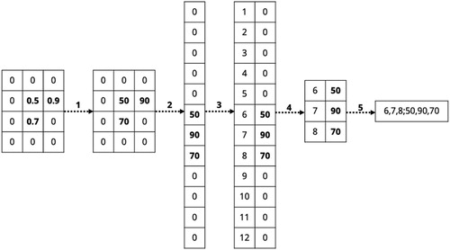
All our analyses are applied onto the same geographical area, Great Britain, and this means that for every surname that is processed the output grid is consistent in resolution, extent, and shape. This means we only have to store the XY-coordinates of the output grid once. We first flatten the matrix into one dimension and store every XY-coordinate together with their index position within the flattened matrix. For each surname distribution, we then extract the point density estimates for each cell in a similar fashion. We start by rescaling all the density estimates on a scale ranging from 0 to 100 to make the results of different years and surname distributions comparable with one another. We then flatten the matrix and for every index position, we subsequently retain the point density estimate. Hereafter we apply our sparse matrix compression: only index, value pairs are retained if the value is non-zero. Finally, we write the resulting data frame to an ordered string as a concatenation of all indexes and all values that can be stored in a PostgreSQL database. Figure 1 graphically summarises this process of matrix (1) standardising, (2) flattening, (3) indexing, (4) compressing, and (5) converting the index, value pairs to its string representation.

Figure. 1 Raster grid deconstruction.

3.4. Grid reconstruction

Whether it is for online interactive visualisation or analysis purposes, the stored deconstructed grids need to be dynamically reconstructed. This can easily be done using the ‘Pandas’ Python library through performing an inner join on the stored index, value pairs with the XY-coordinates of the grid using index value as a key (McKinney, 2010). In many cases, however, we are only interested in part of the data such as the area with the highest relative density. Similarly, the raster requires some transformation to make it informative to a wider audience. We do this by transforming the portions of the raster with the highest relative densities into vector polygons that can be displayed in an online environment.

Transforming selected raster points into vector polygons is not trivial. We start by selecting the points we are interested in; in this example scaled kernel density estimates with a score of 40 or higher. The selection results in two clusters that need to be transformed into two separate polygons. We cluster the measurements into groups by using the DBSCAN algorithm from the scikit-learn Python library (Pedregosa et al., 2011). Because the 1000 ×1000 m grid resolution never changes, we know that two adjacent grid centre points are always within a distance of approximately 1415 metre and we can thus use a distance constrained neighbourhood search. Now the separate polygons have been identified, polygons can be generated by calculating the concave hull of the resulting point data sets. Our approach is illustrated in Figure 2.

Figure 2. Raster grid reconstruction.

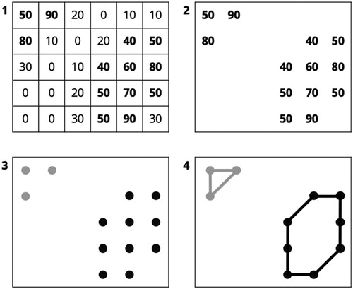
The calculation of the concave hull warrants some additional explanation because, except for a QGIS plugin that first clusters points using a k nearest neighbours’ algorithm, there are to our knowledge no lightweight Python libraries available only considering a set of points as input and producing a concave hull. We, therefore, use our own concave hull algorithm to identify the boundaries of our clusters of points. Although we employ a similar strategy as existing algorithms (e.g. Moreira & Santos, 2007), our method is optimised for our current data model. For each cluster identified in the previous step, we start by creating a list with all unique x-coordinates. The list is first used to create a dictionary of key, value pairs with the unique x-coordinates as keys and with x-coordinate specific y-coordinates as values. We then order the list ‘from east to west’ and loop through it while we use our dictionary to record all the minimum and maximum y-coordinates, respectively. By acquiring first all maximum y-coordinates for all unique x-coordinates and subsequently acquiring all minimum y-coordinates for all unique x-coordinates sorted in reverse order, we effectively extract the border of our clusters of points. The specific order in which the algorithm goes through the points, also ensures that the points are sorted and can be easily transformed into, for instance, a GeoJSON linestring or polygon.

4. Interactive display of surnames distributions

4.1. Website infrastructure

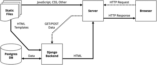
To display the calculated surname distributions onto a website, we link the PostgreSQL database with the calculated surname distributions to a Django framework. Django is an open-source, modern high-level Python web framework that reduces the complexity of setting up a database-driven website. A typical browser request through this setup is illustrated in Figure 3. The moment a user requests the data for a particular surname, the browsers sends a request to the Django backend. Django evaluates this request, and if all is fine, it retrieves the data from the PostgreSQL server. Once the data have been retrieved, our custom Python script is called to reconstruct the grid and extract a vector polygon. Django returns the vectorised data, together with an HTML template, to the server before it is displayed in the browser. This means we have a dynamic website where the content is pulled from the database only when needed and displayed by inserting the content into the basic HTML template. Lastly, we use Bootstrap 4 as a front-end library to style the website and to ensure that the website is fully functional on mobile devices. PostgreSQL, Django, Python and Bootstrap are all open source.

Figure 3. Web application with Django backend. Adapted from: Mozilla (2019).

The alpha version of the KDE visualisation that we have created is, in essence, a rewrite of the Great Britain’s names online database project using a modern, responsive framework, with a completely new database, and greatly expanded data set covering both historic and contemporary Great Britain. The alpha version of the website can be found and accessed through https://data.cdrc.ac.uk/gbnames/.

4.2. Data visualisation

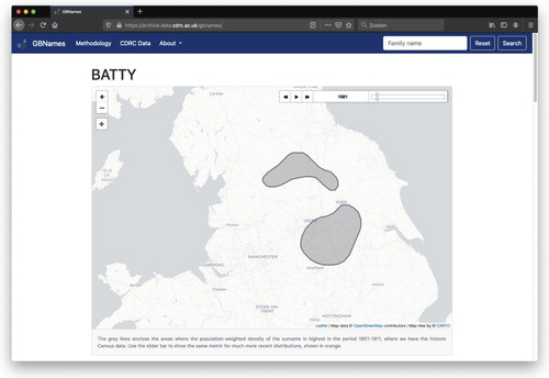
Figure 4 shows a screenshot of the website, after a search on the surname ‘Batty’. The density contour (extracted from the KDE) is shown on a simple OpenStreetMap background – the maps are facilitated by Leaflet.js, a light-weight JavaScript mapping library. By using the slider bar, users can go through the subsequent years for which data are available and interactively see the density contours of the surname remain stable or change over time.

Figure 4. KDE density contours for ‘Batty’ in 1881.

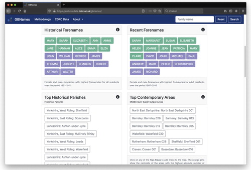
Below the density contours, selected surname statistics are displayed. At the moment, we have included the ten most frequent female and male forename pairings in the combined historic data sets (1851–1911) and the combined recent data sets (1997–2016). For the surname ‘Batty’, for instance, the names ‘Sarah’, ‘Mary’, and ‘Elizabeth’ appear in this top ten in both time periods (Figure 5). Also, the areas, in the form of historic Parishes or the more modern census geography of the Middle Super Layer Output Layer (MSOA), in which the surname is most frequently observed are listed. The centroids of these areas are automatically mapped when clicked on.

Figure 5. Surname-specific frequency statistics.

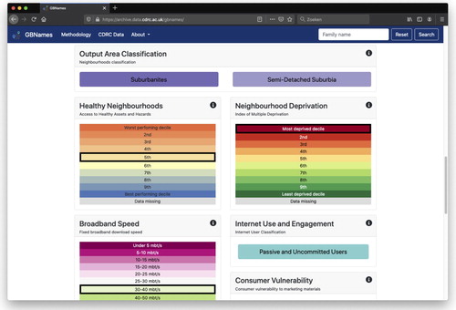
Besides the location and forenames, we link the surname searches to some existing consumer indices produced by the Consumer Data Research, specifically to the Access to Healthy Assets and Hazard (AHAH) index, the Output Area classification, broadband speed, internet usage, and deprivation index. These data sets are available as open data or for bona fide research purposes on successful application by accredited safe researchers to the UK Economic and Social Research Council Consumer Data Research Centre (https://www.cdrc.ac.uk/). For each surname, these indicators are calculated for the most recent data set based on the modal or average score. For instance, in 2016, individuals with the surname ‘Batty’ lived in an output area classified as ‘Suburbanites’ [Figure 6]. In essence, for every surname in our database, we created a small surname profile specific to that surname showing modal or average scores that related to its bearers.

Figure 6. Surname-specific consumer statistics.

5. Discussion

5.1. Processing and dynamically visualising large population data sets

We have introduced a method to create a database with approximately 1.2 million surname distributions for six years of historic census data and 20 years of contemporary Consumer Registers. We showed that the methodology that we developed to compress, and store raster grids makes it feasible to create a database that is linked to a modern, dynamic website which can display surname geographies over time as well as surname-specific surname profiles.

Powered by a completely new database that, to our knowledge, hosts the largest ever collection of surname distributions in Great Britain, the fully re-designed ‘GBNames’ website allows for the easy dissemination of surname research to a wider audience. We have shown how a large data set comprising of individual-level data can be effectively processed and augmented with interesting metrics. The focus on individual surnames allows for the exploration of the changing nature of these spatial data. A major advantage of this method is that the website at no point requires a connection to the database that holds the sensitive individual-level data. Also, even though we are working with a very large data set, we have shown that for large-scale calculations one does not necessarily have to move to software specifically developed to deal with Big Data problems such as distributed computing solutions like Hadoop and Spark. Lastly, the implementation of a custom data compression solution also ensures that the size of the final database is relatively modest.

Besides visualisation, the calculated surname distributions can also potentially be used in the development of a place-based perspective of population change (with a high temporal granularity for the past 20 years). For instance, we hope to consider whether faster declines in the shares of long-established populations of local surname bearers are associated with other demographic characteristics, such as higher levels of neighbourhood population churn, different community structures or distinctive patterns of economic activity. The granularity of the database also allows us to consider a large scale application to study neighbourhood structure (cf. Longley et al., 2007) and population change (cf. Van Dijk & Longley, 2020). Particularly interesting would be to start identifying how these individual surname geographies contribute to the composition of places, to what extent places are constituted by different surname structures, and to what extent a place-based surname hierarchy exists – a ‘name-based central place theory’ – and places and locations can be profiled in terms of their demography.

5.2. Performance

The calculation of thousands of KDEs is highly computationally intensive and therefore could not be implemented through an ‘on the fly’ calculation following every user request. Even if this were to be possible, for privacy reasons we cannot connect a database with individual-level data to a public-facing website. Although we do not have exact benchmarks, the full implementation of the sequence of retrieving the data, calculating the KDEs, and saving the resulting KDE contours would take months to complete without optimisation and parallelisation. Using specialised tools for communication with the databases (psql) and using a separate script for the KDE calculation (R), speeds up the process significantly but given the large number of surnames would still be infeasible. The final solution made use of a high-performance Linux cluster that allowed for the simultaneous calculation of approximately 250 KDEs. Using this approach enabled he full calculation of the KDEs for all surnames to be completed in approximately eight days.

On the client-side, retrieval of the KDE contours varied between surnames – with surnames that are more widespread and had longer contours as well as surnames that occurred in all years taking more time to process. In some cases, surnames searches can take up to 60 seconds to be executed. The relatively time-consuming part is the grid reconstruction of the individual KDEs, with large contours for each year sometimes taking up to five seconds from being requested from the server to being displayed onto the map. To mitigate this problem, the raster grids of the 10,000 most frequent surnames have been pre-constructed and saved in a separate database – even high-frequency surnames that are widespread, such as Smith, are now fully retrieved and displayed within two seconds. Moreover, once a user initiates a search for a surname that is not present in our pre-rendered database, the outcome of the calculations is automatically saved in order to facilitate quick retrieval for any future searches on its subject name.

5.3. Limitations

Being able to store a large number of KDEs without having to pre-determine the contour levels offers some flexibility on the side of the analysis, however, the bandwidth used to calculate the KDE in the first place cannot be adjusted. If there are concerns about how the bandwidth is calculated, the entire process will have to be repeated. Careful parametrisation of the KDE calculation is therefore crucial. Also, there are some concerns stemming from the commercial nature of the Consumer Registers. The sources of the data are of unknown provenance and there is likely some unevenness in their coverage. However, by triangulating these Consumer Registers with data from the Office for National Statistics, for instance with Mid-Year Population Estimates (Lansley et al., 2018), and by developing heuristics and procedures for internal validation and linkage (Lansley et al., 2019), they are the best available source of contemporary individually georeferenced records.

5.4. Concluding remarks

We have demonstrated a novel way in which scale-free surname distributions of a large number of cases can be effectively calculated, stored, and retrieved. This makes it possible to make individual visualisations of surname geographies coupled with surname-specific consumer statistics available to the general public. At the same time, our method keeps the integrity of the calculated surname distributions intact. As such, the value of our method is that the same data set can be used for the study of intergenerational demographic change and stasis, social mobility, and insights into processes of contagious and hierarchical diffusion of local populations.

Software

The calculation of the KDEs requires bash (Unix shell) to enable parallel processing with GNU Parallel, the R programming language (with the ‘Sparr’ library), and PostgreSQL. The website was subsequently built by using the Python-based open-source web framework Django, JavaScript (including ‘jQuery’ and mapping library ‘Leaflet.js’), HTML, and CSS (in combination with front-end framework Bootstrap 4).

Disclosure statement

No potential conflict of interest was reported by the author(s).

Additional information

Funding

This work is supported by the UK ESRC Consumer Data Research Centre (CDRC) grant reference ES/L011840/1 and EPSRC grant EP/M023583/1 (‘UK Regions Digital Research Facility’).

References

- Bates, D., & Maechler, M. (2018). Matrix: Sparse and dense matrix classes and methods [R package version 1.2.15]. https://cran.r-project.org/package=Matrix
- Bloothooft, G., & Darlu, P. (2013). Evaluation of the Bayesian method to derive migration patterns from changes in surname distributions over time. Human Biology, 85(4), 553–568. https://doi.org/10.3378/027.085.0403
- Carlos, H. A., Shi, X., Sargent, J., Tanski, S., & Berke, E. M. (2010). Density estimation and adaptive bandwidths: A primer for public health practitioners. International Journal of Health Geographics, 9(1), 39 https://doi.org/10.1186/1476-072X-9-39
- Cheshire, J. (2014). Analysing surnames as geographic data. Journal of Anthropological Sciences, 92, 99–117. https://doi.org/10.4436/JASS.92004
- Cheshire, J., & Longley, P. A. (2012). Identifying spatial concentrations of surnames. International Journal of Geographical Information Science, 26(2), 309–325. https://doi.org/10.1080/13658816.2011.591291
- Cheshire, J., Longley, P. A., & Singleton, A. D. (2010). The surname regions of Great Britain. Journal of Maps, 6(1), 401–409. https://doi.org/10.4113/jom.2010.1103
- Corwin, J., Silberschatz, A., Miller, P. L., & Marenco, L. (2007). Dynamic tables: An architecture for managing evolving, heterogeneous biomedical data in relational database management systems. Journal of the American Medical Informatics Association, 14(1), 86–93. https://doi.org/10.1197/jamia.M2189
- Davies, T. M., Marshall, J. C., & Hazelton, M. L. (2018). Tutorial on kernel estimation of continuous spatial and spatiotemporal relative risk. Statistics in Medicine, 37(7), 1191–1221. https://doi.org/10.1002/sim.7577
- Degioanni, A., & Darlu, P. (2001). A Bayesian approach to infer geographical origins of migrants through surnames. Annals of Human Biology, 28(5), 537–545. https://doi.org/10.1080/03014460110034265
- Higgs, E., & Schürer, K. (2014). Integrated Census Microdata (I-CeM), 1851-1911 [data collection]. UK Data Service. https://doi.org/10.5255/UKDA-SN-7481-1
- Jobling, M. A. (2001). In the name of the father: Surnames and genetics. Trends in Genetics, 17(6), 353–357. https://doi.org/10.1016/S0168-9525(01)02284-3
- Kandt, J., Cheshire, J. A., & Longley, P. A. (2016). Regional surnames and genetic structure in Great Britain. Transactions of the Institute of British Geographers, 41(4), 554–569. https://doi.org/10.1111/tran.12131
- Kandt, J., Van Dijk, J., & Longley, P. A. (2020). Family name origins and inter-generational demographic change in Great Britain. Annals of the American Association of Geographers. https://doi.org/10.1080/24694452.2020.1717328.
- Lan, T., Kandt, J., & Longley, P. A. (2018). Ethnicity and residential segregation. In P. A. Longley, A. Singleton, & J. A. Cheshire (Eds.), Consumer data research (pp. 71–83). UCL Press.
- Lan, T., & Longley, P. A. (2019). Geo-referencing and mapping 1901 census addresses for England and Wales. ISPRS International Journal of Geo-Information, 8(8), 320. https://doi.org/10.3390/ijgi8080320
- Lansley, G., Li, W., & Longley, P. A. (2018, April 17–20). Modelling small area level population change from administrative and consumer data. Proceedings of the 26th Conference on GIS Research UK (GISRUK), Leicester: University of Leicester.
- Lansley, G., Li, W., & Longley, P. A. (2019). Creating a linked consumer register for granular demographic analysis. Journal of the Royal Statistical Society: Series A (Statistics in Society), 182(4), 1587–1605. https://doi.org/10.1111/rssa.12476
- Longley, P. A., Webber, R., & Lloyd, D. (2007). The quantitative analysis of family names: Historic migration and the present day neighborhood structure of Middlesbrough, United Kingdom. Annals of the Association of American Geographers, 97(1), 31–48. https://doi.org/10.1111/j.1467-8306.2007.00522.x
- Mateos, P., Longley, P. A., & O’Sullivan, D. (2011). Ethnicity and population structure in personal naming networks. PLoS ONE, 6(9), e22943. https://doi.org/10.1371/journal.pone.0022943
- McKinney, W. (2010, June 28–July 3). Data structures for statistical computing in Python. Proceedings of the 9th Python in Science Conference. ( pp. 51–56).
- Moreira, A., & Santos, M. Y. (2007, March 7–11). Concave hull: A k-nearest neighbours approach for the computation of the region occupied by a set of points. Proceedings of GRAPP 2007 - 2nd international conference on computer graphics theory and applications ( pp. 61–68), Setúbal: GRAPP. https://doi.org/10.5220/0002080800610068
- Mozilla. (2019). Introduction to the server side. Retrieved April 8, 2019, from https://developer.mozilla.org/en-US/docs/Learn/Server-side/First_steps/Introduction
- Pedregosa, F., Varoquaux, G., Gramfort, A., Michel, V., Thirion, B., Grisel, O., … Duchesnay, É. (2011). Scikit-learn: Machine learning in Python. Journal of Machine Learning Research, 12, 2825–2830.
- R Core Team. (2018). R: A language and environment for statistical computing. R Foundation for Statistical Computing.
- Schürer, K., Penkova, T., & Shi, Y. (2015). Standardising and coding birthplace strings and occupational titles in the British Censuses of 1851 to 1911. Historical Methods: A Journal of Quantitative and Interdisciplinary History, 48(4), 195–213. https://doi.org/10.1080/01615440.2015.1010028
- Shi, X. (2010). Selection of bandwidth type and adjustment side in kernel density estimation over inhomogeneous backgrounds. International Journal of Geographical Information Science, 24(5), 643–660. https://doi.org/10.1080/13658810902950625
- Singleton, A. D., Longley, P. A., Allen, R., & O’Brien, O. (2011). Estimating secondary school catchment areas and the spatial equity of access. Computers, Environment and Urban Systems, 35(3), 241–249. https://doi.org/10.1016/j.compenvurbsys.2010.09.006
- Soundararaj, B., Cheshire, J., & Longley, P. A. (2019, April 23–26). Medium data toolkit - A case study on smart street Sensor project. Proceedings of the 27th conference on GIS Research UK (GISRUK), Newcastle: Newcastle University.
- Tange, O. (2011). GNU Parallel - The command-line power tool. Login: The USENIX Magazine, 36(1), 42–47.
- Van Dijk, J., Lansley, G., Lan, T., & Longley, P. A. (2019, April 23–26). Using the spatial analysis of family names to gain insight into demographic change. Proceedings of the 27th conference on GIS Research UK (GISRUK), Newcastle: Newcastle University.
- Van Dijk, J., & Longley, P. A. (2020). Platial geo-temporal demographics using family names. In R. Westerholt, & F.-B. Mocnick (Eds.), Proceedings of the 2nd international symposium on platial information science (PLATIAL'19) (pp. 23–31). Warwick University. https://doi.org/10.5281/zenodo.3628863
- Zhang, G., Zhu, A.-X., & Huang, Q. (2017). A GPU-accelerated adaptive kernel density estimation approach for efficient point pattern analysis on spatial big data. International Journal of Geographical Information Science, 31(10), 2068–2097. https://doi.org/10.1080/13658816.2017.1324975