Exposure to landslides in rural areas in Central Italy

ABSTRACT

Starting on 24th August 2016, Central Italy was struck by a six-month earthquake sequence that caused 303 victims and extensive major damages to urban areas and infrastructures, in some cases entire villages needed complete rebuilding. In this paper we present a map that portrays the overall susceptibility to multiple landslide types and the exposure to landslides of the rural-urban areas of the Castelsantangelo sul Nera Municipality, a typical village of the central Italian Apennine. The map is based on a procedure that ingests geomorphological data and models and groups the individual landslide susceptibility maps in a joint susceptibility and exposure map based on expert-defined criteria. The procedure has been applied to built-up and to undeveloped areas to highlight their exposure and was used as a tool for planning post-seismic reconstruction. We advise that such maps are used also as basic tool for ordinary urban planning.

KEYWORDS:

• Debris-flow
• rockfall
• shallow and deep-seated slide
• landslide susceptibility
• exposure to landslides
• post-seismic reconstruction

1. Introduction

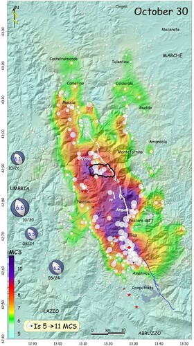
In 2016, Central Italy was struck by a six-month seismic sequence, started on 24 August. The sequence was characterised by two main shocks in August 2016 (Mw 6.0 and Mw 5.4), three major shocks (Mw 5.4, 5.9 and 6.5) in October 2016, and four shocks with Mw between 5.0 and 5.5 in January 2017. The sequence was characterised by more than 50,000 aftershocks in the first four months (Santangelo et al., 2019; Vignaroli et al., 2019). The earthquakes caused a total of 303 casualties, thousands of homeless, and severe damages to hundreds of villages, mostly located in the central Apennines. In 29 villages the macroseismic intensity was higher than IX degree of the Mercalli-Cancani-Sieberg (MCS) intensity, and for 5 of them it reached XI degree MCS (Figure 1; Galli et al., 2017). In some cases, entire villages were destroyed and needed partial or even complete re-building.

Figure 1. Cumulative effects of the 24th August and 26th and 30th October earthquakes. Red stars, 2016–2017 Ml > V events. Red diamond, macroseismic epicentre. Blue line, active fault segments of the Laga Mounts (dotted if inferred). White line, Mount Vettore fault system, responsible for the 2016 earthquakes (dotted if inferred). Modified after Galli et al. (2017). Black outlined polygon, study area of this work.

In the immediate aftermath of the first seismic event, several requests were raised by the National Department of Civil Protection (DPC) to identify sites for temporary settlements and define landslide residual risk conditions on roads (Santangelo et al., 2019). In the emergency and immediate post-emergency phases, the DPC requested to identify suitable areas for reconstruction or relocation of damaged or destroyed urban areas.

The zonation of landslide susceptibility, hazard and risk in urban areas is a task that has been addressed in different ways by the scientific community at different scales. Such mapping activities, however, were usually carried out by considering single landslide types (e.g. Carrara et al., 2008; Frattini et al., 2008; Reichenbach et al., 2018). Therefore, defining the susceptibility or the potential expected interaction of landslides with urban areas for multiple landslide types at the catchment scale is yet an open problem.

The DPC request was answered by designing an expeditious procedure aimed at integrating (i) geomorphological analyses carried out in the field, (ii) expert stereoscopic aerial photo-interpretation and (iii) susceptibility models for rockfalls (Guzzetti et al., 2002b), debris-flows (Mergili et al., 2015) and shallow and deep-seated slides (Cardinali et al., 2002; Reichenbach et al., 2018).

The procedure is based on (i) a heuristic geomorphological model for shallow (SL) and deep-seated (DL) landslides of the slide type, (ii) two conceptual models to define areas potentially affected by debris-flows (DF), (iii) a distributed physically based model to delineate the rockfall (RF) runout areas. The outputs of the models were then combined to define the overall susceptibility and exposure to landslide hazards of areas with morphological characteristics similar to selected built-up areas.

Despite the expeditious approach, the procedure is thought to be general and applicable to evaluate the landslide susceptibility conditions and exposure of (i) built-up damaged areas, (ii) destroyed areas to be relocated, and (iii) undeveloped areas within which to relocate the destroyed centres, or parts of them. Despite the specific areas to which it was applied, the procedure is not specific or limited to such areas but is general and may be applied to other areas where similar answers must be given in a limited amount of time.

2. Study area

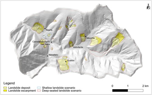
The analyses focus on the main hamlet of the municipality of Castelsantangelo sul Nera, located on the right bank of the Nera River and the five villages of Macchie, Nocelleto, Nocria, and Vallinfante (Main Map). The total area investigated is 28.75 km². Like other villages in the Italian Apennines, several built-up areas in the study area occupy areas potentially exposed to different landslide types. The village of Castelsantangelo sul Nera has been historically hit by debris-flows, and an important event was registered on 27 July 1906 (Guzzetti et al., 2002a). In the upper part of the catchment of the Nera River, large debris-flows are widespread (Arignoli et al., 2007; Guzzetti & Cardinali, 1991) many of which showing evidences of recent morphological evolution. The hamlets of Vallinfante and Macchie are located close to such large debris-flows (Arignoli et al., 2007). Also, earth- and rock-slides and rockfalls are common phenomena in this area (Map B in Main Map).

3. Data and methods

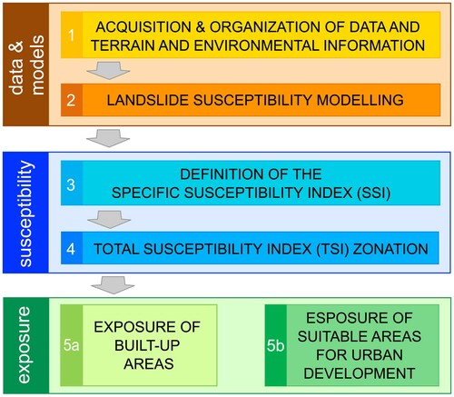
A six-step procedure was designed to define the level of susceptibility of the studied areas (Figure 2). The procedure uses data available or acquired ad-hoc and returns a semi-quantitative assessment of the degree of exposure to landslides. The procedure applies both to classify the exposure of built-up areas, and to identify suitable areas for urban development. The procedure considers only rockfalls, debris-flows, shallow and deep-seated slides.

Figure 2. Logical-functional model of the procedure.

Time and information available for the survey were scarce, due to the emergency conditions. Therefore, due to the complexity of the instability phenomena to be investigated, and the extent of the area (Main Map), the issue was addressed through an expeditious and expert-based procedure, based on empirical knowledge and understanding of present phenomena and processes.

3.1. Data acquisition

The first step consists in the acquisition of already published data or of new input data used by the procedure.

3.1.1. Digital elevation model

We used the Digital elevation model (DEM) TINITALY, produced from several information sources (Tarquini et al., 2012, 2007) and distributed by the National Institute of Geophysics and Volcanology (INGV). The DEM has a ground sampling distance of 10 m. In the study area, the DEM was produced starting from the Technical Regional Cartography (CTR), a topographic map at 1:10,000 scale, which was obtained from aerial photographs acquired in May–June 2000.¹ This should be considered the temporal reference of the TINITALY in this area.

3.1.2. Aerial photographs

To produce the landslides inventory map, two sets of stereoscopic aerial photographs (APs) were used. APs were taken (i) in 1955, in black and white, at a scale of about 1:33,000, and (ii) in October 1997, in black and white, at a scale of about 1:20,000.

3.1.3. Landslide inventory map

The landslide inventory map (LIM) has been prepared through photointerpretation of APs adopting well-established photointerpretation method and criteria (Cardinali et al., 2000; Fiorucci et al., 2018; Guzzetti et al., 2012; Santangelo et al., 2014). Among the ancillary material usually consulted to prepare LIMs (landcover/land-use maps, other LIMs, geological maps), it is worth mentioning the geomorphological map of the Marche Region, freely accessible online.² The map has been published at 1:10,000 scale and contains many useful and detailed information on tectonics, hydrography, gravity-driven morphologies, fluvial and fluvial-glacial morphologies, anthropic morphologies.

Aerial photo interpretation was verified through targeted field checks. The information on landslides in the LIM are used (i) directly, to identify the areas where landslides are present and have been recognised and (ii) indirectly, as input for susceptibility models and for the definition of landslides evolutionary scenarios.

In the LIM (Map A in Main Map), the main types of landslides are represented by shallow and deep-seated slides, debris-flows and rockfalls (Cruden & Varnes, 1996; Hungr et al., 2014).

3.2. Landslide susceptibility modelling

The second step of the procedure consisted in classifying the propensity of the territory to be affected by rockfalls, debris-flows, and landslides (2 in Figure 2).

3.2.1. Rockfalls

To model the susceptibility to rockfall phenomena, the software STONE (Guzzetti et al., 2002b) was used. To simulate the physical process of rockfall, STONE implements a ‘lumped mass’ approach in which potential boulders are considered without dimensions and with the mass concentrated in the centre of mass. STONE performs a kinematic simulation of the falling boulder. To carry out the simulation, STONE needs the definition of (i) the possible rockfall source areas, (ii) the number of boulders falling from each source area, (iii) the initial speed and the boulder release angle, (iv) a speed threshold below which the boulder stops. In addition to these parameters, STONE needs (v) a DEM that describes the topography of the study area, and (vi) the coefficients of dynamic friction, and of normal and tangential restitution at impact points.

The source areas passed to the model were defined as all the pixels of the DEM which slope is greater than 50° according to the evidences collected in the field during the emergency and post-emergency activities in the area hit by the 2016 seismic sequence in central Italy (Santangelo et al., 2019).

STONE considers the uncertainty inherent in the input data and in the simulation by (i) ‘launching’ a variable number of boulders from each source area cell, and (ii) randomly varying the horizontal release angle, the dynamic rolling friction and the normal and tangential restitution coefficients. Using GIS technologies, STONE computes the rockfall trajectories of individual boulders simulated in three dimensions, and outputs three raster maps which report for each pixel (i) a frequency map which reports the number of trajectories, (ii) the maximum speed, and (iii) the maximum elevation from the ground.

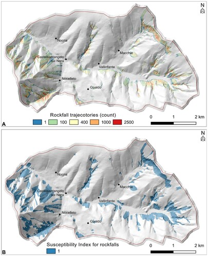
The three raster maps can, in turn, be used to define rockfall hazard levels (Guzzetti et al., 2004; Santangelo et al., 2019). In this work, we reclassified the frequency map output by STONE (Figure 3(A)) in two classes only to define the area where a rockfall runout is predicted, neglecting the value of frequency (Figure 3(B)). This led to a binary map (0, 1) that distinguishes areas where rockfalls are not expected (0) from areas where rockfalls are expected (1). The binary map so defined is referred to as map of the Susceptibility Index (SI) for rockfalls (Map B in Main Map).

Figure 3. (A) Map of the number of rockfall trajectories modelled in the area of Castelsantangelo sul Nera. (B) Map of the Susceptibility Index for rockfalls.

3.2.2. Debris-flows

Susceptibility to debris-flows was modelled following an approach based on the application of conceptual models. Unlike physically based models, conceptual models do not aim at reproducing the physical processes underlying the debris-flows phenomena but use simplified empirical relationships. Conceptual models allow working out the problem of lack of data on the mechanical and physical characteristics of the materials involved in the processes.

Two conceptual models were used to delineate the areas susceptible to debris-flow runouts: (i) the Modified Single Flow Direction (MSF) model (Huggel et al., 2003), and (ii) the r.randomwalk model (Mergili et al., 2015).

MFS is a conceptual model for the study of mass movements that can be implemented in a GIS (Gruber et al., 2009). The model requires: (i) the location of the starting points of debris-flows, and (ii) a DEM. A linear function is coupled to the single-flow algorithm to enabling flow diversion in low-slope areas. The result of the model is an expeditious prediction of the areas potentially affected by debris-flow runout expressed in probability-related values. The debris-flow runout distance is determined based on empirical data on average slope trajectories.

The conceptual model ‘r.randomwalk’ (Mergili et al., 2015) is implemented in a software developed to operate in GRASS GIS (GRASS Development Team, 2017). The model randomly simulates the paths of debris-flows started from known (pre-defined) release sources, which can be punctual or areal. The random trajectories are conditioned by the local topography (DEM) but are forced not to concentrate along linear paths. The trajectories end when a predefined ‘break criterion’ is met. Several break criteria can be used, which are mostly based on empirical relationships of the reach angles defined in the literature (Haeberli, 1983; Huggel et al., 2003; Perla et al., 1980; Rickenmann, 1999; Scheidegger, 1973). In this study, the stop condition for each trajectory consisted in a random sample extracted from the distribution of the reach angles observed in the debris-flow deposits reported in the LIM.

For the MSF model, the source areas have been identified by combining the information of the landslide inventory map (Map A in Main Map) with a morphometric approach based on the empirical relationship between the local slope and the contributing area (Cavalli et al., 2017; Wichmann & Becht, 2005; Zimmermann et al., 1997). For the r.randomwalk model, instead, the debris-flow trajectories were simulated starting from each cell of the 10 m DEM within the source areas mapped in the LIM (Map A in Main Map). In both cases, two maps of areas potentially affected by debris-flows were produced.

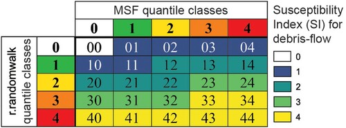
The two maps output by the models were classified according to the values of the quartiles of the distribution of the probability-related values in case of MSF model and of the trajectories number in case of r.randomwalk: 0 (null), 1 (low, 0% – 1st quartile), 2 (medium, 1st quartile – 2nd quartile), 3 (high, 2nd quartile – 3rd quartile), 4 (very high, 3th quartile – 4th quartile). The reclassified maps are shown in Figure 4(A, B). To define a joint model, the two maps were combined according to a two-digit positional index (Figure 4(C)) in which the values of the MSF and of the r.randomwalk reclassified maps are concatenated starting from the left. Finally, to produce the susceptibility map for debris-flow, we classified the map of the positional index (Figure 4(C)) in a five classes map (Figure 4(D)) ranging from 0 to 4 according to the expert-based criteria illustrated in Figure 5. Additionally, to give more weight to the geomorphological evidences, the final map for debris-flows assumes the maximum value (4) where debris-flows were mapped in the LIM.

Figure 4. Maps produced to define debris-flow susceptibility. Reclassified output maps of the MSF (A) and r.randomwalk (B) models. Index derived by combining the outputs of the models in A and B (C). Map of the Susceptibility Index for debris-flows (D). Grouping criteria are illustrated in Figure 5.

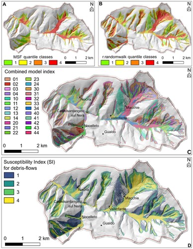
Figure 5. Criteria used to group the 25 possible values of the positional index used to combine the debris-flows model outputs. Colours correspond to those used in Figure 4(A, B) for the model classes and to Figure 4(D) for the groups colours.

The map so defined is referred to as map of the Susceptibility Index for debris-flows (Map C in Main Map).

3.2.3. Shallow and deep-seated landslides

For the study area, the susceptibility to landslides of the slide type was defined according to a heuristic procedure that identifies the possible ‘landslide scenarios’ as defined by Cardinali et al. (2002, p. 65). Such scenarios were delineated through the visual interpretation of stereoscopic APs (Cardinali et al., 2002). The method requires the expert identification of landslide scenarios, that is the estimation (in case of partial or total re-mobilisation of existing landslides, or in case of the occurrence of new landslides) of the possible propagation, retrogression and lateral expansion distance of single landslide movements, or of groups of landslides showing similar type of movement (Figure 6). In each scenario, evaluations are based on the morphology of the slope, and local geo-lithological conditions and past landslides information extracted from the landslide inventory.

Figure 6. Landslide scenarios for deep-seated and shallow landslides of the slide type.

The scenarios are collected in two binary maps, one for deep-seated landslides (Map D in Main Map) and one for shallow landslides (Map E in Main Map), in which values 0 and 1 indicate the absence or presence of landslide scenarios, respectively. The so defined maps are referred to as maps of the Susceptibility Index for deep-seated and shallow landslides.

3.3. Specific Susceptibility Index

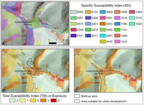
To describe the susceptibility of each pixel to different landslide types, the four Susceptibility Indices have been concatenated into a four-digit positional index, named Specific Susceptibility Index (3 in Figure 2, and Table 1 in Main Map). In the SSI, from left to right, each digit replicates the Susceptibility Indices for (i) rockfalls, (ii) debris-flows, (iii) deep-seated landslides, and (iv) shallow landslides. Based on the definition given to the SIs, the SSI has 40 different values (Table 1 in Main Map), one for each of the possible combinations of the Susceptibility Indices. Figure 7(A) shows a detail of the SSI map for the village of Castelsantangelo sul Nera.

Figure 7. Detail of the main hamlet of Castelsantangelo sul Nera. Specific Susceptibility Index (A), and Total Susceptibility and exposure map compared to built-up areas (B) and to areas suitable for urban development (C).

3.4. Total susceptibility zonation

The fourth step of the procedure (4 in Figure 2) consists in defining criteria to group the 40 values of SSI in classes to operate a susceptibility zonation. Main Map shows the geographic distribution of the Total Susceptibility Index (TSI), a five-class index resulting from the expert-based classification of the SSI. The set of rules based on expert evaluations are illustrated in Table 1 in Main Map.

For each pixel, the TSI is expressed as an integer number between 0 and 4, indicating: 0, negligible; 1, low susceptibility; 2, medium susceptibility; 3, high susceptibility; 4, very high susceptibility. The rationale adopted to group the values of SSI is to assign high TSI where possible life loss is expected (i.e. where fast-moving landslides are expected). Table 1 in Main Map illustrates the correspondence between SIs, SSI and TSI values. The table shows that: (i) one value of SSI corresponds to the value 0 of TSI; (ii) three values of SSI correspond to the value 1 of TSI; (iii) six values of SSI correspond to the value 2 of TSI; (iv) eighteen values of SSI correspond to the value 3 of TSI; (v) twelve values of SSI correspond to the value 4 of TSI.

3.5. Exposure

The fifth and sixth steps of the procedure (5a and 5b in Figure 2) consist in identifying the exposure to the considered landslide types of (a) the built-up areas and (b) areas potentially suitable for urban development.

UNISDR (2009) defines the ‘exposure’ as ‘People, property, systems, or other elements present in hazard zones that are thereby subject to potential losses’. Based on this definition, we consider as ‘exposed’ all structures, infrastructures and people that are located (built-up areas, 5a in Figure 2) or might be located (areas suitable for urban development, 5b in Figure 2) in areas susceptible to landslides, that is where the TSI is greater than 0.

Consequently, the levels of exposure of urbanised areas (or of areas suitable for urban development) are the same as the Total Susceptibility Index.

3.6. Criteria for defining suitable areas for urban development

Arguably, not all places with low or negligible susceptibility are suitable for urban development. For example, they must be excluded if the slope or the elevation is too high compared to the local urban areas, or if the areas are too small. Therefore, to fulfil the request of DPC of defining areas potentially suitable for post-seismic reconstruction, the zonation map of TSI and exposure was coupled to other morphometric constraints. In particular:

1. The first criterion considers as suitable the areas where the exposure is at worst ‘high’ (class 0–3 in Main Map). Areas with very high exposure are considered unconditionally unsuitable (class 4, red in Main Map).

2. The second criterion identifies land parcels at similar or lower altitudes than those of existing settlements (1000 m a.s.l).

3. The third criterion identifies areas having mean and standard deviation of slope respectively less than 10° and 5° (the average values of the villages of Castelsantangelo sul Nera and Nocelleto). The slope values were computed in a circular kernel with a diameter of 90 m (9 cells), which area corresponds to the average area of the blocks of Castelsantangelo sul Nera (about 6000 m²).

4. Results and discussion

The map described and presented in this work (Main Map) represents a susceptibility zonation to landslides of different types. Based on the definition of exposure given in Section 3.5, the map also represents the levels of exposure of existing structures and infrastructures to the considered phenomena (Figure 7(B)), and the levels of exposure of the areas suitable for urban development (Figure 7(C)).

Inspection of the Main Map shows that only 2.5% (0.74 km²) of the study area is morphologically similar (slope and elevation) to the slopes where the existing hamlets were built and is, thence, considered suitable for urban expansion. Of this 0.74 km², 5.9% (44,000 m²) has very low exposure, 2.4% (17,500 m²) low exposure, 9.5% (70,500 m²) medium exposure, 78.4% (580, 200 m²) high exposure and 3.8% (27,800 m²) very high exposure to landslides. Such figures show that for more than 94% of the morphologically suitable areas, protection measures are necessary in case urban development is planned in such areas, since the territory is classified as susceptible to landslides.

From a geographical point of view, suitable areas are well distributed near the five hamlets, but there are only two areas with very low TSI, which are located far from the main hamlet of Castelsantangelo sul Nera and close only to two of the five hamlets (Gualdo and Nocelleto, Main Map). Therefore, to guarantee continuity with (or at least proximity to) existing urban areas, it seems unavoidable the need to plan urban development in susceptible areas.

This map provides knowledge of the landslides potentially affecting the study area, and it could be used to increase risk awareness and as a basic tool for urban planning, albeit it must be specified here that no information is given about the landslides size and their frequency over time. In addition, it is worth mentioning that to each level of TSI (or exposure), the end-users were provided with a list of potential actions suggested to mitigate the impact of landslides on structure, infrastructures and population. For instance, in an area where the TSI is ‘negligible’ it was suggested to only take care of surface water management, as opposed to areas where TSI is ‘high’, which could mean to be concerned about setting up active/passive protection measures for the landslide types involved. To define such protection measures, arguably, it is mandatory that specific detailed studies should follow at the slope scale to define landslide hazard and eventually design and set up adequate active and/or passive protection measures. Moreover, the identification of sites suitable for post-seismic reconstruction urges the integration with the assessment of flood-prone areas, which is out of the topic of this paper.

The analyses carried out in this work were designed and completed in 15 working days by an interdisciplinary team of 9 people during emergency response activities. The procedure can be applied to different context and areas, provided it is carefully customised based on the available data, models, and types of geomorphological processes. The described heuristic aggregations and classifications illustrated are based on a specific situation. Different expert-based criteria for classifications can be defined (also including decision-makers in the process) to fulfil specific requests.

As described in Sections 3.2 to 3.4, the final map (Main Map) is the result of multiple aggregations and heuristic classifications, which, of course, condition the final values of TSI. Despite the map is easily readable, on the other hand, readers can be misled if unaware of how aggregations and classifications were made. Therefore, it is advised that the map is read jointly to the Susceptibility Index maps for single landslides types.

5. Conclusion

This work presents the results of an integrated approach of geomorphological mapping based on heuristic and statistical modelling of landslide susceptibility carried out for an area in Central Italy which was struck by the seismic sequence started on 24 August 2016. The activities aimed at providing the National Department of Civil Protection with the information to define the areas suitable for post-seismic reconstruction in a rural–urban context.

This map represents a joint susceptibility and exposure map which can ultimately be used by planner or decision-makers. The procedure needs data that can be easily collected but requires high expertise in landslide mapping and heuristic and statistical susceptibility modelling.

The Main Map shows that a large part of the area is morphologically unsuitable for urban development, and that the few suitable areas are in large majority exposed to potential losses due to the possible occurrence of different types of landslides. This is a typical feature of mountainous landscapes, where it is advised that maps like the one presented here are produced not only to support post-emergency activities but also ordinary urban planning.

Software

We used: (i) GRASS GIS for running r.randomwalk, (ii) Procedura-DF ArcGIS® 10.3 Toolbox for identifying potential debris-flow starting points (freely available at https://github.com/HydrogeomorphologyTools/Procedura-DF) (iii) an ad hoc developed Toolbox for ArcGIS® 10.3 for running MSF debris-flow model, (iv) the software STONE for rockfall modelling; (v) QGIS (http://www.qgis.org/) to digitise the landslide inventory map and the scenarios, and to organise and analyse the data and model outputs, (vi) ArcGIS® 10.2.1 to produce the initial layout of the map, and (vii) Adobe® Illustrator® (http://www.adobe.com/products/illustrator/) to assemble the final map for publication and graphical editing.

Acknowledgements

We are grateful to Dr. Paolo Galli for allowing to insert Figure 1 from their article Galli et al. (2017). This work was partially funded by the Italian National Department of Civil Protection. MS, MCR and FB designed the map. MS and IM wrote the paper. MS, MCR and FB prepared the landslide inventory and delineated the scenarios for deep-seated and shallow landslides. IM run the r.randomwalk model for debris-flows. MCV, SC, LM run the MSF model for debris-flows. MA run the STONE model for rockfalls. MS, IM, FB, MCR, FG defined the Susceptibility Indices. All authors checked the paper and the map.

Disclosure statement

No potential conflict of interest was reported by the author(s).

Notes

1 (http://www.regione.marche.it/Regione-Utile/Paesaggio-Territorio-Urbanistica/Cartografia/Repertorio/Cartatecnicanumerica110000).

2 The map is accessible at this link: http://www.regione.marche.it/Regione-Utile/Paesaggio-Territorio-Urbanistica/Cartografia/Repertorio/Cartageomorfologicaregionale10000. The sheets which contain our study area are: 325060, 325070, 325100, 325110.

References

- Arignoli, D., Farabollini, P., Gentili, B., Materazzi, M., & Pambianchi, G. (2007). Climatic influence on slope dynamics and shoreline variations: Examples from Marche region (Central Italy). Géographie Pysique Environ, 1, 1–20. https://doi.org/10.4000/physio-geo.1035
- Cardinali, M., Ardizzone, F., Galli, M., Guzzetti, F., & Reichenbach, P. (2000). Landslides triggered by rapid snow melting: the December 1996–January 1997 event in Central Italy [Paper presentation]. Proceedings Plinius Conference ‘99 (October 14–16). Mediterranean Storms, Bios, Cosenza, Maratea, pp. 439–448.
- Cardinali, M., Reichenbach, P., Guzzetti, F., Ardizzone, F., Antonini, G., Galli, M., Cacciano, M., Castellani, M., & Salvati, P. (2002). A geomorphological approach to the estimation of landslide hazards and risks in Umbria. Natural Hazards and Earth System Science, 2(1/2), 57–72. https://doi.org/10.5194/nhess-2-57-2002
- Carrara, A., Crosta, G., & Frattini, P. (2008). Comparing models of debris-flow susceptibility in the alpine environment. Geomorphology, 94(3-4), 353–378. https://doi.org/10.1016/j.geomorph.2006.10.033
- Cavalli, M., Crema, S., Trevisani, S., & Marchi, L. (2017). GIS tools for preliminary debris-flow assessment at regional scale. Journal of Mountain Science, 14(12), 2498–2510. https://doi.org/10.1007/s11629-017-4573-y
- Cruden, D. M., & Varnes, D. J. (1996). Landslide types and processes (Special Report. pp. 36–75). Landslides: Investigation and Mitigation, Transportation Research Board.
- Fiorucci, F., Giordan, D., Santangelo, M., Dutto, F., Rossi, M., & Guzzetti, F. (2018). Criteria for the optimal selection of remote sensing optical images to map event landslides. Natural Hazards and Earth System Sciences, 18, 405–417. https://doi.org/10.5194/nhess-18-405-2018
- Frattini, P., Crosta, G., Carrara, A., & Agliardi, F. (2008). Assessment of rockfall susceptibility by integrating statistical and physically-based approaches. . Geomorphology, GIS Technology and Models for Assessing Landslide Hazard and Risk, 94, 419–437. https://doi.org/10.1016/j.geomorph.2006.10.037
- Galli, P., Castenetto, S., & Peronace, E. (2017). The macroseismic intensity distribution of the 30 October 2016 earthquake in Central Italy (MW 6.6): Seismotectonic Implications: The 2016 Central Italy earthquake intensity. Tectonics, 36(10), 2179–2191. https://doi.org/10.1002/2017TC004583
- GRASS Development Team. (2017). Geographic resources analysis support system (GRASS GIS) (Version 7.2) [Computer software].
- Gruber, S., Huggel, C., & Pike, R. (2009). Chapter 23 modelling mass movements and landslide susceptibility. In T. Hengl & H. I. Reuter (Eds.), Developments in Soil Science, Geomorphometry (pp. 527–550). Elsevier.
- Guzzetti, F., & Cardinali, M. (1991). Debris-flow phenomena in the Central Apennines of Italy. Terra Nova, 3(6), 619–627. https://doi.org/10.1111/j.1365-3121.1991.tb00204.x
- Guzzetti, F., Cipolla, F., Pagliacci, S., Sebastiani, C., & Tonelli, G. (2002a, January 22–24). Information system on historical landslides and floods in Italy [Paper presentation]. Urban Hazards Forum, New York, p. 13.
- Guzzetti, F., Crosta, G., Detti, R., & Agliardi, F. (2002b). STONE: A computer program for the three-dimensional simulation of rock-falls. Computers & Geosciences, 28(9), 1079–1093. https://doi.org/10.1016/S0098-3004(02)00025-0
- Guzzetti, F., Mondini, A. C., Cardinali, M., Fiorucci, F., Santangelo, M., & Chang, K.-T. (2012). Landslide inventory maps: New tools for an old problem. Earth-Science Reviews, 112(1-2), 42–66. https://doi.org/10.1016/j.earscirev.2012.02.001
- Guzzetti, F., Reichenbach, P., & Ghigi, S. (2004). Rockfall hazard and risk assessment along a transportation corridor in the Nera Valley, central Italy. Environmental Management, 34(2), 191–208. https://doi.org/10.1007/s00267-003-0021-6
- Haeberli, W. (1983). Frequency and characteristics of Glacier Floods in the Swiss Alps. Annals of Glaciology, 4, 85–90. https://doi.org/10.3189/S0260305500005280
- Huggel, C., Kääb, A., Haeberli, W., & Krummenacher, B. (2003). Regional-scale GIS-models for assessment of hazards from glacier lake outbursts: Evaluation and application in the Swiss Alps. Natural Hazards and Earth System Science, 3(6), 647–662. https://doi.org/10.5194/nhess-3-647-2003
- Hungr, O., Leroueil, S., & Picarelli, L. (2014). The Varnes classification of landslide types, an update. Landslides, 11(2), 167–194. https://doi.org/10.1007/s10346-013-0436-y
- Mergili, M., Krenn, J., & Chu, H.-J. (2015). R.randomwalk v1, a multi-functional conceptual tool for mass movement routing. Geoscientific Model Development, 8(12), 4027–4043. https://doi.org/10.5194/gmd-8-4027-2015
- Perla, R., Cheng, T. T., & McClung, D. M. (1980). A Two–parameter model of snow–avalanche motion. Journal of Glaciology, 26(94), 197–207. https://doi.org/10.3189/S002214300001073X doi: 10.1017/S002214300001073X
- Reichenbach, P., Rossi, M., Malamud, B. D., Mihir, M., & Guzzetti, F. (2018). A review of statistically-based landslide susceptibility models. Earth-Science Reviews, 180, 60–91. https://doi.org/10.1016/j.earscirev.2018.03.001
- Rickenmann, D. (1999). Empirical relationships for debris flows. Natural Hazards, 19(1), 47–77. https://doi.org/10.1023/A:1008064220727
- Santangelo, M., Alvioli, M., Baldo, M., Cardinali, M., Giordan, D., Guzzetti, F., Marchesini, I., & Reichenbach, P. (2019). Brief communication: Remotely piloted aircraft systems for rapid emergency response: Road exposure to rockfall in Villanova di Accumoli (central Italy). Natural Hazards and Earth System Sciences, 19(2), 325–335. https://doi.org/10.5194/nhess-19-325-2019
- Santangelo, M., Gioia, D., Cardinali, M., Guzzetti, F., & Schiattarella, M. (2014). Landslide inventory map of the upper Sinni River valley, Southern Italy. Journal of Maps, 0, 1–10. https://doi.org/10.1080/17445647.2014.949313
- Scheidegger, A. E. (1973). On the prediction of the reach and velocity of catastrophic landslides. Rock Mechanics, 5(4), 231–236. https://doi.org/10.1007/BF01301796
- Tarquini, S., Isola, I., Favalli, M., Mazzarini, F., Bisson, M., Pareschi, M. T., & Boschi, E. (2007). TINITALY/01: A new triangular irregular network of Italy. Annals of Geophys, 50, 407–425. https://doi.org/10.4401/ag-4424
- Tarquini, S., Vinci, S., Favalli, M., Doumaz, F., Fornaciai, A., & Nannipieri, L. (2012). Release of a 10-m-resolution DEM for the Italian territory: Comparison with global-coverage DEMs and anaglyph-mode exploration via the web. Computers & Geosciences, 38(1), 168–170. https://doi.org/10.1016/j.cageo.2011.04.018
- UNISDR. (2009). UNISDR terminology on disaster risk reduction. UNDRR.
- Vignaroli, G., Mancini, M., Bucci, F., Cardinali, M., Cavinato, G. P., Moscatelli, M., Putignano, M. L., Sirianni, P., Santangelo, M., Ardizzone, F., Cosentino, G., Salvo, C. D., Fiorucci, F., Gaudiosi, I., Giallini, S., Messina, P., Peronace, E., Polpetta, F., Reichenbach, P., … Stigliano, F. (2019). Geology of the central part of the Amatrice Basin (Central Apennines, Italy). Journal of Maps, 15(2), 193–202. https://doi.org/10.1080/17445647.2019.1570877
- Wichmann, V., & Becht, M. (2005). Modeling of geomorphic processes in an Alpine catchment. In P. M. Atkinson, G. M. Foody, S. E. Darby, & F. Wu (Eds.), Geodynamics (pp. 151–167). CRC Press.
- Zimmermann, M., Mani, P., & Romang, H. (1997). Magnitude-frequency aspects of alpine debris flows. Eclogae Geologicae Helvetiae, 90, 415–420. http://dx.doi.org/10.5169/seals-168173