Optimal slope units partitioning in landslide susceptibility mapping

ABSTRACT

In landslide susceptibility modeling, the selection of the mapping units is a very relevant topic both in terms of geomorphological adequacy and suitability of the models and final maps. In this paper, a test to integrate pixels and slope units is presented. MARS (Multivariate Adaptive Regression Splines) modeling was applied to assess landslide susceptibility based on a 12 predictors and a 1608 cases database. A pixel-based model was prepared and the scores zoned into 10 different types of slope units, obtained by differently combining two half-basin (HB) and four landform classification (LCL) coverages. The predictive performance of the 10 models were then compared to select the best performing one, whose prediction image was finally modified to consider also the propagation stage. The results attest integrating HB with LCL as more performing than using simple HB classification, with a very limited loss in predictive performance with respect to the pixel-based model.

KEYWORDS:

• Landslide susceptibility
• mapping units
• MARS
• Imera Settentrionale river basin (Sicily)
• land management

1. Introduction

Mapping units (MUs), which are defined as the portion of terrain where the geo-environmental conditions differ from the adjacent units across distinct boundaries (Carrara et al., 1995; Guzzetti et al., 2006, 1999; Hansen, 1984; van Westen et al., 1997), are essential both in predicting performance and output results, playing a very important role to determine the design of landslide susceptibility maps. The most used MUs are grid-cells units and slope-units (Reichenbach et al., 2018). Usually, grid-cells are directly derived through a Digital Elevation Model (DEM) and the resolution of the predictor variables is assumed as corresponding to that of the DEM pixels. Grid-cell partitioning is very easy and fast and, generally, a very good performance is obtained for modeling, especially when landslide initiation points are to be detected, as in the case of flow landslides (Cama et al., 2017; Lombardo et al., 2015; Rotigliano et al., 2011; Van Den Eeckhaut et al., 2009). However, grid-cells units can result as too local to diagnostically express unstable conditions especially when larger slide failures are to be predicted. Moreover, pixel-based final maps frequently result hard to read and not friendly for land use planners. In fact, these maps are often mosaics of cells (generally, with metric resolution), each having a specific susceptibility, without any constraint on the spatial coherence or connectivity between the adjacent pixels in a single slope. Thereby, the territorial planning becomes very complex and complicated thus causing even an unwillingness from administrators to exploit landslide susceptibility maps as an effective tool for risk analysis and management.

Instead, the slope-units (SLU), which are defined as the slop sectors limited by drainage and water divide lines, are preferred since it is assumed the complete landslide kinematic (initiation, propagation and accumulation) occurs inside. Nevertheless, the SLU partitioning criteria may adversely affect the predictive efficacy of the susceptibility models, resulting in too large units unsuitable for picking the initiation zone and discriminating the landslides specific dynamics. Furthermore, a non-optimal SLU construction would made the proxy variable characterization into the slope-units as too smoothed (Amato et al., 2019; Ba et al., 2018; Rotigliano et al., 2011, 2012) so that applying zonal statistics to predictors could be very misleading for the geo-environmental slope conditions featuring: e.g. averaging the steepness could smooth gradient jumps along the slope, which play a very important role in landslide triggering.

Thus, grid-cells units seem to be the better MU for modeling whilst a dimensionally adequate slope-unit appear the best way to obtain the final landslide susceptibility maps. Rarely, the attention of researchers has been focused to convert optimal results achieved by pixel-based modeling into successful and easy-to-apply slope-based maps (Domènech et al., 2020).

In this research, several approaches to obtain a suitable landslide susceptibility map were tested.

In a test area (the Imera Settentrionale river basin, in the north sector of Sicily, Italy), a systematic rotational/translational slides inventory was obtained by using high resolution LIDAR images and a set of 12 layers expressing selected physical-environmental predictors prepared. By using MARS (Multivariate Adaptive Regression Splines), a grid-cells statistical susceptibility model was obtained, which was then integrated with 10 types of slope-units, produced through different partitioning criteria, involving half-basin extraction and landform classification subdivision. Finally, the 10 SLU-based susceptibility layers were derived by applying zonal statistic tools to dissolve the pixel-based scores. In this way, optimal slope-units partitioning scheme were explored, by comparing predictive performances and suitability of the final maps.

2. Materials and methods

2.1. Study area

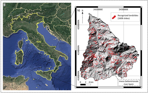
The Imera Settentrionale river basin extends for 343 km² in the northern sector of Sicily (Italy, Figure 1(a); Figure (a) of Main Map). The outcropping rocks mainly consists of carbonate, siliceous-carbonate and siliciclastic successions, which form tectonic units having imbricate geometric structures, as a consequence of the compressive phase that built up the Sicilian chain since the Oligocene (Morticelli et al., 2015). During the Late Miocene the Sicilian chain was associated with the development of wide to quite narrow syntectonic basins partly located above the growing thrust sheets (Gugliotta et al., 2013), filled with terrigenous deposits.

Figure 1. (a) Location of the Imera Settentrionale river basin; (b) Recognized active rotational/translational slides inventory map.

The area is affected by several instability phenomena (Agnesi et al., 2000; Di Maggio et al., 2017) related to the climatic conditions but also to the recurrent seismic events that occurred in the Madonie mountains area (Agnesi et al., 2005). The neotectonic activity, is also responsible for the big deep-seated gravitational slope deformation (Agnesi et al., 1997; Di Maggio et al., 2014) in the southern part of the basin. The largest part of the basin, where flysch sediments, multi-cycles sequences of alluvial clastic sediments and marine pelites outcrop, is densely marked by water erosion landforms (rills, gullies, pipes), somewhere giving rise to typical Italian ‘calanchi’ badlands systems (Buccolini et al., 2012; Cappadonia et al., 2011, 2016; Pulice et al., 2012), and landslides, which are typically of flow and slide type.

The mean annual rainfall (750 mm) and temperature values of about 16°C allow us to classify the climate of Imera Settentrionale river basin as Mediterranean type, with rainfall concentrated mainly in few of the winter semester days, while summer period is characterized by almost drought conditions.

2.2. Landslide inventory and landslide conditioning factors

Landslide recognition was carried out using high resolution (0.25 m) LIDAR (LIght Detection And Ranging) images taken in 2012 by ARTA (Assessorato Regionale al Territorio e all’Ambiente). The inventory includes 1608 rotational/translational slides that, on the whole, affect an area extended for about 26 km² (∼8% of the study area). The obtained landslides inventory (Figure 1(b)) was checked with a randomly hot spots field survey which were carried out in 2019; for each of the mapped landslide polygon the highest point along the crown (Landslide Identification Point – LIP) was extracted, which several researches (e.g. Cama et al., 2015; Lombardo et al., 2014, 2016; Rotigliano et al., 2011) highlighted as an effective diagnostic site for landslide susceptibility evaluation.

The local environmental conditions which directly influence the instability of the slopes are mainly related to morphology (slope angle, orientation slope, curvature, elevation, roughness etc.) and others predisposing characteristics (e.g. lithology, soil use, tectonic condition, landform classification). Any kind of controlling factor can be considered as a potential predictor and can be introduced into the susceptibility analysis. In this research, a set of 10 topographic predictors was derived by processing with GIS hydro-morphological tools a 8 m cell digital elevation model (DEM) obtained from a LIDAR survey in 2008 by ARTA: elevation (ELE), landform classification (LCL), steepness (STP), aspect (expressed as NORTHerness and EASTerness), plan (PLN) and profile (PRF) curvatures, topographic wetness index (TWI), terrain ruggedness index (TRI) and stream power index (SPI).

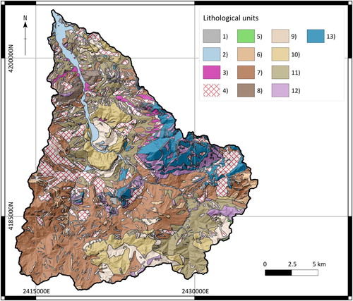
A bedrock lithology map (LITO) was prepared by grouping the different outcropping lithologies (Figure 2) in light of their expected mechanical behavior. The boundaries between the different units were verified and adapted on the basis of remote and field surveys. The Corine Land Cover 2018 (USE) was also used to classify land use of the Imera Settentrionale river basin.

Figure 2. Bedrock lithology map of the study area: (1) Anthropic deposits; (2) Alluvial deposits; (3) Alluvial fan and talus deposit; (4) Colluvium and old landslide deposits; (5) Evaporitic rocks; (6) Sandstones; (7) Flysch Numidico pelites; (8) Flysch Numidico sandstones/conglomerates; (9) ‘Terravecchia’ pelites; (10) ‘Terravecchia’ sandstones/conglomerates; (11) ‘Varicolori’ clays; (12) Calcareous and clayey marls; (13) Lithoid units.

2.3. MARS modeling

The Multivariate Adaptive Regression Splines (MARS; Friedman, 1991) stochastic method was applied to model landslide susceptibility. This method, which already proved to be suitable for landslide modeling (e.g. Conoscenti et al., 2015, 2016; Rotigliano et al., 2018, 2019; Vargas-Cuervo et al., 2019), allows us to optimize the linear regression obtained between the dependent and the independent variables.

The MARS regression function can be written as: $y=f(x)=\alpha +\sum _{i=1}^N{\beta }_i{h}_i(x)$where y is the dependent variable (the outcome) predicted by the function f(x), α is the model intercept and β_i the coefficients of the h_i basis functions, N is the number of basis functions.

In this research, the MARS models were implemented through the ‘earth’ package (Milborrow, 2019) of Rstudio software.

2.4. Pixel-based model building and validation

Each 8 m pixel was classified as stable or unstable (positive or negative cases) depending on whether or not it hosts at least one LIP and the local values of all the proxy predictors assigned. Thereby, a R dataframe was obtained and exploited to extract a suite of one-hundred balanced (positive/negative) datasets, each including the whole set of positive pixels and an equal number of randomly extracted (without replacement) subsets of negatives. Each dataset was then submitted to a balanced random partition furnishing a 75% subset for calibration and a 25% unknown subset for blind validation tests.

The model performance was analyzed in terms of a cut-off independent metric (by AUC: the Area Under the receiver operating Curve) as well as, based on an optimal cut-off (Youden, 1950), in terms of TPR and TNR (true positive and negatives rates, respectively) and related accuracy. By exploiting the availability of the one-hundred replicates, each accuracy metric was assessed also in terms of precision.

Each model was tested in predicting the validation test, first, and the whole study area, then. In fact, in evaluating the suitability of the final maps it is of great importance to verify to what extent the forced false positive generation (all the unstable status pixels are inside the calibration/validation subsets) is balanced by the performance in terms of true negative prediction.

2.5. Slope Units partitioning and scoring

By using two main criteria, 10 types of slope-unit partitioning schemes were adopted.

Firstly, two classic hydro-morphological units were obtained by means of contributing area-based procedures: in this way, by exploiting 2000 and 5000 contributing area thresholds, a 2000 half basin (2000_HB_SLU) and a 5000 half basin (5000_HB_SLU) SLU-layers were obtained.

Then, the TPI based Landform Classification (LCL; Guisan et al., 1999) SAGA tool was exploited to obtain four different LCL maps from the DEM, by changing the inner/outer radius as 100/1000, 100/2000, 500/1000 and 500/2000 meters. LCL divides and classifies the study area in geomorphological-classes considering the relative vertical position of each pixel.

By intersecting the 2000_HB_SLU and 5000_HB_SLU shapes with the four LCL maps, eight new types of slope-units were obtained (Table 1), in which each half basin unit was split into several areas having a different geomorphological classification (Figure 3).

Figure 3. Example of LCL_SLU partition (HB_SLU: 5000 + LCL: 100-2000).

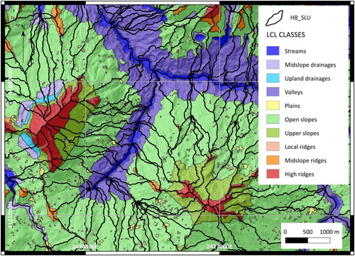
Table 1. Characteristics of the LCL_SLU partitioning scheme adopted.

Hydro-morphological units	LCL inner–outer radius	LCL_SLU
2000_HB_SLU	100–1000	211_LCL_SLU
	100–2000	212_LCL_SLU
	500–1000	251_LCL_SLU
	500–2000	252_LCL_SLU
5000_HB_SLU	100–1000	511_LCL_SLU
	100–2000	512_LCL_SLU
	500–1000	551_LCL_SLU
	500–2000	552_LCL_SLU

For each of the 10 types of obtained slope-unit layers, MEAN (average) and MSTD (mean plus one standard deviation) of the pixel-based scores were zoned for producing 10 derived prediction images. A positive (unstable) status was then assigned to the slope-units if containing at least one LIP. In this way, each slope-unit was so characterized by a predicted (derived by MEAN and MSTD scoring) and an observed status, so that Receiver Operating Curve (ROC)-plots and Confusion Matrixes, through a new Youden Index cut-off, were analyzed.

3. Results

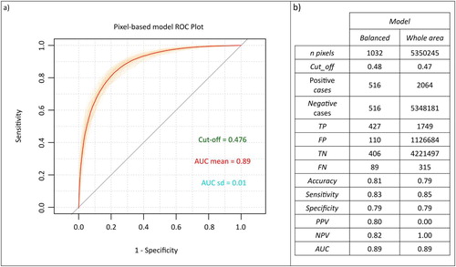
Figure 4(a), which shows the ROC-plot of the one-hundred pixel-based models, attests for excellent (Hosmer & Lemeshow, 2000) AUC mean values (0.89), associated to very low standard deviations (0.01), and a 0.48 Youden Index cut-off. A similar high performance in terms of prediction accuracy (Figure 4(b)) was also obtained from the confusion matrix both for the balanced pixel-based model and the entire area (0.79–0.81). Coherently, both specificity and sensitivity do not change from the balanced datasets (0.83) to the entire area (0.85). On the other hand, while similar (about 0.80) Positive and Negative Predicted Values (PPV and NPV) were achieved by the balanced test, very different results were obtained for the whole area (0.001 and 0.999, respectively).

Figure 4. (a) Roc plot of pixel-based model (the one-hundred replicates are plotted in orange while the averaged ROC is in red); (b) Summary of the averaged confusion matrices for the pixel-based model validations (balanced and entire area schemes).

Figure 5(a) shows a graphical resume of the most important selected predictors, by using the nsubsets criterion (Conoscenti et al., 2016; Rotigliano et al., 2019).

Figure 5. (a) Variables importance for the pixel-based model: the predictors with an overall higher than 25 are plotted in cyan while those with an overall lower than 25 are in light-cyan; (b) Binary correlation between the continuous variables: the radius of circle is proportional to the intensity of correlation (between 0 and 1) while the color is representative to the direction (yellow for positive correlation, green for negative one); the X symbol corresponds to a non-significant correlation (p-value <.01).

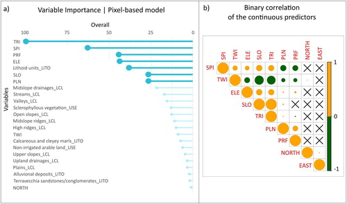
The categorical variables (LCL, LITO, USE) were disassembled into specific classes to analyze their different impact. In this way, 23 out of 45 variables have contributed to discriminate the positive to negative cases but only seven can be considered very important. TRI, SPI, PRF, ELE, SLO and PLN are the most important DEM-derived variables. Between the categorical variables, ‘lithoid units’ and ‘calcareous and clayey marls’ lithology classes, ‘non-irrigated arable land’ and ‘sclerophyllous vegetation’ land use classes and all the LCL classes played a very important role to discriminate the stable/unstable pixels.

The binary correlation between the continuous variables (Figure 5(b)) highlights a very high negative correlation between TWI and SLO, TWI and TRI whilst a positive one between SLO and TRI.

In Table 2, the MEAN- and the MSTD-derived LCL_SLU AUCs for the 10 types of slope-units are showed. The LCL_SLU AUCs perform always slightly better by using the MSTD-derived score (>0.84) rather than the MEAN-derived score (>0.82). A similar behavior is observed also for the HB_SLU models but down-shifted toward less performing results (between 0.74 and 0.78).

Table 2. Summary of the validation metrics for the 10 susceptibility models.

	Model	Number of LCL_SLU or HB_SLU	Cut_off	Positive cases	Negative cases	TP	FP	TN	FN	Accuracy	Sensitivity	Specificity	PPV	NPV	AUC
According to the MSTD	2000_HB_SLU	3519	0.45	783	2736	631	949	1787	152	0.69	0.81	0.65	0.40	0.92	0.78
	5000_HB_SLU	1544	0.46	541	1003	423	337	666	118	0.71	0.78	0.66	0.56	0.85	0.76
	211_LCL_SLU	19,165	0.35	979	18,178	914	5590	12,588	65	0.70	0.93	0.69	0.14	0.99	0.84
	212_LCL_SLU	17,443	0.35	953	16,482	899	5208	11,274	54	0.70	0.94	0.68	0.15	1.00	0.84
	251_LCL_SLU	21,398	0.36	1036	20,354	962	6484	13,870	74	0.69	0.93	0.68	0.13	0.99	0.85
	252_LCL_SLU	19,196	0.37	1045	18,143	961	5559	12,584	84	0.71	0.92	0.69	0.15	0.99	0.85
	511_LCL_SLU	14,936	0.35	763	14,160	712	4023	10,137	51	0.73	0.93	0.72	0.15	0.99	0.85
	512_LCL_SLU	13,571	0.35	736	12,823	696	3694	9129	40	0.72	0.95	0.71	0.16	1.00	0.84
	551_LCL_SLU	16,232	0.35	831	15,381	775	4640	10,741	56	0.71	0.93	0.70	0.14	0.99	0.85
	552_LCL_SLU	14,281	0.37	846	13,419	783	3786	9633	63	0.73	0.93	0.72	0.17	0.99	0.86
According to the MEAN	2000_HB_SLU	3519	0.23	783	2736	629	956	1780	154	0.68	0.80	0.65	0.40	0.92	0.77
	5000_HB_SLU	1544	0.20	541	1003	472	441	562	69	0.67	0.87	0.56	0.52	0.89	0.74
	211_LCL_SLU	19,165	0.19	979	18,178	905	5916	12,262	74	0.69	0.92	0.67	0.13	0.99	0.82
	212_LCL_SLU	17,443	0.19	933	16,482	866	5438	11,044	67	0.68	0.93	0.67	0.14	0.99	0.82
	251_LCL_SLU	21,398	0.18	1036	20,354	965	7088	13,266	71	0.67	0.93	0.65	0.12	0.99	0.83
	252_LCL_SLU	19,196	0.18	1045	18,143	975	6204	11,939	70	0.67	0.93	0.66	0.14	0.99	0.84
	511_LCL_SLU	14,936	0.18	763	14,160	704	4450	9710	59	0.70	0.92	0.69	0.14	0.99	0.82
	512_LCL_SLU	13,571	0.17	736	12,823	698	4236	8587	38	0.68	0.95	0.67	0.14	1.00	0.82
	551_LCL_SLU	16,232	0.18	831	15,381	774	5195	10,186	57	0.68	0.93	0.66	0.13	0.99	0.83
	552_LCL_SLU	14,281	0.19	846	13,419	779	4110	9309	67	0.71	0.92	0.69	0.16	0.99	0.84

The Youden Index cut-offs are lower than the pixel-based models ones, with a more marked decreasing when passing either from HB_SLU to LCL_SLU or from the MSTD- to the MEAN-derived score.

By using the MSTD-derived score, very high sensitivity values arise for all the LCL_SLU models (>0.90) together with a lower specificity (about 0.7) resulting in a less performing accuracy (about 0.7). On the contrary, the 2000_HB_SLU and the 5000_HB_SLU performances, in spite of a similar (0.81 and 0.78) sensitivity, are affected by a marked decreasing in specificity (0.65 and 0.66) resulting in a just satisfactory accuracy (about 0.7).

The principal behaviors of the HB_SLU and LCL_SLU models hold also using the MEAN-derived score but all the performances result lower than MSTD-derived score: the accuracy fall down (<0.7) due to a marked specificity decreasing (<0.7, with an extreme value equal to 0.56 for 5000_HB_SLU) while the sensitivity attains good or optimal values (between 0.80 and 0.95).

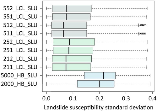
In order to explore the general coherence between pixel- and SLU-based scores for the 10 different partitioning adopted criteria, the dispersion of the pixel scores zoned into the SLUs was analyzed (Figure 6). It is worth to note that a less variability arises for HB_SLUs split by LCLs with a minimum internal radius (100 m), whilst the maximum variability arises by using the HB_SLUs (especially with the 5000_HB_SLU).

Figure 6. Boxplot of the standard deviation pixel scores zoned into the SLUs.

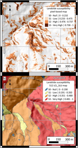
In Figure 7 a comparison between the source pixel-based and the final LCL_SLU susceptibility maps is presented for a selected representative sector. In order to objectively reclassify the susceptibility maps, three cut-off values were directly obtained by analysing the ROC-plot. A first main cut-off (m cut-off) was first identified on the ROC plot, as the probability value resulting in the maximum difference between false positive (FP) and true positive (TP) rate (Youden, 1950). The same procedure was then applied to the two semi-plots which were obtained by splitting the ROC plot using the m cut-off. In this way, the two secondary cut-off values (l and h) were identified. Exploiting the l, m and h values, the score was finally reclassified into 4 classes depending on the susceptibility interval: NULL (S0; P < l), LOW (S1; l < P < m), HIGH (S2; (S1; m < P < h)) and VERY HIGH (S3; P > h).

Figure 7. (a) Landslide susceptibility pixel-based map; (b) Landslide susceptibility LCL_SLU-based map (HB_SLU: 5000 + LCL: 100-2000).

4. Discussion and conclusions

The pixel-based model shows excellent performances both in balanced and in the entire validation area. In fact, identical excellent AUC values are obtained for the two tests and the other performance metrics reveal only a slight variation. This proves that the false positive generation in the whole area is widely balanced by the true negative successful prediction. Moreover, the one-hundred replicates demonstrate both high accuracy and precision. In light of the above, the false positive cases potentially are to be expected as future positives (in other words, future landslide initiations) rather than type I errors.

It is worth to note that the variables importance analysis shows that the LCL classes play a very important role in discriminating the landslide initiation areas. This suggests a further slope-units subdivision through the LCL classes as useful for the performant and correct identification of landslide initiation zones and, as a consequence, for developing a zonal environmental subdivision suitable for optimizing the landslide susceptibility map output.

In fact, the results confirmed that the LCL_SLU models produced homogeneous and more easy to interpret prediction images, with a predictive performance higher than HB_SLU, suffering only from a limited performance lowering with respect to the pixel-based model, almost totally dependent on type I errors (false positives); at the same time, the LCL_SLU models resulted in the highest skill in finding/predicting the unstable pixels (sensitivity). In particular, the best LCL_SLU model (HB_SLU: 5000 + LCL: 100–2000) resulted in very high performances (AUC = 0.84; sensitivity = 0.95; specificity = 0.71) and much more readable maps. Moreover, the best LCL_SLU model is characterized by a very low pixel-score variability inside each slope-unit, attesting also for a coherent and stable susceptibility zonation.

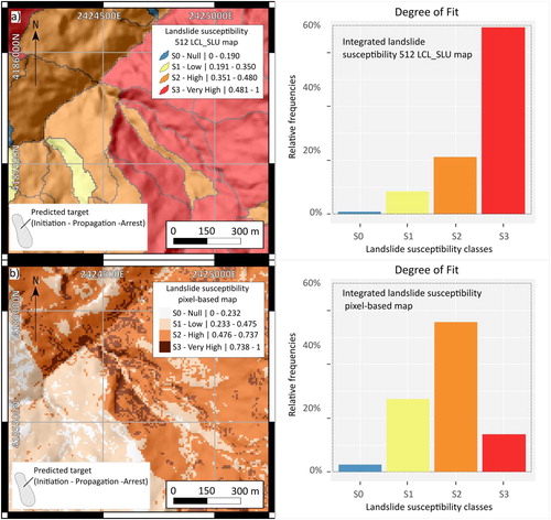
Once the best performing susceptibility map was selected, the final step was to connect the propagation stage to the landslide initiation obtained from its prediction images. To this aim, the same morphodynamic meaning of the LCL_SLU was exploited after having dissolved the LCL_SLU smaller than 20,000 m² (the 3rd quantile of the landslide frequency distribution). A degree of fit plot was then prepared to validate the new integrated susceptibility map in predicting the source landslide polygons, which actually represent the real landslide propagation/arrest areas for the calibration inventory. This plot was then compared to that obtained from a pixel-based model, which differently was calibrated using the same landslide polygons (Figure 8). The comparison between the two results attested a very more performing behavior of the LCL_SLU integrated model.

Figure 8. (a) Integrated landslide susceptibility LCL_SLU-based map (HB_SLU: 5000 + LCL: 100-2000) and whole basin degree of fit plot; (b) Landslide polygons calibrated susceptibility pixel-based map and whole basin degree of fit plot.

All the obtained results show that by integrating the classical pixel-based modeling (Figure (b) of Main Map) on the LCL_SLU mapping units (Figure (c) of Main Map), it is possible to optimize the results of the landslide susceptibility evaluation. The same LCL_SLUs allow also to involve the propagation stage into the predictive images, obtaining easy to interpret high performing integrated susceptibility maps (Figure (d) of Main Map).

Software

Google Earth Pro was employed to detect and map the landslides. GRASS GIS was utilized to partition the study area in SLU by using the r.watershed processing. Saga GIS 7.0.0 was employed to produce the LCL maps and to obtain the zonal statics analyzed. Quantum GIS 3.8.2 Zanzibar was used to clip the SLUs with the LCL maps and to print all maps displayed in this research. The modeling and the cut-off independent and dependent matrices were carried out by using the Rstudio software.

Disclosure statement

No potential conflict of interest was reported by the authors.

References

- Agnesi, V. , Camarda, M. , Conoscenti, C. , Di Maggio, C. , Serena Diliberto, I. , Madonia, P. , & Rotigliano, E. (2005). A multidisciplinary approach to the evaluation of the mechanism that triggered the Cerda landslide (Sicily, Italy). Geomorphology , 65 (1–2), 101–116. https://doi.org/10.1016/j.geomorph.2004.08.003
- Agnesi, V. , Cosentino, P. , Di Maggio, C. , Macaluso, T. , & Rotigliano, E. (1997). The great landslide at Portella Colla (Madonie, Sicily). Geografia Fisica e Dinamica Quaternaria , 19 (2), 273–280.
- Agnesi, V. , De Cristofaro, D. , Di Maggio, C. , Macaluso, T. , Madonia, G. , & Messana, V. (2000). Morphotectonic setting of the Madonie area (central northern Sicily). Memorie Della Società Geologica Italiana , 55 , 373–379.
- Amato, G. , Eisank, C. , Castro-camilo, D. , & Lombardo, L. (2019). Accounting for covariate distributions in slope-unit-based landslide susceptibility models. A case study in the alpine environment. Engineering Geology , 260 , 105237. https://doi.org/10.1016/j.enggeo.2019.105237
- Ba, Q. , Chen, Y. , Deng, S. , Yang, J. , & Li, H. (2018). A comparison of slope units and grid cells as mapping units for landslide susceptibility assessment. Earth Science Informatics , 11 (3), 373–388. https://doi.org/10.1007/s12145-018-0335-9
- Buccolini, M. , Coco, L. , Cappadonia, C. , & Rotigliano, E. (2012). Relationships between a new slope morphometric index and calanchi erosion in northern Sicily, Italy. Geomorphology , 149–150 , 41–48. https://doi.org/10.1016/j.geomorph.2012.01.012
- Cama, M. , Lombardo, L. , Conoscenti, C. , Agnesi, V. , & Rotigliano, E. (2015). Predicting storm-triggered debris flow events: Application to the 2009 Ionian Peloritan disaster (Sicily, Italy). Natural Hazards and Earth System Sciences , 15 (8), 1785–1806. https://doi.org/10.5194/nhess-15-1785-2015
- Cama, M. , Lombardo, L. , Conoscenti, C. , & Rotigliano, E. (2017). Improving transferability strategies for debris flow susceptibility assessment: Application to the Saponara and Itala catchments (Messina, Italy). Geomorphology , 288 , 52–65. https://doi.org/10.1016/j.geomorph.2017.03.025
- Cappadonia, C. , Coco, L. , Buccolini, M. , & Rotigliano, E. (2016). From slope morphometry to morphogenetic processes: An integrated approach of field survey, geographic information system morphometric analysis and statistics in Italian badlands. Land Degradation & Development , 27 (3), 851–862. https://doi.org/10.1002/ldr.2449
- Cappadonia, C. , Conoscenti, C. , & Rotigliano, E. (2011). Monitoring of erosion on two calanchi fronts-northern Sicily (Italy). Landform Analysis , 17 , 21–25.
- Carrara, A. , Cardinali, M. , Guzzetti, F. , & Reichenbach, P. (1995). Gis technology in mapping landslide hazard. In Carrara A , Guzzetti F (eds), Geographical information systems in assessing natural hazards (pp. 135–175). Kluwer, Dordrecht. https://doi.org/10.1007/978-94-015-8404-3_8
- Conoscenti, C. , Ciaccio, M. , Caraballo-Arias, N. A. , Gómez-Gutiérrez, Á , Rotigliano, E. , & Agnesi, V. (2015). Assessment of susceptibility to earth-flow landslide using logistic regression and multivariate adaptive regression splines: A case of the Belice river basin (western Sicily, Italy). Geomorphology , 242 , 49–64. https://doi.org/10.1016/j.geomorph.2014.09.020
- Conoscenti, C. , Rotigliano, E. , Cama, M. , Caraballo-Arias, N. A. , Lombardo, L. , & Agnesi, V. (2016). Exploring the effect of absence selection on landslide susceptibility models: A case study in Sicily, Italy. Geomorphology , 261 , 222–235. https://doi.org/10.1016/j.geomorph.2016.03.006
- Di Maggio, C. , Madonia, G. , & Vattano, M. (2014). Deep-seated gravitational slope deformations in western Sicily: Controlling factors, triggering mechanisms, and morphoevolutionary models. Geomorphology , 208 , 173–189. https://doi.org/10.1016/j.geomorph.2013.11.023
- Di Maggio, C. , Madonia, G. , Vattano, M. , Agnesi, V. , & Monteleone, S. (2017). Geomorphological evolution of western Sicily, Italy. Geologica Carpathica , 68 (1), 80–93. https://doi.org/10.1515/geoca-2017-0007
- Domènech, G. , Alvioli, M. , & Corominas, J. (2020). Preparing first-time slope failures hazard maps: From pixel-based to slope unit-based. Landslides , 17 (2), 249–265. https://doi.org/10.1007/s10346-019-01279-4
- Friedman, J. H. (1991). Multivariate adaptive regression splines. The Annals of Statistics , 19 (1), 1–67. https://doi.org/10.1214/aos/1176347963
- Gugliotta, C. , Agate, M. , & Sulli, A. (2013). Sedimentology and sequence stratigraphy of wedge-top clastic successions: Insights and open questions from the upper Tortonian Terravecchia formation of the Scillato basin (central-northern Sicily, Italy). Marine and Petroleum Geology , 43 , 239–259. https://doi.org/10.1016/j.marpetgeo.2013.02.004
- Guisan, A. , Weiss, S. B. , & Weiss, A. D. (1999). GLM versus CCA spatial modeling of plant species distribution author (s): Reviewed work (s): GLM versus CCA spatial modeling of plant species distribution. Plant Ecology , 143 (1), 107–122. https://doi.org/10.1023/A:1009841519580
- Guzzetti, F. , Carrara, A. , Cardinali, M. , & Reichenbach, P. (1999). Landslide hazard evaluation: A review of current techniques and their application in a multi-scale study, Central Italy. Geomorphology , 31 (1-4), 181–216. https://doi.org/10.1016/S0169-555X(99)00078-1
- Guzzetti, F. , Reichenbach, P. , Ardizzone, F. , Cardinali, M. , & Galli, M. (2006). Estimating the quality of landslide susceptibility models. Geomorphology , 81 (1-2), 166–184. https://doi.org/10.1016/j.geomorph.2006.04.007
- Hansen, A. (1984). Landslide hazard analysis. In: Brunsden D. , Prior D.B. (eds) Slope instability . Wiley, New York, pp 523–602.
- Hosmer, D.W. & Lemeshow, S. (2000). Applied logistic regression, Wiley Series in Probability and Statistics. Wiley. https://doi.org/10.1198/tech.2002.s650
- Lombardo, L. , Bachofer, F. , Cama, M. , Maerker, M. , & Rotigliano, E. (2016). Exploiting maximum entropy method and ASTER data for assessing debris flow and debris slide susceptibility for the Giampilieri catchment (north-eastern Sicily, Italy). Earth Surface Processes and Landforms , 41 (12), 1776–1789. https://doi.org/10.1002/esp.3998
- Lombardo, L. , Cama, M. , Conoscenti, C. , Märker, M. , & Rotigliano, E. (2015). Binary logistic regression versus stochastic gradient boosted decision trees in assessing landslide susceptibility for multiple-occurring landslide events: Application to the 2009 storm event in Messina (Sicily, southern Italy). Natural Hazards , 79 (3), 1621–1648. https://doi.org/10.1007/s11069-015-1915-3
- Lombardo, L. , Cama, M. , Maerker, M. , & Rotigliano, E. (2014). A test of transferability for landslides susceptibility models under extreme climatic events: Application to the Messina 2009 disaster. Natural Hazards , 74 (3), 1951–1989. https://doi.org/10.1007/s11069-014-1285-2
- Milborrow, S. (2019). Notes on the Earth Package. http://www.milbo.org/doc/earth-notes.pdf (accessed 6.6.20).
- Morticelli, M. G. , Valenti, V. , Catalano, R. , Sulli, A. , Agate, M. , Avellone, G. , Albanese, C. , Basilone, L. , & Gugliotta, C. (2015). Deep controls on foreland basin system evolution along the Sicilian fold and thrust belt. Bulletin de la Société Géologique de France , 186 (4–5), 273–290. https://doi.org/10.2113/gssgfbull.186.4-5.273
- Pulice, I. , Cappadonia, C. , Scarciglia, F. , Robustelli, G. , Conoscenti, C. , De Rose, R. , Rotigliano, E. , & Agnesi, V. (2012). Geomorphological, chemical and physical study of “calanchi” landforms in NW Sicily (southern Italy). Geomorphology , 153–154 , 219–231. https://doi.org/10.1016/j.geomorph.2012.02.026
- Reichenbach, P. , Rossi, M. , Malamud, B. D. , Mihir, M. , & Guzzetti, F. (2018). A review of statistically-based landslide susceptibility models. Earth-Science Reviews , 180 , 60–91. https://doi.org/10.1016/j.earscirev.2018.03.001
- Rotigliano, E. , Agnesi, V. , Cappadonia, C. , & Conoscenti, C. (2011). The role of the diagnostic areas in the assessment of landslide susceptibility models: A test in the sicilian chain. Natural Hazards , 58 (3), 981–999. https://doi.org/10.1007/s11069-010-9708-1
- Rotigliano, E. , Cappadonia, C. , Conoscenti, C. , Costanzo, D. , & Agnesi, V. (2012). Slope units-based flow susceptibility model: Using validation tests to select controlling factors. Natural Hazards , 61 (1), 143–153. https://doi.org/10.1007/s11069-011-9846-0
- Rotigliano, E. , Martinello, C. , Agnesi, V. , & Conoscenti, C. (2018). Evaluation of debris flow susceptibility in El Salvador (CA): A comparison between multivariate adaptive regression splines (MARS) and binary logistic regression (BLR). Hungarian Geographical Bulletin , 67 (4), 361–373. https://doi.org/10.15201/hungeobull.67.4.5
- Rotigliano, E. , Martinello, C. , Hernandéz, M. A. , Agnesi, V. , & Conoscenti, C. (2019). Predicting the landslides triggered by the 2009 96E/Ida tropical storms in the Ilopango caldera area (El Salvador, CA): Optimizing MARS-based model building and validation strategies. Environmental Earth Sciences , 78 (6). https://doi.org/10.1007/s12665-019-8214-3
- Van Den Eeckhaut, M. , Reichenbach, P. , Guzzetti, F. , Rossi, M. , & Poesen, J. (2009). Combined landslide inventory and susceptibility assessment based on different mapping units: An example from the Flemish Ardennes, Belgium. Natural Hazards and Earth System Sciences , 9 (2), 507–521. https://doi.org/10.5194/nhess-9-507-2009
- van Westen, C. J. , Rengers, N. , Terlien, M. T. J. , & Soeters, R. (1997). Prediction of the occurrence of slope instability phenomenal through GIS-based hazard zonation. Geologische Rundschau , 86 (2), 404–414. https://doi.org/10.1007/s005310050149
- Vargas-Cuervo, G. , Rotigliano, E. , & Conoscenti, C. (2019). Prediction of debris-avalanches and -flows triggered by a tropical storm by using a stochastic approach: An application to the events occurred in Mocoa (Colombia) on 1 April 2017. Geomorphology , 339 , 31–43. https://doi.org/10.1016/j.geomorph.2019.04.023
- Youden, W. J. (1950). Index for rating diagnostic tests. Cancer , 3 (1), 32–35. https://doi.org/10.1002/1097-0142(1950)3:1<32::AID-CNCR2820030106>3.0.CO;2-3