Glacial geomorphology between Lake Vänern and Lake Vättern, southern Sweden

ABSTRACT

The glacial geomorphology between the lakes Vänern and Vättern is presented on a 1:220,000 scale, LiDAR-based map covering approximately 18,000 km². Fifteen landform units have been mapped; end moraines, De Geer moraines, drumlins, crag-and-tails, hummock tracts and corridors, irregular ridges, murtoos, eskers, deltas/sandur, outwash complexes, meltwater channels, boulder bars/sheets, the Timmersdala ridge, raised shorelines, sand dunes and prominent landslide scars (the last three are post-glacial). The area includes moraines associated with the Younger Dryas cold interval and drainage deposits of the Baltic Ice Lake. Additionally, the map reveals previously undetected geomorphic features including (1) murtoos, (2) abundant traces of meltwater erosion manifested as channels and hummock corridors, (3) laterally extensive end-moraine systems (the Remmene and Kungslena ice-margin positions) and (4) the distinct lobate shape of end moraines formed above the highest shoreline. This map provides a uniform base for future use in georesources, paleo ice-sheet modelling, geologic history, and geoconservation.

KEYWORDS:

• Glacial geomorphology
• LiDAR
• Middle Swedish end-moraine zone
• Baltic Ice Lake
• deglaciation
• Younger Dryas

1. Introduction

The Quaternary geomorphology of the landscape between Vänern and Vättern (the largest and second largest lakes in Sweden, respectively) developed prior to, during and after the Younger Dryas cold interval (YD; e.g. Hughes et al., 2016; Lundqvist, 2004) and provides essential information for understanding the behaviour of the Fennoscandian Ice Sheet (FIS) deglaciation. That is, how glacier-ice moved, eroded, transported, and deposited sediment.

The diverse nature of this plateau-hill landscape has brought geoscientists to this region since at least the eighteenth century (Kalm, 1746; von Linné, 1747), followed by the first published geological maps in Sweden (Hermelin, 1767; Hisinger, 1797). However, most Quaternary research has been produced over the last century.

The most significant Quaternary features arguably include the Middle Swedish end-moraine zone (MSEMZ), which crosses the mapping area west to east, and features associated with the drainage of the Baltic Ice Lake.

Although this is one of the most thoroughly investigated Quaternary landscapes of northern Europe, a uniform and complete mapping of the Quaternary geomorphology has never been carried out. The purpose of the map is to serve societal planning needs and as a base for scientific studies in paleoglaciology and Quaternary history. The detail of the present map has been possible in large part due to the advent of ice-sheet/sector scale light detection and ranging (LiDAR) derived elevation data, which has enabled high-resolution mapping of previously undetected landforms and new details on previously well-known landforms (e.g. Johnson et al., 2015).

This map (Main Map) aims to provide a basis for all these uses, but above all to improve the understanding of the distribution and evolution of glacial landforms in the area between Lake Vänern and Lake Vättern.

1.1. Physiography of the study area

The mapped area lies in southern Sweden (Figure 1), and the large-scale physiography can be divided into three regions: (1) the flat, well-preserved sub-Cambrian peneplain, (2) the remnant Lower Phanerozoic plateau hills, and (3) the uplifted and eroded parts of the peneplain (Johansson, 2003; Lidmar-Bergström, 1999).

Figure 1. The mapped area in southern Sweden. (A) Map of the study area showing cited previous maps that include glacial geomorphology. A list of these references can be found in Table 1. (B) Locations of Figures 2–7 are shown with rectangles, ovals or points. The inset in the centre shows the map area as a red polygon in respect to Scandinavia and its surrounding.

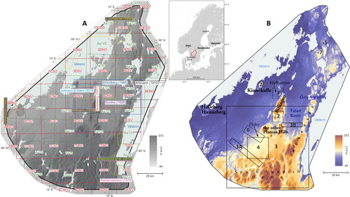
The peneplain is a low-relief feature of granite and gneissic-granite bedrock of Precambrian age that extends over large parts of Fennoscandia (Lidmar-Bergström, 1996; Lidmar-Bergström et al., 2013; Westergård, 1931). The plateau hills, for example Billingen and Kinnekulle (Figure 1(B)), are remnants of a previously extensive Paleozoic cover of sedimentary rocks (e.g. Ahlberg et al., 2013). In the southern part of the study area there is a tectonically uplifted area, corresponding to the northern slopes of the South Swedish Dome (Lidmar-Bergström, 1999; Lidmar-Bergström et al., 2017). Additionaly, there are two other uplifted crystalline bedrock features, which are of great importance when interpreting the course of events interconnected to the final drainage of the Baltic Ice Lake (see Strömberg, 1992 and referenses therein). Hökensås is a horst bordering the lake Vättern graben (Andréasson & Rodhe, 1990, 1992; Månsson, 1996), and Klyftamon at the centre of the Main Map, is marked by a dip-slip fault-line scarp (e.g. Ahlberg et al., 2013).

Superposed on this bedrock landscape lie the Quaternary landforms mapped in this study. SGUs drift-depth model (2015a; inset on the Main Map) reveal some interesting patterns. Most obvious is the thickness of sediment deposited during the YD (i.e. MSEMZ).

1.2. Previous mapping

The Quaternary surficial deposits and geomorphology in the study area have been previously mapped with different scales and coverage. A reference list of maps produced in the area is presented in Table 1 and shown in Figure 1(A). Geomorphologic features are usually included – but not uniformly documented – in the surficial-deposit mapping by the Swedish Geological Survey (SGU) (moraine ridges, drumlins, eskers, beach ridges, dunes, fluvial channels), and many prominent features (especially moraines) have been shown on national-scale maps (Lundqvist, 1961; Lundqvist & Wohlfarth, 2001; Stroeven et al., 2016). Although this region has been thoroughly studied, there is no complete coverage, concerning scale and geologic representation. Plenty of research has focused on the most prominent features or events in the region, this has perhaps led to the lack of comprehensive regional mapping. Consequently, regional mapping of the geomorphology at the resolution performed in this study on a homogeneous dataset has not been carried out before.

Table 1. List of previous maps in the area, which have included some glacial morphology. Read together with Figure 1.

Map name/description	Map tile	Reference	Published	Figure in
The SGU Surficial Deposit Database	Red tiles (e.g. 7DNV)	SGU (2016e)	SGU
Kristinehamn	Aa122	Blomberg (1903)	SGU
Furuholmarna	Aa136	Johansson (1917)	SGU
Björneborg	Aa124	Blomberg (1904a)	SGU
Otterbäcken	Aa145	Sandegren (1916)	SGU
Skagersholm	Aa128	Blomberg (1904b)	SGU
Askersund	Aa84	Erdmann (1883)	SGU
Mariestad	Aa163	Westergård (1925a)	SGU
Töreboda	Aa139	Westergård (1915)	SGU
Medevi	Aa115	Blomberg (1900)	SGU
Lidköping	Aa182	Johansson (1943)	SGU
Lugnås	Aa172	Lundqvist (1931)	SGU
Karlsborg	Aa162	Westergård (1925b)	SGU
Wenersborg	Aa40	Sidenbladh (1870)	SGU
Levene	Aa201	Mohrén (1974)	SGU
Skara	Aa116	Munthe (1900)	SGU
Sköfde	Aa121	Munthe (1905b)	SGU
Hjo	Aa132	Blomberg (1906b)	SGU
Falköping	Aa120	Munthe (1905a)	SGU
Tidaholm	Aa125	Munthe (1906)	SGU
Gällö	Aa131	Blomberg (1906a)	SGU
Wårgårda	Aa20	Fries (1866)	SGU
Sämsholm	Aa25	Fries (1867)	SGU
Gränna	Aa193	Munthe (1951)	SGU
Borås	Aa28	Stolpe (1868)	SGU
Ulricehamn	Aa21	Törnebohm (1866)	SGU
Jönköping	Aa123	Munthe (1907)	SGU
Karta öfver randbildningar	Ahlmann (1910)	Ahlmann (1910)		Tafl. 1
Die fenno-skandischen Endmoränenzüge	Ahlmann (1916)	Ahlmann (1916)		Tafel 1
Glacialgeologisk karta över Billingen-Falbygden	Munthe (1928)	Munthe (1928)		Tavl. 1
Surficial deposits in Värmlands län	Lundqvist (1958)	Lundqvist (1958)	SGU
Map of the inland-ice deglaciation	full cover	Lundqvist (1961)	SGU
Meltwater channels at N Billingen	Strömberg (1977)	Strömberg (1977)		Fig. 1
Geomorphological map of the S Vättern area	Waldemarson (1979)	Waldemarson (1979)		Fig. 6
Ice-marginal depositions in N Bohuslän and S Dalsland	Johansson (1982)	Johansson (1982)		PL. 1
The Billingen – Lake Vättern area	Strömberg (1985)	Strömberg (1985)		Fig. 1
National Atlas of Sweden, Superficial shapes	full cover	Hilldén (2003)		p. 101
National Atlas of Sweden, Västra Götaland	full cover	Lundqvist (2009)		p. 134
End-moraine ridges west of Billingen	Johnson and Ståhl (2010)	Johnson and Ståhl (2010)		Fig. 1
Crag-and-tails of the E Vättern ice lobe	Greenwood et al. (2015)	Greenwood et al. (2015)		Fig.7
Eskers and ice-marginal positions	full cover	Stroeven et al. (2016)		Fig. 5 & 11

1.3. A brief description of the deglacial history

After reaching the late glacial maximum position in Germany, the FIS began to melt back. The ice margin reached the southwestern parts of the mapping area around 13,600 cal yr BP during the Bølling warm period, during the YD the ice margin readvanced or experienced stillstands, and it finally left the northern tip of the map at 11,100 cal yr BP during the early Holocene (Hughes et al., 2016; Påsse & Daniels, 2015; Stroeven et al., 2016).

These events left the position of the former ice margin clearly marked with a series of end moraines, including those formed during the YD. The ice margin retreated northwards in a marine environment west and north of Billingen, and several glacial lakes including Tidan, Vättern and the Baltic Ice Lake, were formed east of Billingen (Figure 1(B); Påsse & Pile, 2016), marked by paleo shorelines and lake sediment. Approximately 65% of the study area experienced a marine or lacustrine deglaciation due to isostatic depression (SGU, 2015c). The Baltic Ice Lake existed east of Billingen until the ice margin reached Billingens northern tip causing the water level in the Baltic to reach sea level (Björck, 1995; Jakobsson et al., 2007; Strömberg, 1992).

Shorter-term events were also important, especially north of the YD moraines, where the abundant De Geer moraines witnesses of seasonal response rather than being related to longer-term events (De Geer, 1889; Hoppe, 1959).

2. Methods

The landforms were mapped using the Swedish national elevation model, a 2 m resolution digital elevation model (DEM) derived from airborne LiDAR (Lantmäteriet, 2016). Alternating use of five hillshades, with illumination azimuths of 270°, 315°, 0°, 45°, and 90°, slope and aspect models enabled unbiased mapping of landforms. Scales studied were approximately 1:8000 during the elementary mapping (single features) except for larger scale features which were mapped at 1:25,000 and 1:50,000. The map display scale is 1:220,000.

To further support landform interpretations, SGU geological maps and databases were used including the Surficial Deposit Database (SGU, 2016e) throughout, as well as Drift Depth (SGU, 2015a), Bedrock (SGU, 2016a), Glacial Striations (SGU, 2015b), Landslides and Ravines (SGU, 2016c) and Geophysical data such as Magnetic Field (SGU, 2016d) and Gamma Radiation (SGU, 2016b). Landforms with uncertain origin were inspected on 0.5 m resolution orthophotos (Lantmäteriet, 2015) and by Google StreetView and/or Microsoft Bird’s Eye (SIGGIS, 2016) where such information was available for ‘desktop fieldwork’. Paleogeographic shoreline displacement maps by Påsse and Daniels (2015) assisted the mapping. The paleo-water depth map (inset on the Main Map) was modelled from data in the SGU Highest Coastline database (SGU, 2015c) using ArcGIS tools (ESRI, 2018); raster calculation (Minus) and interpolation (NaturalNeighbor) from points extracted (FeatureVerticesToPoints) from the generated SGU polygons. It shows the maximum water depth reached over time at a given location.

The mapped geomorphology has been selectively verified with field controls during 2013, 2015, 2016 and 2017 with a main focus to assess ambiguous landforms. Mapping was cross-checked with previous investigations (Figure 1(A) and Table 1). Some landforms, for example in the units glacial lineations and shorelines, have deliberately been left out for the sake of map clarity.

3. Results – mapped landforms

The new glacial geomorphological map of the study area presents a more detailed inventory of landforms than previous studies. There are more individual landforms as well as more types of landforms presented here than recognised before. Although the map is focused on glacial geomorphology, three units – shorelines, sand dunes and landslide scarps – are postglacial. Table 2 presents the individual count of the over 30,000 features mapped. The mapped units are described in the following section. Locations of the presented figures are shown in Figure 1(B).

Table 2. More than 30,000 features where mapped in this study. The individual count and sum of landforms are displayed, as well as the type of map feature.

Landform unit	Features (n)	Mapped as (feat. type)
Landslide scars	5	polyline
Sand Dunes	1085	polygon
Shorelines	1294	polyline
Boulder Bar/sheets	61	polygon
Timmersdala ridge	1	polygon
Outwash complexes	304	polygon
Meltwater channels	1076	polyline
Deltas and sandurs	652	polygon
Crevasse squeeze ridges	132	polygon
End moraines	1397	polygon
De Geer moraines	11,665	polygon
Irregular ridges	2703	polyline
Eskers	2334	polygon
Hummock tracts	380	polygon
Corridor margins	225	polyline
Murtoo fields	47	polygon
Ribbed-moraine tracts	8	polygon
Drumlins	6505	polyline
Crag and tails	2900	polyline
Total	32,786

3.1. Glacial lineations

Glacial lineations include erosional and constructional, elongated to oval landforms composed of sediment that record the ice-flow orientation. The lineations are divided into ‘crag-and-tails’ and ‘drumlins’. Glacial lineations are presented as a symbol indicating the orientation of the mapped feature. Both types appear over the entire area; below and above the highest shoreline, in smooth streamlined areas, in areas of high and low relief, and even in hummock tracts.

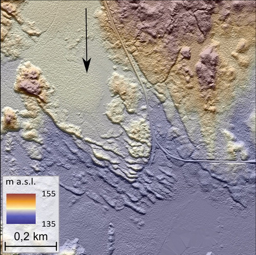
A visible obstacle such as bedrock or other obstruction at the up-ice end of the landform is the requirement for a crag-and-tail. Particularly striking are the long-streamlined tails that emerge out from the down-ice edges of several of the plateau hills (Figure 2). The median length of crag and tails in the region is 297 m (P50), with the longest features being more than 600 m (P90: 642 m).

Figure 2. Drumlins that extend from the lee side of the plateau hills are special features on the map (one example is pointed out with an arrow). The flat surfaces of the plateau hills are capped with dolerite. The oval inset shows highly elongate drumlins on top of Kinnekulle. Also note ‘pre-crag’ drumlins on the up-ice side of Kinnekulle (arrows). The extent of the figure is displayed in Figure 1(B).

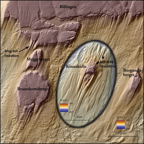
All other glacial lineations are mapped as drumlins. Drumlins with the classical egg-half shape occur as a swarm in a topographic low northeast of Billingen. At the up-ice side of Billingen and Kinnekulle, pre-crag drumlins are observed (inset in Figure 2). The median length of drumlins in the region is 312 m (P50), with the longest features being more than 700 m (P90: 734 m).

Previous mapping of drumlins (SGU, 2016e) only shows a fraction (570) of the 6500 that are presented here. Glacial striations (SGU, 2015b; inset on the Main Map) correspond well to the big picture presented by lineations. However, the mapped lineations provide more details, especially at the map centre and eastern parts where striations are rare.

3.2. Hummock tracts and corridors

We define hummocks as mounds and ridges occurring in a disorganised to semi-ordered manner. Hummock tracts are mapped where the landscape is composed of predominantly hummocks. The hummock tracts are commonly elongate and occur subparallel to ice-flow direction (Figure 3). The majority of hummock tracts occur above the highest shoreline. Within the hummock tracts, the hummocks often occur clustered in depressions. Hummocks that are more linear and elongated are mapped as ‘irregular ridges within hummock tracts’.

Figure 3. Map showing topography, water level at the highest coastline (a time-transgressive surface), hummock tracts, hummock-corridor margins, eskers, and end moraines in the southern part of the map area. Note that end moraines are lobate where they were formed above the highest shoreline, but their shape is much straighter where submerged. The highest paleocoastline is at c. 115 m above the present sea level in the southwestern part of the figure, c. 120 m a.s.l. in the northwestern parts, and c. 145 m a.s.l. inside the glacial Lake Tidan (see also Figure 1(B)). Insets show end moraines that mark the (A) Kungslena and (B) Remmene ice-margin positions. Black arrows point at the ends of the most prominent sections. The mapped end moraines are also coloured with a transparent blue colour. The extent of the figures is displayed in Figure 1(B).

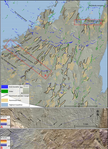
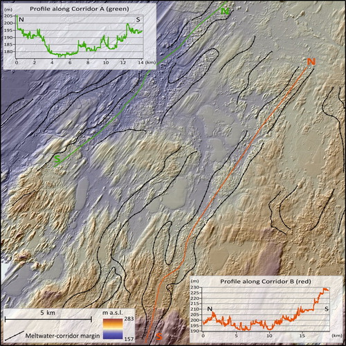
Hummock corridors are mapped only where an elongate hummock tract has sharply defined boundaries to the surrounding, smooth till plain. These can be assumed to be most clearly developed in areas with extensive till cover. Consequently, this reflect the distribution of corridors within the mapped area. The longitudinal axes of the corridors can occur on slopes dipping up-slope or down-slope with respect to the former ice-flow direction (Figure 4). Many of the hummock tracts exist as corridors, and they occur in a radial pattern that is roughly parallel to regional ice-flow direction (Figures 3 and 4). Moreover, hummock corridors have been suggested to reflect former large-scale subglacial meltwater flow beneath ice sheets (Peterson & Johnson, 2018; Sharpe et al., 2017; Utting et al., 2009). Although glacial hummocks have been commonly associated with dead-ice processes, we consider the hummock tracts to be the product of multiple processes including dead-ice melting (Johnson & Clayton, 2003; Peterson & Johnson, 2018).

Figure 4. Hummock corridors stand in stark contrast here to the surrounding streamlined drumlin topography. Inset graphs show the longitudinal profiles of two hummock corridors. The extent of the figure is displayed in Figure 1(B).

3.3. Ribbed moraines

Ribbed moraines are curved or anastomosing ridges, oriented normal to ice flow. Obvious ribbed moraine in the sense of the Swedish Åsnen (Möller, 1987) or Rogen (Lundqvist, 1969b) types does not occur. There are however some tracts with ribbed-ridge patterns (c.f. Dunlop & Clark, 2006) and in a few locations, they have a distinct appearance.

3.4. Murtoos

Murtoos (Ojala et al., 2019) occur in the study area (Figure 5). These landforms have a V-shape with apices oriented down ice. Occasionally, the V is one legged, i.e. only one scarp, and appear somewhat ragged. They are asymmetric with a gentle stoss side and steep lee-side slope. Murtoos occur in fields and are in places located at the down-ice side of hills.

Figure 5. An example of murtoos mapped in the study area. Black arrow displays former ice-flow direction, based on glacial lineations. The murtoos are composed entirely of surficial, glacial sediment. The extent of the figures is displayed in Figure 1(B).

3.5. Eskers

Eskers generally occur along valley floors, but rarely in the centre, preferring to form on either or both sides of the larger valleys. Eskers are not present at the surface in the western part of the map. The reason for this is not obvious but we suggest that abundant marine clay sediment could have covered them. Although it is most obvious for eskers, this is true also for other glacial landforms; such as drumlins and moraines. Spacing between eskers is commonly between 5 and 20 km with an average of 13 km, north of the YD moraines. South of the YD moraines, on the northern slopes of the south Swedish dome, the esker spacing is 2–7 km. The eskers are generally both wider and higher in the marine-terminating area (north of the YD), which, together with a higher retreat rate (e.g. Hughes et al., 2016), would indicate that larger channels instead of increasing numbers were formed during ice-margin retreat.

3.6. De Geer moraines

De Geer moraines are low-relief, parallel to subparallel, distinct and sharp crested ridges that occur in swarms. They are interpreted as subaquatic, ice-marginal ridges, oriented normal to ice flow (De Geer, 1940). Ojala et al. (2015) show a strong correlation of ridge spacing and proglacial water depth implying ice-margin retreat was faster in deeper water. Our analysis shows that the ridges were formed in water depths between 0 and 110 m, however, without any clear connection between appearance and depth.

Many De Geer moraines are likely ice-marginal annual moraines, but others that are more irregular may have had a more complicated genesis, including squeezing in near-margin crevasses (Bouvier et al., 2015; Ojala et al., 2015; Strömberg, 1965). De Geer moraines are often well developed and equally spaced, which is commonly interpreted as due to annual formation (Bouvier et al., 2015; Lundqvist, 1969a).

In general, the De Geer moraines are better preserved in low relief areas but can appear in more rugged bedrock dominated areas as well. In few places, for example along Hökensås, Kinnekulle and just east of the Remmene’ IMP, De Geer moraines are mapped above the highest shoreline of the sea, interpreted to have formed in proglacial lakes.

3.7. End moraines

Individual end moraines in the area have a size range between c. 20–700 m in width and between 100 m to 15 km in length, and the majority are widely traceable laterally as ice-margin positions (IMP), including the well-known Trollhättan and Levene moraines and the MSEMZ.

The MSEMZ is a swath of end moraines that were formed by an oscillating, retreating ice-margin (Johnson & Ståhl, 2010; Johnson et al., 2019; Strömberg, 1992, 1994) during the YD (e.g. Johnson & Ståhl, 2010; Lundqvist & Wohlfarth, 2001; Stroeven et al., 2016). The MSEMZ is shaded on the Main Map. The MSEMZ are broadly chrono-correlated to the Norwegian Ra-Ås-Ski moraines (Andersen et al., 1995) and the Finnish Salpausselkä moraines (De Geer, 1917b, 1917a; Donner, 2010).

South of the MSEMZ lie end moraines that mark the Levene IMP and the Trollhättan IMP (Berglund, 1979; Lundqvist & Wohlfarth, 2001; Stroeven et al., 2016). However, an additional band of end-moraine segments representing an IMP located between the Trollhättan- and Levene IMPs can be followed continuously for c. 43 km, and it seems this position has not been reported before, except for an eastern portion of one, 8 km long, mapped by Stroeven et al. (2016). This IMP is here referred to as the ‘Remmene moraine’ (Figure 3(A)).

In the centre of the Tidan basin, there are end moraines that form a distinct IMP south of the MSEMZ for 20 km, here referred to as the ‘Kungslena moraine’ (Figure 3(B)). The western segment (3 km) is mapped in Stroeven et al. (2016). On the eastern side of Billingen and south of the multiple MSEMZ ridges at Skövde is an end moraine that often is included in the MSEMZ (e.g. Berglund, 1979; Lundqvist & Wohlfarth, 2001) and correlated to the Skara and Norra Lundby moraines west of Billingen (Munthe, 1928). Here, we call it the ‘Värsås moraine’ but do not include it in the MSEMZ as done previously (e.g. Berglund, 1979; Lundqvist & Wohlfarth, 2001) because it lies further south (8 km) of the otherwise closely spaced MSEMZ moraines at Skövde.

3.8. Crevasse-squeeze ridges

These are ridges that largely reflect the crevasse pattern of the glacier and are associated to surging glaciers in soft-sediment environments; generates an extending ice tension at the glacier snout (Sharp, 1985; Evans & Rea, 1999).

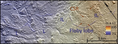
A cluster of ridges located inside a small lobate moraine, the Floby lobe (Figure 6), south of Billingen are interpreted as crevasse-squeeze ridges, based on their radial pattern that merges into a transverse one c. 2 km inside the margin and its soft sediment nature.

Figure 6. The terrestrial-terminating ice-lobe landforms at Floby. Inside the lobate shape there are ‘crevasse-squeeze ridges’ (CSR) highlighted by red arrows. Another couple of lobes (L) and interlobate areas (IL) are marked. Note the extensive traces of flowing meltwater; channels and corridors. The extent of the figure is displayed in Figure 1(B).

3.9. Deltas and sandur

This landform unit includes plateaus and other flat-topped accumulations of glaciofluvial sediments that often have a delta shape. They record the water level at the time of formation.

Some of the delta and sandur surfaces are graded to sea level or to water levels in the Baltic basin, but some represent more local ice-dammed lakes. This is common along the southwest side of Vättern, where the Vättern ice lobe recurrently dammed water at various levels during deglaciation (Greenwood et al., 2015; Waldemarson, 1986) and in the Tidan basin where numerous lake levels have been identified (Påsse & Pile, 2016).

3.10. Outwash complexes

Large accumulations of glaciofluvial outwash where no clear delta or sandur surface is visible in the data set have been mapped as ‘outwash complexes’. Pits from melting dead ice are common. The most prominent outwash complexes are the extensive areas of outwash around Skövde and west of Billingen; an area known as Valle Härad.

3.11. Meltwater channels

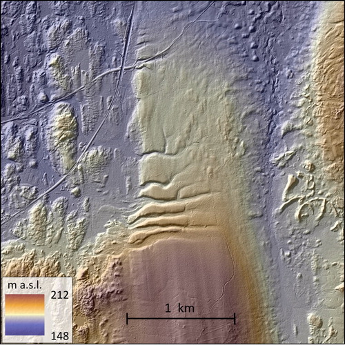
Channels incised into surficial deposits or sedimentary bedrock by the erosional forces of subglacial or proglacial meltwater are included in this unit. Proglacial meltwater can be forced along or close to the ice margin and could therefore record the ice-margin position (Greenwood et al., 2007; Mannerfelt, 1949), for example, as channels cutting into drumlins (Figure 7). Channels related to Late-glacial to early-Holocene meltwater activity are hard to distinguish from recent drainage channels, however it is reasonable to assume that Holocene channels follow similar pathways as the ones eroded by glacial meltwater.

Figure 7. Ice-marginal meltwater channels cut into a drumlin. These channels formed from the drainage of an ice-dammed lake to the east: as the ice retreated, it opened lower passages to the west. The location of the figure is displayed in Figure 1(B).

3.12. Boulder bars/sheets and the Timmersdala ridge

These two map units include landforms associated with the final drainage of the Baltic Ice Lake. Most of these are located on Klyftamon and are special features on the Main Map (Figure 8). These deposits have been reported to be composed of massive, coarse, poorly sorted and loose sediment (Figure 8; Johansson, 1926; Lundqvist, 1931; Öhrling et al., 2014; Påsse & Pile, 2016; Strömberg, 1992). The morphology displays elongated landforms laid down in the direction of drainage flow occurring at topographic locations where the flow would have lost competence; all boulder bars are located promptly in the lee of protruding bedrock. The boulder sheets are located also on lee sides but foremost where water depth would have increased abruptly.

Figure 8. Klyftamon, the Lången valley, Timmersdala ridge, and the northern tip of Billingen. Timmersdala ridge and the boulder bars were formed during the final drainage of the Baltic Ice Lake. The extent of the figure is displayed in Figure 1(B). Lower picture shows an exposure of drainage sediment at Stora Mon. Drainage-flow direction right to left.

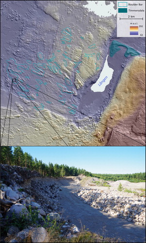
The Timmersdala ridge formed during the drainage, but has a unique morphology and sedimentology (Påsse & Pile, 2016) and deserves a separate map unit due to its unique character and well-debated genesis (Johansson, 1926, 1937; Lundqvist, 1931; Påsse & Pile, 2016; Strömberg, 1992). The landform is a large ridge transverse to ice flow, crossing a 2.5 km wide depression. The Timmersdala ridge has been considered both an end-moraine (Ramsay, 1924; Lundqvist et al., 1931) and a drainage deposit (Gavelin, 1926; Johansson, 1926, 1937). Påsse and Pile (2016) show that the ridge is generally built up from east to west indicating a progradation of the form during construction. Boulders are common on the ridge surface but rare in exposures. These characteristics led Påsse and Pile (2016) to interpret the ridge as a drainage feature formed in a subglacial tunnel.

The drainage event and the deposits formed during this event are discussed in depth in a forthcoming manuscript (Öhrling et al., 2020).

3.13. Shorelines

Paleo shorelines were formed by sediment erosion (forming a wave-cut cliff), deposition (forming a beach ridge or beach plain), or both. Many of the mapped shorelines represent the highest shoreline of the sea (99–162 m a.s.l. in the study area), but some are from ice-dammed lakes, including the Baltic Ice Lake and glacial Lake Tidan. At several locations along Hökensås there are delta surfaces or shorelines high above the highest shoreline. The highest mapped shoreline, from this mapping, is situated in the Hökensås area at 268 m a.s.l. Furthermore, the mapping shows shorelines at 150 m a.s.l. on the north-northeastern slopes of Billingen and at 125 m a.s.l. on the northwestern side. This supports the prevalent view of the water level in the BIL before and after the drainage (e.g. Lundqvist, 1921, 1931).

3.14. Sand dunes

The sand dunes mapped are directly associated with lake beds, glaciofluvial deltas or superimposed on eskers and raised beach ridges where sand would have been plentiful. The largest fields are found at former low-relief beaches, often in connection to eskers or outwash complexes.

The mapped sand dunes exhibit a wide variety of dune morphologies, including barchan, straight crested, parabolic, irregular, or mounds. The vast majority of the dunes occur in five dune fields. The three largest fields are located at c. 80–100 m a.s.l. in the southwestern and central parts of the Main Map.

3.15. Prominent landslide scars

Knowledge of landslide locations can be used for general assessment of landslide susceptibility and ground stability. Landslide scars were identified by scars and slide masses. We only include four significant landslides for two reasons. First, these are interpreted as to have occurred in early Holocene due to land uplift; the Råda landslide (Smith et al., 2014, 2017), the Mariedal landslide (S. Johansson, 1937; Smith et al., 2017), the Lerdala landslide (Smith et al., 2017) and the Lidetorp landslide. Second, inclusion of younger scars would affect map-reading clarity as well as not being directly connected to the deglacial history.

4. Discussion

The Late glacial and early Holocene geomorphology between Sweden’s two biggest lakes Vänern and Vättern is presented in a map with scale 1:220,000.

The landform record within this map (Main Map) provides more detail and provides a basis for future ice-margin and ice-dynamic reconstructions.

In this discussion we aim to draw attention to features and landforms characteristics that have emerged specifically from this mapping.

4.1. Lobate end moraines vs. straight end moraines and new end moraines

Significantly, there are two new, laterally continuous, ice-marginal lines that we have mapped. We refer to them here as the Remmene and Kungslena IMPs (Figure 3). The Trollhättan and Levene IMPs have been recognised for over 80 years (see Berglund, 1979), and they occur as nearly straight lines where the ice margin was in the sea.

Most striking is that all of these ice-margin positions are marked by lobate end moraines where they were formed above the highest shoreline (Figure 3). Stroeven et al. (2016) mapped end moraines, and the lobate shape can be discerned in their Figure 11. But our Main Map shows the distinct lobate form in these moraines as well as in the Remmene end moraine.

There are about 25 such moraine lobes across the upland south of Billingen. The lobes tend to be parallel to each other when comparing adjacent IMPs. The lobation does not appear to be related to the bedrock topography along the actual ice-margin position but seems to reflect the topography up-ice of these features, for example the plateau hills. Additionally, the lobe positions seem to be related to the subglacial drainage system indicated by the hummock corridors (see 4.2). The crevasse-squeeze ridges inside the Floby lobe (Figure 6) imply a surging ice lobe. The mechanism regarding meltwater and lobes is further discussed in Section 4.2. The straight-line orientation of these IMPs to the west is suggested to reflect the calving margin of the ice and the evenness of the subcambrian peneplain, which produced a uniform water depth.

4.2. Distribution of Hummock tracts and hummock corridors

Hummock tracts reveal a pattern of radial corridors (Figure 3), roughly parallel to the ice-flow direction.

Some hummock corridors are cut into the streamlined uplands and have a negative transverse profile, these can be interpreted as tunnel valleys (Ussing, 1903; Wright, 1973), whereas others occur as positive forms and are interpreted as subglacial, glacifluvial meltwater corridors, draped on pre-existing lineations (Brennand & Sharpe, 1993; Peterson & Johnson, 2018; St-Onge, 1984). In both cases, the corridors post-date the subglacial streamlining.

The hummock corridors in the southern supra-marine part of the landscape have an interesting pattern where found with the lobate end moraines. The corridors are often truncated along the lines of these lobate end moraines (Figure 3), suggesting that they could have been erased or covered by deposits from advancing ice lobes. The corridors are most commonly associated with the interlobate areas. This indicates that there could be a relationship between the corridors and the spatial distribution of the lobes. The concentration of meltwater into the interlobate areas could increase the effective pressure and consequently increase friction at the ice-bed interface close to the corridor. Contrary, in the lobate areas effective pressure is lower, inhibiting friction leading to increased ice-flow velocity (e.g. Boulton et al., 2009).

The geomorphic expression is insufficient to differentiate between hummocks formed from the melting solely of dead-ice and those associated with subglacial meltwater. Although many of the hummock tracts appear as hummock corridors, many hummocky areas are likely also the result of dead-ice melting. Nonetheless, De Geer moraines or eskers in places superpose hummocks, supporting a subglacial genesis for some of the hummock tracts. Moreover, the longitudinally undulating centrelines of corridors, adverse to flow direction in places, indicates evidence of a high hydrological pressure.

5. Conclusions

This map (Main Map) presents an inventory of Late glacial-early Holocene landforms between Vänern and Vättern based on LiDAR DEMs.

We regard as stand-out observations the following:

• A distinct morphological change in the end moraines of several ice-margin positions from straight, where the ice margin lay in the sea, to lobate where the ice margin was above the marine limit.

• Widespread radial hummock corridors likely formed in relation to subglacial meltwater activity.

• Murtoos occur within the mapped area.

Over 30,000 individual landforms were mapped, which presumably will help bring the understanding of the FIS deglaciation forward. For example: Mapped shore levels increase the precision of the IMP before, during, and after the drainage of the Baltic Ice Lake; Shore levels, glaciofluvial landforms, and moraines enables an improved model of the interaction between the large paleo glacial lakes; Imprints from extensive glacial meltwater enforce the re-interpretation of several areas of hummocky terrain. We hope this map will encourage formulation of new questions, bring clues to old ones, and promote geodiversity actions in the area.

Software and computer equipment

The mapping was carried out using ESRI ArcGIS® 10.2 and 10.3. The final layout of the Main Map was produced with Adobe Illustrator® 24.0.2. All mapping was conducted on a Wacom® CINTIQ® 27” digital drawing board.

Acknowledgements

We thank the Swedish Geological Survey for funding. The main author thanks Oskar Isaksson Dreyer for the collaboration with the drainage sediments on Klyftamon. We thank Jan Lundqvist, Mats Olvmo, and Jakob Heyman for comments on the manuscript and the map. Further, we thank the reviewers Sarah Greenwood and Frances Butcher for thoughtful comments that greatly improved the manuscript, and also the cartographic reviewer Nicholas Scarle. Finally, we are grateful for the help from the associate editor Paul Dunlop.

Disclosure statement

No potential conflict of interest was reported by the author(s).

References

- Ahlberg, P., Calner, M., Lehnert, O., & Wickström, L. (2013). Regional geology of the Västergötland province, Sweden. In: M. Calner, P. Ahlberg, O. Lehnert, and M. Erlström (Eds.). The Lower Palaeozoic of southern Sweden and the Oslo Region, Norway. Field Guide for the 3rd Annual Meeting of the IGCP project 591, Uppsala, Sveriges geologiska undersökning Rapporter och meddelanden 133, pp. 37–58. Retrieved May 2017, from http://resource.sgu.se/produkter/rm/rm133-rapport.pdf
- Ahlmann, H. W. (1910). Studier öfver de medelsvenska ändmoränerna. Arkiv För Kemi, Mineralogi Och Geologi, 3(29), 1–15.
- Ahlmann, H. W. (1916). Die fenno-skandischen Endmoränenzüge auf und neben dem Billingen in Vester-Götland. Zeitschrift Gletcherk Berlin.
- Andersen, B. G., Mangerud, J., Sørensen, R., Reite, A., Sveian, H., Thoresen, M., & Bergstrøm, B. (1995). Younger Dryas ice-marginal deposits in Norway. Quaternary International, 28, 147–169. https://doi.org/10.1016/1040-6182(95)00037-J
- Andréasson, P.-G., & Rodhe, A. (1990). Geology of the Protogine Zone south of Lake Vättern, southern Sweden: A reinterpretation: Geologiska Foereningan i Stockholm. Foerhandlingar, 112, 107–125. https://doi.org/10.1080/11035899009453168
- Andréasson, P.-G., & Rodhe, A. (1992). The protogine zone. Geology and mobility during the last 1.5 Ga. SKB report.
- Berglund, B. E. (1979). The deglaciation of southern Sweden 13,500-10,000 B.P. Boreas, 8(2), 89–117. https://doi.org/10.1111/j.1502-3885.1979.tb00789.x
- Björck, S. (1995). A Review of the history of the Baltic Sea. Quaternary International, 27, 19–40. https://doi.org/10.1016/1040-6182(94)00057-C
- Blomberg, A. (1900). Geologiska kartbladet Medevi. Sveriges Geologiska Undersökning, Serie Aa(115).
- Blomberg, A. (1903). Geologiska kartbladet Kristinehamn. Sveriges Geologiska Undersökning, Serie Aa(122).
- Blomberg, A. (1904a). Geologiska karbladet Björneborg. Sveriges Geologiska Undersökning, Serie Aa(124).
- Blomberg, A. (1904b). Geologiska kartbladet Skagersholm. Sveriges Geologiska Undersökning, Serie Aa(128).
- Blomberg, A. (1906a). Geologiska kartbladet Gällö. Sveriges Geologiska Undersökning, Serie Aa(131).
- Blomberg, A. (1906b). Geologiska kartbladet Hjo. Sveriges Geologiska Undersökning, Serie Aa(132).
- Boulton, G. S., Hagdorn, M., Maillot, P. B., & Zatsepin, S. (2009). Drainage beneath ice sheets: Groundwater–channel coupling, and the origin of esker systems from former ice sheets. Quaternary Science Reviews, 28(7-8), 621–638. https://doi.org/10.1016/j.quascirev.2008.05.009
- Bouvier, V., Johnson, M. D., & Påsse, T. (2015). Distribution, genesis and annual-origin of De Geer moraines in Sweden: Insights revealed by LiDAR. GFF, 137(4), 319–333. https://doi.org/10.1080/11035897.2015.1089933
- Brennand, T. A., & Sharpe, D. R. (1993). Ice-sheet dynamics and subglacial meltwater regime inferred from form and sedimentology of glaciofluvial systems: Victoria Island, District of Franklin, Northwest Territories. Canadian Journal of Earth Sciences, 30(5), 928–944. https://doi.org/10.1139/e93-078
- De Geer, G. (1889). Ändmoräner i trakten mellan Sånga och Sundbyberg. Geologiska föreningens i Stockholms förhandlingar, 11(7), 395–397. https://doi.org/10.1080/11035898909445835
- De Geer, G. (1917a). Fjärrkonnektioner längs de finiglaciala gränsmoränerna. Geologiska Föreningen i Stockholm Förhandlingar, 39(2), 185–187. https://doi.org/10.1080/11035891709444419
- De Geer, G. (1917b). Om fjärrkonnektioner längs de gotiglaciala gränsmoränerna i Scandodania och Nordamerika. Geologiska Föreningens i Stockholm Förhandlingar, 39, 18–22.
- De Geer, G. (1940). Geochronologia suecica principles. Kungliga svenska vetenskapsakademiens handlingar, 3(18), 367.
- Donner, J. (2010). The Younger Dryas age of the Salpausselkä moraines in Finland. Bulletin of the Geological Society of Finland. Retrieved March 2017, from http://www.geologinenseura.fi/bulletin/Volume82/Donner_2010.pdf
- Dunlop, P., & Clark, C. D. (2006). The morphological characteristics of ribbed moraine. Quaternary Science Reviews, 25(13-14), 1668–1691. https://doi.org/10.1016/j.quascirev.2006.01.002
- Erdmann, E. (1883). Geologiska kartbladet Askersund. Sveriges Geologiska Undersökning, Serie Aa(84).
- ESRI. (2018). ArcGIS.
- Evans, D. J. A., & Rea, B. R. (1999). Geomorphology and sedimentology of surging glaciers: A land-systems approach. Annals of Glaciology, 28, 75–82. https://doi.org/10.3189/172756499781821823
- Fries, J. O. (1866). Geologiska karbladet Wårgårda. Sveriges Geologiska Undersökning, Serie Aa(20).
- Fries, J. O. (1867). Geologiska kartbladet Sämsholm. Sveriges Geologiska Undersökning, Serie Aa(25).
- Gavelin, A. (1926). Comments on a lecture. Geologiska Föreningen i Stockholm Förhandlingar, 48.
- Greenwood, S. L., Clark, C. D., & Hughes, A. L. C. (2007). Formalising an inversion methodology for reconstructing ice-sheet retreat patterns from meltwater channels: Application to the British Ice Sheet. Journal of Quaternary Science, 22(6), 637–645. https://doi.org/10.1002/jqs.1083
- Greenwood, S. L., O’Regan, M., Swärd, H., Flodén, T., Ananyev, R., Chernykh, D., & Jakobsson, M. (2015). Multiple re-advances of a Lake Vättern outlet glacier during Fennoscandian Ice Sheet retreat, south-central Sweden. Boreas, 44(4), 619–637. https://doi.org/10.1111/bor.12132
- Hermelin, S. G. (1767). Profil af Kinnekulle ifrån Öster till Wäster (map). Rön och försök, hörande till mineral-historien öfver Skaraborgs län i Wästergötland.
- Hilldén, A. (2003). Superficial shapes. In Frizell & Werner (Ed), Västra Götaland - Sveriges nationalatlas.
- Hisinger, W. (1797). Minerographiska anmärkningar öfver en del af Skaraborgs län, i synnerhet Halle och Hunneberg (map).
- Hoppe, G. (1959). Glacial morphology and inland Ice Recession in Northern Sweden. Geografiska Annaler, 41(4), 193–212. https://doi.org/10.1080/20014422.1959.11907951
- Hughes, A. L. C., Gyllencreutz, R., Lohne, ØS, Mangerud, J., & Svendsen, J. I. (2016). The last Eurasian ice sheets – a chronological database and time-slice reconstruction, DATED-1. Boreas, 45(1), 1–45. https://doi.org/10.1111/bor.12142
- Jakobsson, M., Björck, S., Alm, G., Andrén, T., Lindeberg, G., & Svensson, N. O. (2007). Reconstructing the Younger Dryas ice dammed lake in the Baltic Basin: Bathymetry, area and volume. Global and Planetary Change, 57(3-4), 355–370. https://doi.org/10.1016/j.gloplacha.2007.01.006
- Johansson, B. T. (1982). Deglaciationen av norra Bohuslän och södra Dalsland. Institution of Geology, Chalmers and University of Gothenburg, 38. http://hdl.handle.net/2077/11975
- Johansson, M. (2003). Berg och jord: Berggrundsmorfologi. In B. Frizell, & M. Werner (Eds.), Västra Götaland (Sveriges nationalatlas) (pp. 96–97). Kartförlaget.
- Johansson, S. (1917). Geologiska kartbladet Furuholmarna. Sveriges Geologiska Undersökning, Serie Aa(136).
- Johansson, S. (1926). Baltiska issjöns tappning. Geologiska Föreningen i Stockholm Förhandlingar, 48(2), 186–263. https://doi.org/10.1080/11035892609443908
- Johansson, S. (1937). Senglaciala och interglaciala avlagringar vid ändmoränsträket i Västergötland. Geologiska Föreningen i Stockholm Förhandlingar, 59(4), 379–454. https://doi.org/10.1080/11035893709445672
- Johansson, S. (1943). Beskrivning karbladet Lidköping. Sveriges Geologiska Undersökning, Serie Aa(182).
- Johnson, M. D., & Clayton, L. (2003). Supraglacial landsystems in lowland terrain. Glacial Landsystems, 228–258. https://doi.org/10.4324/9780203784976
- Johnson, M. D., Fredin, O., Ojala, A. E. K., & Peterson, G. (2015). Unraveling Scandinavian geomorphology: The LiDAR revolution. Gff, 137(4), 245–251. https://doi.org/10.1080/11035897.2015.1111410
- Johnson, M. D., & Ståhl, Y. (2010). Stratigraphy, sedimentology, age and palaeoenvironment of marine varved clay in the Middle Swedish end-moraine zone. Boreas, 39(2), 199–214. https://doi.org/10.1111/j.1502-3885.2009.00124.x
- Johnson, M. D., Wedel, P. O., Benediktsson, ÍÖ, & Lenninger, A. (2019). Younger Dryas glaciomarine sedimentation, push-moraine formation and ice-margin behavior in the Middle Swedish end-moraine zone west of Billingen, central Sweden. Quaternary Science Reviews, 223), https://doi.org/10.1016/j.quascirev.2019.105913
- Kalm, P. (1746). Wästgötha och Bahusländska Resa förrättad år 1742. Lars Salvius. 237 p.
- Lantmäteriet. (2015). Product description: GSD-Orthophoto and GSD-Orthophoto25: v. 1.1.
- Lantmäteriet. (2016). Quality description of National Elevation Model: v. 1.1.
- Lidmar-Bergström, K. (1996). Long term morphotectonic evolution in Sweden. Geomorphology, 16(1), 33–59. https://doi.org/10.1016/0169-555X(95)00083-H
- Lidmar-Bergström, K. (1999). Uplift histories revealed by landforms of the Scandinavian domes. Geological Society, London, Special Publications, 162(1), 85–91. https://doi.org/10.1144/GSL.SP.1999.162.01.07
- Lidmar-Bergström, K., Bonow, J., & Japsen, P. (2013). Stratigraphic landscape analysis and geomorphological paradigms: Scandinavia as an example of Phanerozoic uplift and subsidence. Global and Planetary Change. Retrieved March 2016, from http://www.sciencedirect.com/science/article/pii/S0921818112002044
- Lidmar-Bergström, K., Olvmo, M., & Bonow, J. M. (2017). The south Swedish dome: A key structure for identification of peneplains and conclusions on Phanerozoic tectonics of an ancient shield. GFF, 139(4), 244–259. https://doi.org/10.1080/11035897.2017.1364293
- Lundqvist, G. (1921). Den baltiska issjöns tappning: och strandlinjorna vid Billingens nordspets. Geologiska Föreningens i Stockholm Förhandlingar, 43(5), 381–385. https://doi.org/10.1080/11035892109444482
- Lundqvist, G. (1931). Jordlagren. In: Beskrivningen till geologiska kartbladet Lugnås., Geological Survey of Sweden. Retrieved March 2016, from https://scholar.google.se/scholar?q=kartbladet+lugnås&btnG=&hl=sv&as_sdt=0%2C5#1
- Lundqvist, G. (1961). Karta över landisens avsmältning i Sverige. Sveriges geologiska undersökning, Ba18.
- Lundqvist, G., Högbom, A. G., & Westergård, A. H. (1931). Beskrivning kartbladet Lugnås. Sveriges geologiska undersökning, Serie Aa.
- Lundqvist, J. (1958). Beskrivning till jordartskarta över Värmlands län. Sveriges geologiska undersökning. http://agris.fao.org/agris-search/search.do?recordID=US201300184032
- Lundqvist, J. (1969a). Beskrivning till jordartskarta över Jämtlands län. Sveriges Geologiska Undersökning, Ca 45, 418 pp.
- Lundqvist, J. (1969b). Problems of the so-called Rogen moraine. Sveriges geologiska undersökning, c648, 1–32.
- Lundqvist, J. (2004). Glacial history of Sweden. Developments in Quaternary Science, 2, 401–412. https://doi.org/10.1016/S1571-0866(04)80091-5
- Lundqvist, J. (2009). Wheichsel istidens huvudfas. In Fredén (Ed), Berg och jord - Sveriges nationalatlas.
- Lundqvist, J., & Wohlfarth, B. (2001). Timing and east-west correlation of south Swedish ice marginal lines during the Late Weichselian. Quaternary Science Reviews, 20(10), 1127–1148. https://doi.org/10.1016/S0277-3791(00)00142-6
- Mannerfelt, C. M. (1949). Marginal drainage channels as Indicators of the Gradients of Quaternary Ice Caps. Geografiska Annaler, 31, 194–199. https://doi.org/10.2307/520362
- Månsson, A. (1996). Brittle reactivation of ductile basement structures; a tectonic model for the Lake Vättern basin, southern Sweden. GFF. Retrieved February 2017, from http://www.tandfonline.com/doi/pdf/10.1080/11035899609546283
- Mohrén, E. (1974). Beskrivning till kartbladet Levene. Sveriges Geologiska Undersökning, Serie Aa(201).
- Möller, P. (1987). Moraine morphology, till genesis, and deglaciation pattern in the Åsnen area, south-central Småland. Lundqua thesis, v. 20.
- Munthe, H. (1900). Geologiska kartbladet Skara. Sveriges Geologiska Undersökning, Serie Aa(116).
- Munthe, H. (1905a). Geologiska kartbladet Falköping. Sveriges Geologiska Undersökning, Serie Aa(120).
- Munthe, H. (1905b). Geologiskal kartbladet Sköfde. Sveriges Geologiska Undersökning, Serie Aa(121).
- Munthe, H. (1906). Beskrivning kartbladet Tidaholm. Sveriges Geologiska Undersökning, Serie Aa(125).
- Munthe, H. (1907). Geologiska kartbladet Jönköping. Sveriges Geologiska Undersökning, Serie Aa(123).
- Munthe, H. (1928). On the late-glacial development of Billingen-Falbygden (in Wästergötland) with environs. Geologiska Föreningen i Stockholm Förhandlingar, 50(2), 233–287. https://doi.org/10.1080/11035897.1928.9626337
- Munthe, H. (1951). Beskrivning kartbladet Gränna. Sveriges Geologiska Undersökning, Serie Aa(193).
- Ojala, A. E. K., Peterson, G., Mäkinen, J., Johnson, M. D., Kajuutti, K., Palmu, J.-P., Ahokangas, E., & Öhrling, C. (2019). Ice sheet scale distribution of unique triangular-shaped hummocks (murtoos) – a subglacial landform produced during rapid retreat of the Scandinavian Ice Sheet. Annals of Glaciology, 60(80), 115–126. https://doi.org/10.1017/aog.2019.34
- Ojala, A. E. K., Putkinen, N., Palmu, J.-P., & Nenonen, K. (2015). Characterization of De Geer moraines in Finland based on LiDAR DEM mapping. GFF, 5897, https://doi.org/10.1080/11035897.2015.1050449
- Öhrling, C., Isaksson, O. D., & Johnson, M. D. (2014). Geomorphology and sedimentology of Baltic Ice Lake drainage deposits on Klyftamon, south-central Sweden. In: 31st Nordic Geological Winter Meeting, abstract #MOR-GLA, Lund, Geologiska föreningen.
- Öhrling, C., Johnson, M. D., Bergström, A., Dreyer Isaksson, O., & Rajala Pizarro, E. (2020). Geomorphology and sedimentology of deposits formed during the final drainage of the Baltic Ice Lake.
- Påsse, T., & Daniels, J. (2015). Past shore-level and sea-level displacements: Sveriges geologiska undersökning, v. RM 137, p. 40. Retrieved February 2017, from http://resource.sgu.se/produkter/rm/rm137-rapport.pdf
- Påsse, T., & Pile, O. (2016). Beskrivning till jordartskartorna 8D Skara NV, NO, SV och SO och 9D Mariestad SV. Sveriges geologiska undersökning, Serie K.
- Peterson, G., & Johnson, M. D. (2018). Hummock corridors in the south-central sector of the Fennoscandian ice sheet, morphometry and pattern. Earth Surface Processes and Landforms, 43(4), 919–929. https://doi.org/10.1002/esp.4294
- Ramsay, W. (1924). Den baltiska issjöns tappning. In: Contributions from the Mineralogical and Geological Institution of the University of Helsinki 1.6.
- Sandegren, R. (1916). Geologiska kartbladet Otterbäcken. Sveriges Geologiska Undersökning, Aa 145.
- SIGGIS. (2016). SIGGIS street and bird view application ArcGIS Add-in.
- SGU. (2015a). Drift-depth model, 10 ( 10 m). Sveriges geologiska undersökning. Retrieved March 2017, from http://resource.sgu.se/dokument/produkter/jorddjupsmodell-beskrivning.pdf
- SGU. (2015b). Glacial striations. Sveriges geologiska undersökning. Retrieved March 2017, from http://resource.sgu.se/dokument/produkter/israfflor-beskrivning.pdf
- SGU. (2015c). Highest coastline. Sveriges geologiska undersökning. Retrieved March 2017, from http://resource.sgu.se/dokument/produkter/
- SGU. (2016a). Bedrock 1:50 000-1:250 000. Sveriges geologiska undersökning. Retrieved March 2017, from http://resource.sgu.se/dokument/produkter/ berggrund-50-250000-beskrivning.pdf
- SGU. (2016b). Gamma radiation. Sveriges geologiska undersökning. Retrieved March 2017, from http://resource.sgu.se/dokument/produkter/ geofysiska-flygmatningar-gammastralning-detaljerad-beskrivning.pdf
- SGU. (2016c). Landslides and ravines. Sveriges geologiska undersökning. Retrieved March 2017, from http://resource.sgu.se/dokument/produkter/
- SGU. (2016d). Magnetic field. Sveriges geologiska undersökning. Retrieved March 2017, from http://resource.sgu.se/dokument/produkter/
- SGU. (2016e). Surficial Deposits 1:25 000-1:100 000. Sveriges geologiska undersökning. Retrieved March 2017, from http://resource.sgu.se/dokument/produkter/
- Sharp, M. (1985). “Crevasse-fill” ridges – a landform type characteristic of surging glaciers? Geografiska Annaler. Series A, 67 A, 213–220. https://doi.org/10.1080/04353676.1985.11880147
- Sharpe, D. R., Kjarsgaard, B. A., Knight, R. D., Russell, H. A. J., & Kerr, D. E. (2017). Glacial dispersal and flow history, east arm area of Great Slave Lake, NWT, Canada. Quaternary Science Reviews, 165, 49–72. SIGGIS, 2016, SIGGIS Street & Bird View. https://doi.org/10.1016/j.quascirev.2017.04.011
- Sidenbladh, E. (1870). Geologiska kartbladet Wenersborg. Sveriges Geologiska Undersökning, Serie Aa(40).
- Smith, C. A., Engdahl, M., & Persson, T. (2014). Geomorphic and stratigraphic criteria used to date the Råda Landslide, Västra Götaland, Sweden. GFF, 136(3), 507–511. https://doi.org/10.1080/11035897.2014.910546
- Smith, C. A., Larsson, O., & Engdahl, M. (2017). Early Holocene coastal landslides linked to land uplift in western Sweden. Geografiska Annaler: Series A, Physical Geography, 99, 288–311. https://doi.org/10.1080/04353676.2017.1329624
- St-Onge, D. A. (1984). Surficial deposits of the Redrock Lake area, district of Mackenzie. Current Research, Part A; Geological Survey of Canada, Paper, 271–276.
- Stolpe, M. (1868). Geologiska kartbladet Borås. Sveriges Geologiska Undersökning, Serie Aa(28).
- Stroeven, A. P., Hättestrand, C., Kleman, J., Heyman, J., Fabel, D., Fredin, O., Goodfellow, B. W., Harbor, J. M., Jansen, J. D., Olsen, L., Caffee, M. W., Fink, D., Lundqvist, J., Rosqvist, G. C., Strömberg, B., & Jansson, K. N. (2016). Deglaciation of Fennoscandia. Quaternary Science Reviews, 147, 91–121. https://doi.org/10.1016/j.quascirev.2015.09.016
- Strömberg, B. (1965). Mappings and geochronological investigations in some moraine areas of south-central Sweden. Geografiska Annaler, 47(2), 73–82. https://doi.org/10.1080/04353676.1965.11879715
- Strömberg, B. (1977). Deglaciationen vid Billingen och Baltiska issjöns tappning. Geologiska Föreningens I Stockholm Förhandlingar, 50(1), 92–95.
- Strömberg, B. (1985). New varve measurements in Västergätland, Sweden. Boreas, 14(2), 111–115. https://doi.org/10.1111/j.1502-3885.1985.tb00899.x
- Strömberg, B. (1992). The final stage of the Baltic Ice Lake. Sveriges geologiska undersökning, Ca 81, 347–353.
- Strömberg, B. (1994). Younger Dryas deglaciation at Mt. Billingen, and clay varve dating of the Younger Dryas/Preboreal transition. Boreas, 23(2), 177–193. https://doi.org/10.1111/j.1502-3885.1994.tb00598.x
- Törnebohm, A. E. (1866). Geologiska kartbladet Ulricehamn. Sveriges Geologiska Undersökning, Serie Aa(21).
- Ussing, N. V. (1903). Om Jyllands Hedesletter og Teorierne for deres Dannelse. Det kgl. Danske Vidensk. Selsk. Forhandl, (2).
- Utting, D. J., Ward, B. C., & Little, E. C. (2009). Genesis of hummocks in glaciofluvial corridors near the Keewatin Ice Divide, Canada. Boreas, 38(3), 471–481. https://doi.org/10.1111/j.1502-3885.2008.00074.x
- von Linné, C. (1747). Carl Linnaei Wästgöta-resa, på riksens högloflige ständers befallning förrättad år 1746. Med anmärkningar uti oekonomien, naturkunnogheten, antiquiteter, inwånarnes seder och lefnads-sätt, med tillhörige figurer. Salvius.
- Waldemarson, D. (1979). Studier av deglaciationen inom Jönköpingsområdet. In G. Knutsson, & E. Lagerlund (Eds.), Report 19. Projektgruppen för deglaciationsundersökningar på sydsvenska höglandet: Problem och undersökningsmetodik rörande deglaciationen i Sydsverige (pp. 139–161). Lund.
- Waldemarson, D. (1986). Weichselian lithostratigraphy, depositional processes and deglaciation pattern in the southern Vättern basin, south Sweden. Lundqua thesis1, v. 17.
- Westergård, A. H. (1915). Geologiska kartbladet Töreboda. Sveriges Geologiska Undersökning, Serie Aa(139).
- Westergård, A. H. (1925a). Geologiska karbladet Mariestad. Sveriges Geologiska Undersökning, Serie Aa(163).
- Westergård, A. H. (1925b). Geologiska kartbladet Karlsborg. Sveriges Geologiska Undersökning, Serie Aa(162).
- Westergård, A. H. (1931). Den kambro-siluriska lagerserien. In G. Lundqvist, A. Högbom, & A. H. Westergård (Eds.), Beskrivning till kartbladet Lugnås (pp. 29–67). Sveriges geologiska undersökning.
- Wright, H. E. (1973). Tunnel valleys, glacial surges, and subglacial hydrology of the superior lobe, Minnesota. Memoir of the Geological Society of America, 136, 251–276. https://doi.org/10.1130/MEM136-p251