A recent history of deglaciation and vegetation establishment in a contrasted geomorphological context, Glacier Blanc, French Alps

ABSTRACT

This paper combines a new chronosequence of deglaciation from 1952 to 2015 for Glacier Blanc, French Alps, with an analysis of the proglacial area greening trend. Deglaciated landscapes are ideal natural arenas to investigate geoecological processes, and the Glacier Blanc is an interesting case as it offers a contrasted geomorphological context. The relationships between vegetation and glaciological, geomorphological and hydrological features have first been assessed by revising the existing chronosequence of deglaciation by geo-referencing 12 historical images which has allowed the production of a dense high resolution glacier outline sequence since 1952. Geomorphological and hydrological features have been mapped by photo-interpretation of historical images. The spatial distribution of vegetation and greening trends were assessed using a 2015 high resolution infra-red images and 35-years of Landsat images from 1984 to 2019. The main map illustrates the spatial intertwining of geomorphological and hydrological features with vegetation primary succession in a deglaciated landscapes.

KEYWORDS:

• Glacier
• vegetation
• chronosequence
• geomorphic activity
• remote sensing
• Landsat

1. Introduction

In most regions of the world, glaciers are decreasing in size and volume (Hock et al., 2019) and their fronts have retreated since the so-called Little Ice Age (LIA) which was reached around AD 1815–1820 in the European Alps (Gardent, 2014). Since the end of the LIA (around AD 1860), intermittent phases of re-advance were observed with various intensity depending on the glaciers concerned (Letréguilly & Reynaud, 1989), shaping the glacial forelands in unique ways. These recently deglaciated areas are natural arena to investigate the intertwining of ecological and geomorphological processes (Eichel, 2019). Terrain age has long been considered more important than other environmental factors to explain vegetation succession (Rydgren et al., 2014). However, recent studies have demonstrated the key role of geomorphic activity in vegetation establishment as terrain stability is necessary to allow for plant colonization. In return, species as ecosystem engineers, stabilize slopes and creates habitats for other species, allowing ecological succession to occur (Eichel et al., 2013, 2016, 2017).

Remote sensing data provide avenues to analyse Earth’s surface changes at various spatial and temporal resolutions for areas difficult to access. Understanding geoecological processes and their timescale requires accurate delimitation of glacier outlines, quantitative assessment of geomorphic activity and knowledge of vegetation dynamics in time and space. A chronosequence of glacier outlines can be obtained using historical documents or maps since the LIA (Freudiger et al., 2018; Nussbaumer et al., 2011), or photo-interpretation of aerial/satellites images for more recent times (Fischer et al., 2014; Gardent, 2014; Paul et al., 2013; Saussure, 2006; Raup et al., 2006), while geomorphic activity can be deduced through aerial photography inspection and field investigation (Lardeux et al., 2015). Vegetation cover can be estimated through the use of very high resolution coloured Infra-Red imageries. Vegetation cover dynamics can also be inferred from the processing of medium resolution satellite archives such as Landsat, and the computation of long-term trends of vegetation indices, such as the Normalized Difference Vegetation Index (NDVI), can inform on the temporal and spatial variability of primary succession (Carlson et al., 2017; Filippa et al., 2019).

Here, we present a map depicting the complex spatial relation between vegetation establishment and growth, and glacier foreland features. A new chronosequence of deglaciation for Glacier Blanc, French Alps, was obtained from georeferencing and orthorectification of 12 aerial photography from 1952 to 2015. A full geomorphological and hydrological map was produced through visual inspection of aerial images and field knowledge. Finally, changes in vegetation cover from 1984 to 2019 were assessed using Landsat time series at a spatial resolution of 30 m and linear trends estimation methods combined with a 2015 coloured-infrared aerial photography at a spatial resolution of 50 cm. This work is intended to provide the basis for investigating causal relations between glacier dynamics, geomorphological and hydrological features, and vegetation succession in the Glacier Blanc foreland.

2. Study site

Glacier Blanc is the largest glacier located in the Haute Vallée de St Pierre in the Parc National des Ecrins, French Alps (44°56′ N, 6°23′ E). Its source is the Barre des Ecrins at 4014 m above sea level (a.s.l.) and is fed by six individual accumulation basins. It has an upper section oriented SW-NE with a mean slope less than 10° which corresponds to most of the main accumulation basin. The proglacial area is oriented NW-SE-S, which reached its maximum length in AD 1815, gradually extending over two plateau separated by steep edges and terminating in the Pre de Madame Carle at approximatively 1850 m a.s.l. The glacier has recently receded up the Tuckett Valley (Figure 1), near the historical Tuckett Refuge (2438 m a.s.l.), with the tongue reaching the edge underneath the Tuckett Valley in approximately AD 1950. Between 1950 and 1970, one quarter of the valley was deglaciated. It was then re-glaciated during readvancement of the glacier between 1970 and 1986 (16 m yr⁻¹). Since then, the glacier has dramatically retreated (−25 m yr⁻¹), with the tongue almost reaching the upper section of Tuckett Valley by 2018 (WGMS, 2012). Glacier Blanc has received considerable attention and has been widely studied in term of glaciology (Allix, 1922, 1929; Bonnefoy-Demongeot & Thibert, 2018; Rabatel et al., 2002; Thibert et al., 2005) and geomorphology (Lardeux et al., 2015), but no study has considered the associated vegetation cover dynamics.

Figure 1. (A) Ablation area of Glacier Blanc with the 2015 aerial photography projected in Lambert-93 (EPSG:2154) as background (© BD ORTHO 2015). (B) Position of the Glacier Blanc within the Haute Vallée de St Pierre. (C) Location of the Glacier Blanc in France. Refuges and the highest summit are indicated as landmark. The Tuckett valley is represented with the two banks. Transversal blue and red lines represent the historical topographical red and blue profiles from ‘Administration des Eaux et Forêts’ used in Mougin (1927).

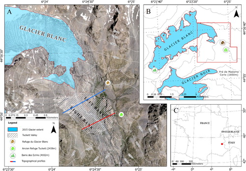
The Tuckett Valley offers an interesting opportunity to study the dynamics of vegetation establishment in various geomorphic and hydrologic context. Indeed, the valley has been progressively freed from ice since 1986 with no re-advances since then, which corresponds to the start of regular satellite observation (Wulder et al., 2019) and to an increase in availability of aerial photography. Furthermore, there is a strong contrast in geomorphic and hydrologic activity potential between the right and left bank of the valley with apparent differences in the spatial distribution of vegetation.

3. Data and methods

3.1. Data sources and corresponding features

To show the connection in space and time between vegetation establishment and glaciological, geomorphological and hydrological features, imagery data from various sources were used.

• Mapping of glacier contours was conducted based on 12 aerial images from the National Institute of Geographic and Forest Information (IGN) historical database (remonterletemps.fr) spanning from 1952 to 2013 and one aerial image of 2015 from © BD ORTHO 2015 Haute-Alpes (05) (geoportail.gouv.fr) available in RGB and IRC type at 50 cm resolution, allowing us to obtain a dense chronosequence of deglaciation. Main characteristics of the historical aerial images are presented in Table 1.

• Hydro-fluvial activity was mapped in 2015 by photo-interpretation using the RGB aerial image of 2015. The 12 aerial images were used to determine the first year of appearance of these previously identified streams.

• A full geomorphology map of the study area was produced based on photo-interpretation of the 2015 aerial photography. The evolution of gullies was followed using the historical aerial imagery highlighting the recent activity.

• Presence/absence of vegetation at high resolution in 2015 was estimated using vegetation index derived from the coloured infra-red aerial image from 2015. Growth rate of vegetation during the 35 last years was assessed using the Landsat time series.

Table 1. Description of the exact date of acquisition, mission ID, spatial resolution and type of the 12 aerials photography extracted from remonterletemps.fr and used to build the chronosequence of deglaciation.

Date	Mission ID	Resolution	Type
01/08/1952	C3435-0081_1952_F3435-3438_0156	1.22 m²	B&W
22/08/1960	C94PHQ3091_1960_F3336-3436_0019	1.06 m²	B&W
21/08/1967	C3435-0111_1967_FR1403_0031	0.4 m²	B&W
29/07/1981	C3435-0024_1981_IFN05_IRC_0400	0.37 m²	IRC
05/09/1986	C3536-0041_1986_F3536-3636_0030	0.56 m²	B&W
27/10/1989	C2205-0551_1989_F3536-3636_0028	0.51 m²	B&W
03/08/1994	CN93000024_1993_IFN05_IRC_1173	0.47 m²	IRC
24/07/1998	CA98S01232_1998_FD38_0029	0.79 m²	RGB
19/07/2000	CA00S01041_2000_F3335-3536_0115	0.58 m²	B&W
11/07/2003	CP03000082_2003_fd0038_250_c_0364	0.89 m²	RGB
05/08/2009	CP09000302_FD05 × 039_02053	0.23 m²	RGB
10/08/2013	CP13000172_13FD0535 × 00010_01790	0.21 m²	RGB
… / … /2015	© BD ORTHO 2015 Haute-Alpes (05)	0.50 m²	RGB/IRC

Note: The aerial photography dated from 2015 and used as reference is also presented.

3.2. Map design

The Main Map intends to represent the connection in space and time between the glacier recession which reveal a new natural arena, the vegetation colonizing it and how intertwined features can control the spatial and temporal distribution of the vegetation. To do so, the mapped features are divided into four themes: Glaciological, geomorphological, hydrological and vegetation. Anthropogenic features are added to the map to improve clarity and link the locator maps and the Main Map. The blue and red topographic profiles are imaginary lines coloured after their historical names (Mougin, 1927).

Glaciological features consist of the chronosequence of deglaciation divided into glacier contours before and after 1986 which corresponds to the last re-advance. Glacier contours after 1986 are multi-coloured as they indicate the approximate year of deglaciation and thus are linked to surface availability for vegetation establishment. Colours were chosen to maximize differentiation between dates. Conversely, glacier contours before 1986 is not linked to surface availability for vegetation establishment and are thus shown in white dashed lines. Glacier extent in 2015 in shown in white to contrast with surrounding bedrock.

The map of geomorphological features is composed of polygons identifying bedrock, stabilized scree area and three different states of moraines (stable, unstable and ice-cored). Gullies are shown using black arrows pointing in the direction of debris flow, and outwash plain using a contoured polygons to accentuate the clear edge of this feature. Contour lines are depicted to show the concave topographic context of the glacier forelands. Colours were chosen to improve overall clarity and differentiation with overlapping features.

Hydrological features are depicted in hues of blue depending on the timing of first observation in the historical aerial image dataset. Presence of vegetation is marked by green pixels while the different hues of green represent various growth rate of vegetation. The 2015 RGB aerial image is used as a base map to add a depth effect.

4. Description of main features

4.1. Chronosequence of deglaciation

Mapping of glacier outlines was conducted by manually geo-referencing, orienting and rectifying the 12 historical aerial images from the IGN (remonterletemps.fr) with the aerial image from 2015 projected in Lambert-93 (EPSG:2154) as the reference. The 13 aerial photographs were from 1952, 1960, 1967, 1981, 1986, 1989, 1994, 1998, 2000, 2003, 2009, 2013 and 2015 with main characteristics presented in Table 1.

The process of geo-referencing was conducted using ArcGIS^® software (Esri, 10.4.1) using spline transformation. The spline method is a true rubber-sheeting method which ensures that all control points in the reference map are geo-referenced to the exact coordinates provided for these locations. This method was preferred as the 12 images were distorted in various ways due to inconsistent view angles and high variations in elevation. Furthermore, it benefits heavily from the amount of control points you have. As the glacier outlines and geomorphology were of most interest, the following methodology was applied:

1. Ten to 50 control points were positioned over locations on the outer boundary and within the image. Roads, consistent topographic features, or refuges were used as references.

2. One hundred fifty to 200 control points were added over the glacier front extent in order to achieve high precision in this particular area.

3. New control points were added to correct for distortion far from the glacier due to step 2.

As the spline transformation method places control points in their exact positions, no direct Root-Mean-Square-Error (RMSE) are computable. Thus, uncertainties associated with geo-referencing could not be quantified directly. Estimating RMS error using more points could be done but would require evenly distributed control points which is not feasible due to lack of identifiable points for image rectification. Thus, superimposition of geo-referenced images was used as visual validation, showing higher accuracy around glacier boundaries, and decreasing accuracy the further you get from the glacier. Through this method, uncertainty can be estimated as ±2 pixels for each image which gives an approximate uncertainty of 2 to 1 m depending on the image (see Table 1). Only the front section of the glacier was mapped, as for many years a single image did not cover the entire glacier (accumulation and ablation areas) and glacier outlines were hardly distinguishable due to persistent snow cover (Figure 2).

Figure 2. New chronosequence of deglaciation from 1952 to 2015. Coloured contours correspond to glacier contours since 1986. Black dashed polygons represent area of uncertainty in glacier contours. Transversal blue and red lines represent the historical topographical red and blue profiles from ‘Administration des Eaux et Forêts’ used in Mougin (1927).

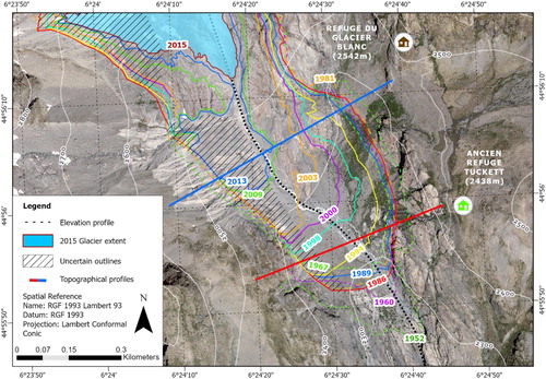
Glacier outlines were manually delineated on ArcGIS^® software (Esri, 10.4.1) for the 13 geo-referenced images by considering the glacier as a mass of ice connected to the accumulation area (Figure 2). Thus, ice disconnected from the main glacier was considered as ‘dead-ice’ which in the context of Glacier Blanc, was only one ice-cored moraine on the right bank of the Tuckett Valley (disconnected from the glacier tongue in approximately 2013). Uncertainties in glacier outlines were assessed as ‘certain’ or ‘uncertain’ based on difficulties during the delineation process. Approximatively 56,500 m² of debris-covered ice located on the right bank of the proglacial area was difficult to map in each year and is the main source of uncertainty. The uncertainties were not presented on the Main Map to improve overall clarity.

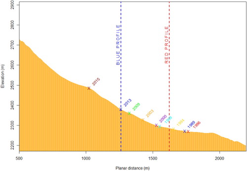
To represent graphically the glacier retreat, an elevation profile was created corresponding to an imaginary central line starting in the accumulation area and ending beneath the Tuckett valley (black dashed line in Main Map). The elevation profile was computed using the Stack Profile tool from the 3D Spatial Analyst extension (ArcGIS) and a Digital Elevation Model (DEM) from RGE ALTI^® Version 2.0 with a 1 m² spatial resolution. Elevation and planar distance from the origin point were measured for each glacier front and for the ‘Administration des Eaux et Forêts’ historical topographical red and blue profiles (Figure 3) used in Mougin (1927).

Figure 3. Elevation profile of a central line crossing glacier fronts from 2015 to 1986. Front positions at all available dates are indicated by crosses, and historical profiles are indicating by dashed vertical lines.

4.2. Geomorphological features

Exhaustive mapping of geomorphological features of the study site was performed using the 2015 aerial image with support from previous work (Lardeux et al., 2015) and field knowledge. It includes bedrock, moraines differentiate by their stability, and scree areas. The stability of moraines was assessed based on local influence of geomorphological features.

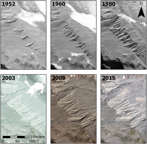
The right bank of the glacier is under the influence of active gullying (Lardeux et al., 2015). The newly georeferenced aerial photography shows that geomorphic activity was still ongoing between 2009 and 2015 (Figure 4). While the glacier was still present in the Tuckett valley, the gullying area supplied the right bank with debris, leading to a difference in rate of melting in the ablation area (Nicholson & Benn, 2006). When the main glacier body retreated from the valley, an ice-cored moraine (Østrem, 1956) remained and kept melting at a lower rate, adding to the instability of the right bank. The contour of the ice-cored moraine in 2015 was identified using streams and contours of the gullying area (Chandler et al., 2018). Under the combined influence of gullies and dead-ice, the moraines present in the debris flow direction is considered as unstable. The main outwash plain impacting vegetation distribution was identified using the 2015 aerial image.

Figure 4. The Glacier Blanc gullying area evolution from 1952 to 2015 highlighting the continuous geomorphic activity supplying the right bank of the proglacial area with debris.

4.3. Hydrological features

Multiple sources of proglacial streams from Glacier Blanc and adjacent glaciers were identified by photo-interpretation of the 2015 aerial image. These proglacial streams united along the principal active channel originating from the tongue of Glacier Blanc. Change in spatial distribution of proglacial streams was assessed between 1952 and 2015 using the historical aerial images. No major change in spatial distribution was observed as all proglacial streams observable in 2015 were present in 1952 considering the gradual glacier recession. As such, time since first observation of each stream was computed showing the contrast between the left bank where streams are present as soon as the deglaciation occurs originating from lateral moraines, and the right bank without observable streams.

4.4. Vegetation establishment and growth

The spatial distribution of vegetation on recently deglaciated areas and surroundings was assessed using a colour infra-red imagery (CIR) from 2015 with a spatial resolution of 50 cm. A Normalized Difference Vegetation Index (NDVI) was computed from the near infra-red and red bands of the CRI using the following formula: $NDVI={\displaystyle \frac{(pNir-pRed)}{(pNir+pRed)}}$where $pNir$ and $pRed$ are the reflectance in the Near Infra-red and red bands, respectively. NDVI ranges from −1 to 1 with pixels considered as vegetated when NDVI was greater than 0. This threshold was calibrated through visual observation.

Vegetation changes during the 35 last years was inferred from Landsat Time Series analysis. This archive provides well-calibrated (Markham & Helder, 2012) and precisely geolocated (Lee et al., 2004) time series of spectral reflectance that span from 1984 to present with a spatial resolution adapted to glacier forelands of 30 m.

Images from Collection 1 were downloaded for all available Landsat scenes from Landsat 5 Thematic Mapper, Landsat 7 Enhanced Thematic Mapper+ and Landsat 8 Operational Land Imager sensors with less than 80% of cloud cover and high geolocation accuracy (geolocation error < 12 m) from 1984 to 2019 through the Landsat Earth Explorer data portal (https://earthexplorer.usgs.gov). Data are downloaded at Surface Reflectance (SR) level of correction, which ensure better time series consistency by eliminating atmospheric effects on reflectance. Clouds and cloud shadows were removed using the Fmask 3.3 currently used by USGS (Zhu & Woodcock, 2012).

This approach allowed an estimation of the chlorophyll activity at a given time and space at a pixel scale. Thus, a significant increase in NDVI over time indicates colonization by vegetation, if vegetation was absent in 1984 (surfaces deglaciated after 1984), or an increase in chlorophyll activity if vegetation was present (surfaces deglaciated before 1984).

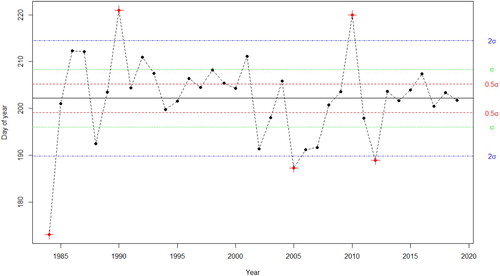
Changes in vegetation were assessed over the 35 years by computing the mean of NDVI available around mid-July (day of year 200 ± 30 days) for each year and pixel, thus producing a map of NDVI mean for each year of the time series over the glacier foreland. Furthermore, the mean of day of year of each pixel was stored and variation through the time series was evaluated. Due to cloud cover and density images (if two satellites are operating at the same time or not) between years, the mean NDVI is not composed of the exact same day for each pixel. Thus, to prevent related errors in NDVI trend estimation, a year is discarded from the greening trend estimation if the mean day of year is superior/inferior to ±2σ of the entire time series (Figure 5).

Figure 5. Mean day of year of retained summer dates over a random pixel for each year of the time series. Black horizontal lines indicate the mean over the entire time series. Coloured dashed lines indicate degree of standard deviation. Red cross corresponds to discarded years according to criteria discussed in the text.

Since time series of NDVI often do not meet parametric assumptions of normality and homoscedacity (Hirsch & Slack, 1984); the Theil-Sen trend estimator was applied for greening trend estimation. The Theil-Sen procedure is a rank-based test that calculates the non-parametric slope and intercept of the series by determining the median of all estimates of the slopes derived from all pairs of observations. This procedure is furthermore resistant to outliers and therefore suitable for assessing the rate of change in short or noisy series (Eastman et al., 2009). The significance of the time series trends was calculated by the non-parametric Mann-Kendall significance test (Eastman et al., 2009). Greening trend estimation is only computed if there is at least 5 valid years per approximatively 11 years (1984–1995, 1996–2008 and 2009–2019) in order to capture the 35 year trends only.

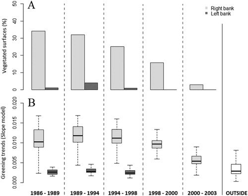
Slope was resampled to the resolution of the CIR for spatial representation on the map and was only displayed for pixels considered as vegetated and with a significant slope (P < 0.05). The percentage of vegetated surfaces by interval of deglaciation was assessed by differentiating the right bank, under the influence of a gullying area, and the left bank, without geomorphic activity, of the valley (Figure 6). Overall, the longer a surface has been deglaciated, the greener it is, which was expected. By comparing the two banks, important differences are observed with very low vegetation coverage for the bank under the influence of geomorphic activity. Also, greening trends were assessed for both banks, and compared to greening trend outside of the glacier foreland. Results shows that the glacier foreland is a hotspot of greening, with strong variability.

Figure 6. (A) The percentage of deglaciated areas colonized by vegetation between 1981 and 2015 for the right (green) and left (red) bank of the Tuckett valley for each interval of deglaciation. (B) The corresponding increases in NDVI per year (median-based linear model slope) estimated from remote sensing for the same interval of deglaciation and for both banks of the Tuckett valley. The greening trend outside of the glacier foreland is shown in dark green for comparison, showing that recently deglaciated areas are hotspots of greening in mountainous landscapes.

5. Discussion

Glacier Blanc offers an interesting opportunity to study spatial variation of vegetation establishment in recently deglaciated terrains with contrasting regimes of disturbance. Since the advance of the glacier ending in 1986, the glacier snout elevation changed from 2270 m to 2540 m a.s.l., leaving more than 100,000 m² of ice-free terrain (Figure 3). Colonization by vegetation was observed over the whole valley but with significant spatial variability. As the left bank was almost completely colonized during the last 35 years with fast increases in productivity, the right bank colonization was more heterogeneous with vegetation patches limited to the lower part of the valley and with slow increases in productivity. The contrast between these two sides of the valley separated by the main river and the outwash plain could be explained in part by the geomorphological context. Compared to the left bank which is not exposed to geomorphic activity above the valley, the right bank is submitted to intense gullying, and to a slow evolving ice-cored moraine underneath. The resulting disturbance regime can explain the slow establishment of vegetation. Also, unlike the right bank, the left bank is exposed to proglacial streams since the first observation available (AD 1952). During the last 70 years, no major changes in spatial distribution of these streams was observed which prevented glacio-fluvial disturbances (Moreau et al., 2005, 2004, 2008) and allowed vegetation succession. Furthermore, nutrient enrichment and high water availability can be expected along channelled and stable streams leading to high vegetation growth.

6. Conclusions

In this paper, we showed the potential of the combination of aerial and satellite remote sensing imageries to study glacier forelands and how vegetation establishment appears to be driven by geomorphological, hydrological and glaciological features. An understanding of the underlying geoecological process could be improved using further field data vegetation (Zimmer et al., 2018) (including species composition, biomass and plant traits) and quantitative estimation of geomorphic or glaciofluvial activities in the glacier forelands and their recent evolution.

This map highlights the pivotal role of local disturbance regime to explain local heterogeneity of vegetation establishment and growth in glacial forelands. Also, it shows the diversity of disturbance context that can be found in a single glacier foreland, and how it interacts to control vegetation establishment pattern and growth on recently deglaciated areas. Medium resolution imageries such as Landsat offers opportunities to study this relation as it offers sufficient spatial resolution adapted to heterogeneous areas difficult to access and a period of activity corresponding to recent deglaciation. This work paves the way for a comparative approach of glacial forelands that will focus on relationships between geomorphic and glaciofluvial activities and greening trends.

Software

Map production and composition were performed using ArcGIS Pro 2.5.1. Geo-referencing has been conducted using ArcGIS^® software (Esri, 10.4.1). Analysis and vegetation indices were computed on RStudio Version 1.1.463.

Acknowledgements

Thanks are due to Emmanuel Thibert and Philippe Choler for their helpful comments on the analysis and this manuscript.

Disclosure statement

No potential conflict of interest was reported by the author(s).

References

- Allix, A. (1922). Les glaciers des Alpes françaises en 1921. Revue de géographie alpine, 10(2), 325–333. https://doi.org/10.3406/rga.1922.1697
- Allix, A. (1929). Observations glaciologiques faites en dauphiné jusqu’en 1924. Les études rhodaniennes, 5, 185–186. https://www.persee.fr/doc/geoca_1164-6268_1929_num_5_1_6727
- Bonnefoy-Demongeot, M., & Thibert, E. (2018, April 01). A century of volume changes of Glacier Blanc (French Alps, Ecrins range) from historical maps and aerial photogrammetry. 22th alpine glaciology meeting, Chamonix, France (hal-02008795), p. 7352.
- Carlson, B. Z., Corona, M. C., Dentant, C., Bonet, R., Thuiller, W., & Choler, P. (2017). Observed long-term greening of alpine vegetation – a case study in the French Alps. Environmental Research Letters, 12(11), 114006. https://doi.org/10.1088/1748-9326/aa84bd
- Chandler, B. M. P., Lovell, H., Boston, C. M., Lukas, S., Barr, I. D., Benediktsson, I. O., Benn, D. I., Clark, C. D., Darvill, C. M., Evans, D. J. A., Ewertowski, M. W., Loibl, D., Margold, M., Otto, J., Roberts, D. H., Stokes, C. R., Storrar, R. D., & Stroeven, A. P. (2018). Glacier geomorphological mapping: A review of approaches and frameworks for best practice. Earth-Science Review, 185, 806–846. https://doi.org/10.1016/j.earscirev.2018.07.015
- Eastman, J. R., Sangermano, F., Ghimire, B., Zhu, H., Chen, H., Neeti, N., Cai, Y., Machado, E. A., & Crema, S. C. (2009). Seasonal trend analysis of image time series. International Journal of Remote Sensing, 30(10), 2721–2726. https://doi.org/10.1080/01431160902755338
- Eichel, J. (2019). Vegetation succession and Biogeomorphic Interactions in glacier forelands in T. Heckmann and D. Morche. Geomorphology of Proglacial Systems, 327–349. https://doi.org/10.1007/978-3-319-94184-4_19
- Eichel, J., Corenblit, D., & Dikau, R. (2016). Conditions for feedbacks between geomorphic and vegetation dynamics on lateral moraine slopes: A biogeomorphic feedback window. Earth Surface Processes and Landforms, 41(3), 406–419. https://doi.org/10.1002/esp.3859
- Eichel, J., Draebing, D., Klingbeil, L., Wieland, M., Eling, C., Schmidtlein, S., Kuhlmann, H., & Dikau, R. (2017). Solifluction meets vegetation: The role of biogeomorphic feedbacks for turf-banked solifluction lobe development. Earth Surface Processes and Landforms, 42(11), 1623–1635. https://doi.org/10.1002/esp.4102
- Eichel, J., Krautblatter, M., Schmidtlein, S., & Dikau, R. (2013). Biogeomorphic interactions in the Turtmann glacier fore field. Switzerland. Geomorphology, 201, 98–110. https://doi.org/10.1016/j.geomorph.2013.06.012
- Filippa, G., Cremonese, E., Galvagno, M., Isabellon, M., Bayle, A., Choler, P., Carlson, B. Z., Gabellani, S., Morra di Cella, U., & Migliavacca, M. (2019). Climatic drivers of greening trends in the alps. Remote Sensing, 11(21), 2527. https://doi.org/10.3390/rs11212527
- Fischer, M., Huss, M., Barboux, C., & Hoelzle, M. (2014). The new Swiss Glacier Inventory SGI2010: Relevance of using high-resolution source data in areas dominated by very small glaciers. Arctic, Antarctic, and Alpine Research, 46(4), 933–945. https://doi.org/10.1657/1938-4246-46.4.933
- Freudiger, D., Mennekes, D., Seibert, J., & Weiler, M. (2018). Historical glacier outlines from digitized topographic maps of the Swiss Alps. Earth System Science Data, 10(2), 805–814. https://doi.org/10.5194/essd-10-805-2018
- Gardent, M. (2014). Inventaire et retrait des glaciers dans les alpes françaises depuis la fin du Petit age glaciaire (PhD dissertation). Université de Grenoble, Grenoble, France. https://www.theses.fr/2014GRENA008
- Hirsch, R. M., & Slack, J. R. (1984). A nonparametric trend test for seasonal data with serial dependence. Water Resources Research, 20(6), 727–732. https://doi.org/10.1029/WR020i006p00727
- Hock, R., Rasul, G., Adler, C., Cáceres, B., Gruber, S., Hirabayashi, Y., Jackson, M., Kääb, A., Kang, S., Kutuzov, S., Milner, Al., Molau, U., Morin, S., Orlove, B., & Steltzer, H. (2019). High mountain areas. In H. O. Pörtner, D. C. Roberts,, V. Masson-Delmotte, P. Zhai, M. Tignor, E. Poloczanska, K. Mintenbeck, A. Alegría, M. Nicolai, A. Okem, B. Petzold, B. Rama, & N. M. Weyer (Eds.), IPCC special report on the ocean and cryosphere in a changing climate, 2, 131–202, In press.
- Lardeux, P., Glasser, N., Holt, T., & Hubbard, B. (2015). Glaciological and geomorphological map of Glacier Noir and Glacier Blanc, French Alps. Journal of Maps, 12(3), 582–596. https://doi.org/10.1080/17445647.2015.1054905
- Lee, D. S., Storey, J. C., Choate, M. J., Hayes, R. W. (2004). Four years of Landsat-7 on-orbit geometric calibration and performance. IEEE Transactions on Geoscience and Remote Sensing, 42(12), 2786–2795. https://doi.org/10.1109/tgrs.2004.836769
- Letréguilly, A., & Reynaud, L. (1989). Past and forecast fluctuations of Glacier Blanc (French Alps). Annals of Glaciology, 13, 159–163. https://doi.org/10.3189/S0260305500007813
- Markham, B. L., & Helder, D. L. (2012). Forty-year calibrated record of earth-reflected radiance from Landsat: A review. Remote Sensing of Environment, 122, 30–40. https://doi.org/10.1016/j.rse.2011.06.026
- Moreau, M., Laffly, D., Joly, D., & Brossard, T. (2005). Analysis of plant colonization on an Arctic moraine since the end of the little ice age using remotely sensed data and a Bayesian approach. Remote Sensing of Environment, 99(3), 244–253. https://doi.org/10.1016/j.rse.2005.03.017
- Moreau, M., Mercier, D., & Laffly, D. (2004). Un siècle de dynamiques paraglaciaires et végétal sur les marges du Midre Lovénbreen, Spitsberg nord-occidental/a century of paraglacial and plant dynamics in the Midre Lovénbreen foreland (northwestern Spistbergen). Géomorphologie: Relif, Processus, Environnement, 10(2), 157–168. https://www.persee.fr/doc/morfo_1266-5304_2004_num_10_2_1211 https://doi.org/10.3406/morfo.2004.1211
- Moreau, M., Mercier, D., Laffly, D., & Roussel, E. (2008). Impacts of recent paraglacial dynamics on plant colonization: A case study on Midre Lovénbreen foreland, Spitsbergen (79°N). Geomorphology, 95(1-2), 48–60. https://doi.org/10.1016/j.geomorph.2006.07.031
- Mougin, P. (1927). Le Glacier Blanc et le Glacier Noir. Études Glaciologiques, 6(1), 157–162. Tome VI. (Cartes 1853, 1880, 1896). https://www.persee.fr/doc/etgla_0983-6500_1927_num_6_1_939
- Nicholson, L., & Benn, D. I. (2006). Calculating ice melt beneath a debris layer using meteorological data. Journal of Glaciology, 52(178), 463–470. https://doi.org/10.3189/172756506781828584
- Nussbaumer, S. U., Nesje, A., & Zumbühl, H. J. (2011). Historical glacier fluctuations of Jostedalsbreen and Folgefonna (southern Norway) reassessed by new pictorial and written evidence. The Holocene, 21(3), 455–471. https://doi.org/10.1177/0959683610385728
- Østrem, G. (1956). Ice melting under a thin layer of moraine, and the existence of ice cores in moraine ridges. Geografiska Annaler, 41(4), 228–230. https://doi.org/10.1080/20014422.1959.11907953
- Paul, F., Barrand, N. E., Baumann, S., Berthier, E., Bolch, T., Casey, K., Frey, H., Joshi, S. P., Konovalov, V., Le Bris, R., Mölg, N., Nosenko, G., Nuth, C., Pope, A., Racoviteanu, A., Rastner, P., Raup, B., Scharrer, K., Steffen, S., & Winsvold, S. (2013). On the accuracy of glacier outlines derived from remote-sensing data. Annals of Glaciology, 54(63), 171–182. https://doi.org/10.3189/2013AoG63A296
- Rabatel, A., Dedieu, J. P., & Reynaud, L. (2002). Reconstitution des fluctuations du bilan de masse du Glacier Blanc (Massif des Ecrins, France) entre 1985 et 2000, par télédétection optique (imagerie Spot et Landsat). La Houille Blanche, 6–7(6-7), 64–71. https://doi.org/10.1051/lhb/2002086
- Raup, B., Racoviteanu, A., Khalsa, S. J. S., Helm, C., Armstrong, R., & Arnaud, Y. (2006). The GLIMS geospatial glacier database: A new tool for studying glacier change. Global and Planetary Change, 56(1–2), 101–110. https://doi.org/10.1016/j.gloplacha.2006.07.018
- Rydgren, K., Halvorsen, R., Töpper, J. P., & Njøs, J. M. (2014). Glacier foreland succession and the fading effect of terrain age. Journal of Vegetation Science, 25(6), 1367–1380. https://doi.org/10.1111/jvs.12184
- Saussure, H.-B. (1779–1796). Travel in the Alps, 4 Volumes.
- Thibert, E., Faure, J., & Vincent, C. (2005). Bilans de masse du Glacier Blanc entre 1952, 1981 et 2002 obtenus par modèles numériques de terrain. La Houille Blanche, 2(2), 72–78. https://doi.org/10.1051/lhb:200502010
- WGMS. (2012). Fluctuations of Glaciers 2005–2010 (Vol. X). Zemp, M., Frey, H., Gärtner-Roer, I., Nussbaumer, S.U., Hoelzle, M., Paul, F. and W. Haeberli (eds.), ICSU (WDS) / IUGG (IACS) / UNEP / UNESCO / WMO, World Glacier Monitoring Service, Zurich, Switzerland: 336 pp. Publication based on database version: https://doi.org/10.5904/wgms-fog-2012-11.
- Wulder, M. A., Loveland, T. R., Roy, D. P., Crawford, C. J., Masek, J. G., Woodcock, C. E., Allen, R. G., Anderson, M. C., Belward, A. S., Cohen, W. B., Dwyer, J., Erb, A., Gao, F., Griffiths, P., Helder, D., Hermosilla, T., Hipple, J., Hostert, P., Hughes, M. J., … Zhu, Z. (2019). Current status of Landsat program, science, and applications. Remote Sensing of Environment, 225, 127–147. https://doi.org/10.1016/j.rse.2019.02.015
- Zhu, Z., & Woodcock, E. C. (2012). Object-based cloud and cloud shadow detection in Landsat imagery. Remote Sensing of Environment, 118, 83–94. https://doi.org/10.1016/j.rse.2011.10.028
- Zimmer, A., Meneses, R. I., Rabatel, A., Soruco, A., Dangles, O., & Anthelme, F. (2018). Time lag between glacial retreat and upward migration alters tropical alpine communities. Perspectives in Plant Ecology, Evolution and Systematics, 30, 89–102. https://doi.org/10.1016/j.ppees.2017.05.003