Engineering geological mapping using airborne LiDAR datasets – an example from the Vinodol Valley, Croatia

ABSTRACT

This paper presents the potential of airborne LiDAR digital terrain model (DTM) for engineering geological mapping in geologically complex and forested area. The multipurpose, comprehensive engineering geological map is created for the pilot area (16.75 km²) located in the Vinodol Valley, Croatia. Eight topographic datasets were derived from 1-m DTM and visually interpreted to identify lithologies and geomorphological processes. In total, 12 engineering geological units, more than 500 landslides, and gully erosion phenomena are outlined in the pilot area. Results confirmed the greatest potential of visual interpretation of LiDAR derivatives for mapping of geomorphological processes in a large scale. On the other hand, this method allowed identification and mapping of engineering formations that are basic engineering geological units appropriate for the medium-scale engineering geological maps. The produced map represents a valuable tool for a wide range of planning and engineering purposes, as well as for geological hazard and risk assessment.

KEYWORDS:

• Engineering geological mapping
• LiDAR DTM
• visual interpretation
• engineering formation
• geomorphological processes
• Vinodol Valley

1. Introduction

LiDAR (Light Detection and Ranging) or ALS (Airborne Laser Scanning) is a modern, optical-mechanical remote sensing technology that uses active laser transmitters and receivers to accurately acquire elevation data (Wehr & Lohr, 1999). The increasing application of LiDAR technology for studies on Earth’s surface topography over the last two decades is due to the capability to produce high-resolution (HR) Digital Terrain Models (DTMs) by automatically filtering of vegetation and all other above the surface objects (Tarolli, 2014). HR LiDAR DTMs have been broadly used within various studies, including the lithological mapping (e.g. Grebby et al., 2010; Notebaert et al., 2009; Paine et al., 2018; Sarala et al., 2015; Webster et al., 2006), identification and mapping of landslides (e.g. Bell et al., 2012; Bernat Gazibara et al., 2019; Chigira et al., 2004; Eeckhaut et al., 2007; Görüm, 2019; Jagodnik et al., 2020a; Petschko et al., 2016; Schulz, 2007), soil erosion processes (Baruch & Filin, 2011; Đomlija et al., 2019a; James et al., 2007), coastal (Biolchi et al., 2016; Sander et al., 2016) and glacial landforms (Smith et al., 2006; Thorndycraft et al., 2016), river valley environments (Jones et al., 2007), and active faults (Chen et al., 2015). However, the literature reveals that there is still a lack of studies that demonstrate the potential of HR LiDAR DTM for preparation of the comprehensive engineering geological maps in a large scale, in geologically and morphologically complex areas covered by dense forest vegetation.

This paper presents the efficient application of 1 × 1 m LiDAR DTM for production of the multipurpose, comprehensive engineering geological map that shows all relevant components of the engineering geological environment (UNESCO/IAEG, 1976), based on visual interpretation of eight different topographic datasets derived from the DTM. The presented Main Map is the first engineering geological map in the Republic of Croatia, produced using the airborne LiDAR data. In total, 12 engineering geological units, more than 500 individual landslides of 10 landslide types (Hungr et al., 2014), and gully erosion phenomena are identified and mapped in the pilot area, and presented on the Main Map. The pilot area (16.75 km²) is located in the Vinodol Valley, in Croatia. It is composed of carbonate and flysch rock mass covered by various superficial deposits, and is densely forested. Engineering description of identified lithologies within engineering geological units is supported by: (i) field reconnaissance mapping carried out on more than 150 sites; (ii) laboratory testing on soil samples taken from the superficial deposits; (iii) analysis of data obtained from archival engineering geological reports (Biondić & Vulić, 1970; Domjan, 1965; Štajduhar, 1976) and geotechnical design for the landslides remediation purposes (Arbanas, 2000, 2002; Grošić, 2013); and (iv) data analysis from 72 exploration boreholes performed between 1964 and 2013. For the central part of the pilot area (approx. 5 km²), the Engineering Geological Map at a scale of 1:5,000 was available (Biondić & Vulić, 1970), which provided preliminary information about landslide types and soil erosion processes predominantly occurring in the study area. Hydrological data on streams, torrents and captured wells are manually digitized from the official state Topographic Base Map (TBM) at a scale 1:5,000, and are also presented on the Main Map.

2. Pilot area

The pilot area (16.75 km²) is located in the central part of the Vinodol Valley (64.57 km²), which is situated in the north-western coastal part of the Republic of Croatia (Figure 1(a)). The Vinodol Valley represents a lower part of the regional morpho-structural unit Klana – Rijeka – Vinodol – Senj (Prelogović et al., 1981), stretching in Dinaric NW-SE direction. The area is predominantly rural, with approximately 50 small settlements situated in the Valley, and it has been inhabited since the prehistoric times (Rogić, 1968). There are more than 30 settlements located in the pilot area, which are connected by two county roads, several local roads and numerous unnamed roads and pathways.

Figure 1. (a) Geographical location; (b) relief map; and (c) simplified geological map of the pilot area (after Šušnjar et al., 1970).

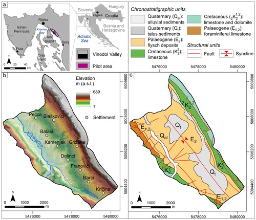
Elevations between 100 and 200 m a.s.l. prevail, and the highest elevations are along the carbonate cliffs that extend along the north-western margin of the pilot area (Figure 1(b)). The prevailing slope angles are between 5° and 20°. The climate is maritime, with the mean annual precipitation between 300 and 700 mm, and maximal precipitation in November. Predominant land covers are dense forests (10.19 km²), shrubs (1.28 km²) and agricultural lands (1.20 km²) (CAEN, 2008).

The Valley flanks are composed of Upper Cretaceous and Palaeogene carbonates, while the lower parts and the bottom of the Valley are built of Palaeogene flysch rock mass (Šušnjar et al., 1970) (Figure 1(c)). These lithologies are predominantly constituted by reverse faults (Blašković, 1999). The Quaternary rockfall breccias (Blašković, 1983) are irregularly distributed along the Valley, and the maximum thickness was observed along the north-eastern Valley margin (Blašković, 1999). Flysch bedrock is almost entirely covered by various types of superficial deposits (Đomlija, 2018; Jagodnik et al., 2020b), formed by geomorphological processes active on slopes in both carbonate and flysch rock mass, such as rock falls, debris flows, debris slides, and gully erosion (Bernat et al., 2014; Đomlija et al., 2017).

The Dubračina River is the main watercourse in the Vinodol Valley, with the total length of approximately 12 km. Its catchment encompasses numerous torrential flows that form within the gullies incised in the flysch bedrock during the intense or prolonged rainfall.

Gully erosion and mass movements are the most significant active geomorphological processes in the Vinodol Valley (Bernat et al., 2014), continuously causing direct damages on public and private properties. Predominantly small and shallow landslides in the Vinodol Valley are mostly developed within the gully landforms (Đomlija, 2018; Jagodnik et al., 2020a).

3. Materials and methods

3.1. Airborne LiDAR datasets

The airborne LiDAR data used in this study were acquired in March 2012, using the multi-return laser scanning system. Point measurements were post-processed and filtered into returns from all objects and vegetation, and returns from the bare ground. The bare ground returns were acquired at the point density of 4.03 points/m² with an average point distance of 0.5 m, and were used for the creation of the 1 × 1 m DTM. The average accuracy of the elevation data is 30 cm.

The LiDAR topographic datasets (i.e. maps) used for identification and mapping of engineering geological units and geomorphological processes were derived from the DTM using standard operations and tools in ArcGIS 10.0 software. These topographic datasets are: (i) the hillshade maps (HM) derived by using different illumination parameters (i.e. 315°/45°, 45°/45°, and 45°/30°), which were additionally overlapped to obtain the optimal shaded relief for each part of the pilot area (e.g. Schulz, 2007); (ii) the slope map (SM); (iii) the contour line maps (CM) derived with the 1-m, 2-m, and 5-m contour line intervals; (iv) the aspect map (AM); (v) the profile curvature map (PrM); (vi) the planform curvature map (PlM); (vii) the stream power index map (SPIM); and (viii) the topographic roughness map (TRM). PrM represents the slope curvature along the lines perpendicular to contours, while PlM reflects the slope curvature on the secant line perpendicular to direction of the greatest inclination (Reuter et al., 2009). The SPIM was calculated according to Moore et al. (1991), using SM and flow accumulation map as input parameters. TRM was calculated according to the slope variability method, which is in detail described in Popit and Verbovšek (2013).

3.2. Visual interpretation of LiDAR topographic derivatives

The visual interpretation of HR LiDAR topographic derivatives was performed in the two steps: (i) preliminary; and (ii) detailed. The preliminary visual interpretation was carried out to determine the possibilities for unambiguous identification and mapping of engineering geological units and geomorphological processes directly from LiDAR maps. It was performed for a portion of the pilot area that was evaluated as representative for its diversity of the lithological and geomorphological features, based on the visual analysis of the HM and field reconnaissance mapping. For this purpose, the LiDAR maps were visually analyzed both individually and in different combinations, e.g. semi-transparent SM over HM; semi-transparent TRM over SM or HM; CM over SM etc., through repeated interpretation phases with the main objective to determine which LiDAR map, or their combination, best reflects a particular lithologic or geomorphic recognition feature. At the same time, field reconnaissance mapping was conducted in order to verify the remote sensing results already in the earliest phase of investigation.

The findings from the preliminary step were used for the detailed visual interpretation, which implies identification and precise manual delineation of engineering geological units and geomorphological processes in the entire pilot area according to established criteria, by one and the same expert. The criteria for identification and mapping are characteristic sets of recognition features indicative for particular lithological and geomorphic phenomena coupled with particular LiDAR maps that are considered to be the most effective for their identification and precise delineation. The main recognition features that have enabled identification of particular lithology and geomorphic phenomena on LiDAR derivatives are: (i) geological structure; (ii) geomorphological setting; (iii) shape; (iv) appearance; (v) morphometric characteristics; and (vi) pattern. For example, elongated or branching shapes, as well as distinct changes in slope angles between the gully channel walls and surrounding slopes visible on SM represent the criteria for identification of gully erosion processes (Đomlija et al., 2019a).

The identification of lithologic and geomorphic phenomena was performed by screening the LiDAR derivatives at scales ranging between 1:1,000 and 1:5,000, relative to the phenomena size. The precise delineation of polygons and lines, however, was carried out in considerably larger scales in order to obtain the high geographical accuracy, ranging between 1:500 and 1:1,000 for engineering geological units and larger gullies, and between 1:100 and 1:500 for landslide and relatively small gully phenomena.

The verification of remote sensing results was performed by multiple field checks during the winter and early spring in 2015 and 2016, in the spars and leaf-off periods. It was conducted for all identified engineering geological units, and for a considerable number of gullies, especially for smaller ones, to avoid their misidentification for forest pathways visible on LiDAR maps. Field checks were partially limited to verification of landslides, because most of them are located in morphologically complex gullies under the forest. Certain landslides located in the gullies could be fully identified from the opposite gully channel walls, from which a desirable distance view could be obtained (Jagodnik et al., 2020a). On the other hand, for a considerable number of landslides at least the landslide crown and main scarp were identified along the gully channel margins, and it was determined the landslide-forming material. For most of the landslides it was difficult to unambiguously identify the landslide type in the field, given that zones of accumulation, the characteristics of which are crucial to determine the type of movement (Soeters & Van Westen, 1996), were difficult to access. However, the specific geomorphological setting of landslides enabled to classify them by applying the principle of uniformitarism (Varnes & IAEG, 1984), given that gullies in this pilot area represent small terrain units characterized by uniform geological and morphological conditions, which resulted in the formation of the same or similar landslide types.

3.3. Soil sampling and laboratory tests

Soil samples from identified superficial deposits were taken at 22 locations, by: (i) manual drilling technique, using an auger and a sampler (ASTM D5680, 2014); and (ii) rectangular soil block sampling technique, using the sampling box (ASTM D7015, 2013). Samples were taken at the subsurface, varying between 0.5 and 1.5 meters depths. Particle-size analysis, liquid-limit test, and plastic-limit test were performed according to the British Standards (BS 13377-2, 2010). The particle-size analysis was performed by the sieve analysis for the coarse-grained, and the hydrometer analysis for the fine-grained soil samples components. All soils were sieved by applying the wet sieving method.

4. Identification and mapping of engineering geological units

There are 12 engineering geological units identified in the pilot area, based on the visual interpretation of LiDAR topographic derivatives (Table 1). Given the attribute of homogeneity of identified lithologies forming the engineering geological units, they represent the engineering formations (Dearman, 1991). Engineering description, symbols and labels of engineering formations are defined according to the general principles of engineering geological mapping given in Dearman (1991). The spatial distribution of the engineering formations identified in the pilot area is presented on Figure 2.

Figure 2. Spatial distribution of the engineering formations identified in the pilot area.

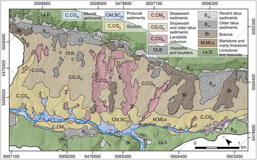
Table 1. Engineering geological mapping units representing the engineering formations (Dearman, 1991) identified in the pilot area, based on the visual interpretation of HR LiDAR topographic derivatives.

Engineering formation		Description			Area (km^2)
Name	Label	Geomorphological setting and origin	Engineering material
Alluvial sediments	C,CGal	Soils in flood plain transported by fluvial processes	Fine grained soil	Clay to gravely clay with subordinate gravel	0.20
Proluvial sediments	CM,SCpr	Soils in proluvial cones transported by gully erosion		Silty clay to clayey sand with subordinate gravel	0.33
Slopewash sediments	C,CMd	Soils in the foot slopes transported by sheet erosion		Clay to silty clay	0.05
Eluvium	C,CGe	Residual soils from weathering of flysch bedrock		Clay to gravely clay with subordinate sand	2.37
Landslide colluvium	C,CGls	Soils in colluvium of large landslides or group of landslides (minimum five successive landslides) with area > 1 ha, gravitationally transported, predominantly by sliding		Clay to gravely clay with subordinate gravel	1.03
Slopewash and older talus sediments	CG,Gd	Soils on flysch bedrock transported by sheet erosion and gravitation	Composite soil	Gravely clay to gravel with many cobbles and boulders	3.79
Olistoliths and boulders	Ol,B	Soils in individual distal sedimentary bodies gravitationally transported, probably by historical rock avalanches	Very coarse composite soil	Olistoliths and massive boulders	0.23
Recent talus sediments	Bs2	Soils in scree cones and scree sheets gravitationally transported, predominantly by active rock falls and rock topples		Small to massive boulders with some fine soils	0.53
Older talus sediments	Bs1	Soils in scree cones and scree sheets gravitationally transported, predominantly by historical rock falls, rock topples and rock avalanches		Small to massive boulders with much finer soils; sediments are semi-lithified in places	1.30
Breccia	Br	Rudaceous sedimentary rock with carbonaceous detritus lithified by carbonate cement; massive	Rock	Weak to moderately strong rock	1.03
Marlstone and marly limestone	M,MLs	Carbonate-rich argillaceous sedimentary rock; thinly to thickly bedded		Weak to moderately strong rock	0.03
Limestone and dolomite	Ls,D	Carbonaceous sedimentary rock; thinly to thickly bedded, and massive		Strong rock	11.54

The elements of geological structure, that can be easily recognized on HM, as well as the rough texture expressed on TRM, are the main recognition features for distinguishing the engineering formation of limestone and dolomites from other lithologies, in particular from the recent talus sediments (Figure 3(a)). The latter formation is identified in the foot of the limestone and dolomite slopes, in the form of cone shaped and steeply inclined sedimentary bodies recognizable on CM and SM, as well as according to the smooth appearance visible on TRM. Engineering formation of older talus sediments can be also easily identified on CM (Figure 3(a)). Their rougher texture and gentler slopes enabled the identification of the boundary between the formations of the older talus and recent talus sediments.

Figure 3. Visualization of topography of the engineering formations identified in the pilot area on HR LiDAR derivatives, presented on: (a) the hillshade map (HM) without interpreted engineering formation boundaries; (b) the topographic roughness map (TRM); and (c) the contour line map (CM) over the slope map (SM), with delineated engineering formation boundaries.

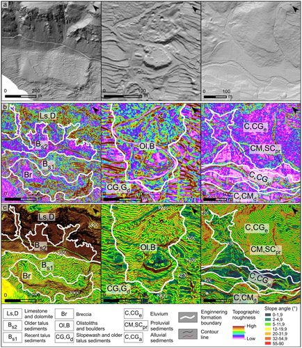
The patchy occurrence of breccia outcrops can be easily recognized already on HM (Figure 3(a)). The rough texture and the abrupt changes in slope angles along breccia margins can be clearly recognized on TRM and SM. These maps, mostly coupled with CM, enabled a precise delineation of engineering formation of breccia in the pilot area. The same maps are also the most effective for identification and mapping of the engineering formation of olistoliths and boulders, given that their appearances, shapes and morphometric characteristics are similar to those of the breccia (Figure 3(b)). Although the combined interpretation of TRM, SM and CM enabled high geographical accuracy of delineated engineering formation boundaries, field reconnaissance was necessary for unambiguous lithological identification of both the breccia and the olistoliths and boulders, due to the significant morphological convergence on LiDAR derivatives.

Geomorphological setting was the most relevant recognition feature for identification of the alluvial sediments in flood plain, the proluvial sediments at the gully mouths, and the slopewash sediments accumulated at the foot of the eluvium formed on flysch bedrock (Figure 3(c)). These engineering formations could have been easily identified and delineated based on the visual interpretation of SM coupled with CM, because these maps clearly reflect the fan shaped and gently inclined sedimentary bodies, in contrast to the flattened terrain in flood plain.

The engineering formation of slopewash and older talus sediments could be unambiguously identified only in the field. This is due to the lack of distinctive shapes and specific morphometric characteristics of sedimentary bodies recognizable on LiDAR maps. However, the specific terracing pattern (Figure 3(b)) was the main recognition feature for identification of the slopewash and older talus deposits, because cultivated land in the pilot area is mostly located within this engineering formation. As the boundaries of this unit cannot be mapped directly from LiDAR derivatives, they are indirectly determined after the mapping of the adjacent engineering formations. The engineering formation of landslide colluvium (Table 1; Figure 2) was delineated after finishing identification and mapping of landslides. However, the landslide colluvium is not presented in the Main Map, as there are presented the individual landslide phenomena that form this engineering formation.

5. Identification and mapping of geomorphological processes

Gully erosion and different types of landslide phenomena are identified in the pilot area, based on the visual interpretation of HR LiDAR derivatives (Đomlija, 2018). The whole methodology for identification and mapping of gully erosion using the visual interpretation of HR LiDAR DTM is presented in Đomlija et al. (2019a), while the methodology for identification and mapping of landslides using the same method is described in Đomlija et al. (2019b) and Jagodnik et al. (2020a).

Gullies are distinguished into two groups according to their width: (i) gullies > 3 m wide, which are mapped by polygons representing the gully channel and lines representing the gully thalweg; and (ii) gullies < 3 m wide, which are mapped by lines representing the gully thalweg. Gully width was manually measured on SM along the imaginary line with ends located at the points of the distinct change of slope angle (Casalí, Giménez & Campo-Bescós, 2015), in the gully channel part that was visually evaluated to be the narrowest. The 3-meter threshold for mapping gullies was chosen because width of gullies narrower than 3 m is only two or three pixels.

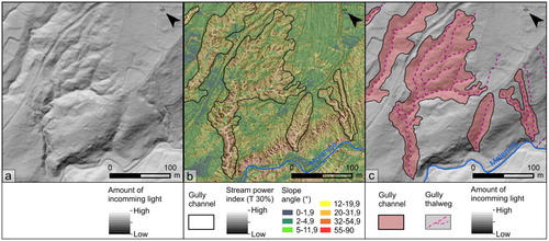
An elongated and branched shape is the main recognition feature for direct and unambiguous identification of gully elements on LiDAR maps, which can be easily recognized already on HM (Figure 4(a)), even for the smallest gully forms. The SM is the most effective LiDAR map for delineation of the gully channels, due to the abrupt changes in slope angles between the gully channel walls and surrounding slopes (Figure 4(b)). The best reflection of the linear shape of the gully thalwegs is on SPIM, which can be recognized and digitized along the lines of the highest stream power index (Figure 4(b)). The visual interpretation of as well the PrM and PlM is also effective for identification and mapping of gully elements (Đomlija et al., 2019a). In total, 31 gully polygons are delineated, with the total area of 1.44 km². The smallest gully channel in the pilot area has an area of 317 m², the largest 0.48 km², while the average has an area of 6,700 m². The area of 75% of identified gullies is smaller than 35,568 m².

Figure 4. Visualization of topography of the gully erosion phenomena identified in the pilot area on HR LiDAR derivatives: (a) the hillshade map (HM); (b) the semi-transparent (40%) slope map (SM) over the stream power index map (SPIM); and (c) the hillshade map (HSM) with delineated polygons representing the gully channels, and lines representing the gully thalwegs.

During the mapping, landslides are classified into 10 types (Table 2), according to the updated Varnes classification of landslide types (Varnes, 1978) proposed by Hungr et al. (2014). The type of movement is determined based on the shape of a delineated polygon, and distinctive topographic characteristics of landslide features specific for particular landslide kinematics (Soeters & Van Westen, 1996) visible on LiDAR derivatives. For example, translational sliding was identified based on predominantly elongated polygons and hummocky runout, whereas the step-like landslide topography and back-tilted head were indicative for rotational sliding. The landslide depth is estimated based on the polygon size (Cruden & Varnes, 1996). The type of landslide material is determined based on the lithology of identified engineering formations.

Table 2. Landslide types according to Hungr et al. (2014) identified in the pilot area. Information on delineated landslide features is given for each landslide types, as well as descriptive statistics on landslide area.

Landslide type (Hungr et al., 2014)		Delineated landslide features	Total number	Atot (km^2)	Amin (m^2)	Aavg (m^2)	Amax (m^2)
Rock fall and rock topple	Detachment, fall, rolling and bouncing of rock fragments, with little dynamic interaction between moving fragments.	Cliff and slope face	–	1.44	–	–	–
	Forward rotation and overturning of rock columns or plates, separated by steeply dipping joints.	Chutes	41	0.17	143	4,211	29,831
Rock irregular slide	Sliding of a rock mass on an irregular rupture surface consisting of a number of randomly oriented joints, separated by segments of intact rock.	Zone of depletion	20	0.09	927	4,507	11,827
Rock rotational slide	Sliding of a mass of weak rock on a rotational rupture surface which is not structurally controlled, under the surcharge of a stronger cap rock.	Landslide body	2	0.02	7,062	10,323	10,323
Rotational slide	Sliding of a mass of soil on a rotational rupture surface, with little internal deformation.	Landslide body	5	0.10	3,780	49,462	49,462
Debris slide	Sliding of a veneer of colluvium or residual soil over a harder substrate on a shallow planar surface parallel to the ground.	Landslide body	321	0.62	65	1,989	43,151
Debris slide-debris flow	Movement initiates as a sliding of a veneer of colluvium or residual soil over a harder substrate on a shallow planar surface parallel to the ground, and it transforms into a flow after moving a relatively short distance.	Landslide body	131	0.30	154	2,503	19,923
Debris flow	Flow of saturated debris which occurs periodically on established path, usually steep drainage channel. The movement is specific to a given path and deposition area, and it may be initiated by a rock fall, rock slide or avalanche.	Flow channel	9	0.43	141	42,818	132,103
Debris avalanche	Very rapid shallow flow of partially or fully saturated debris on steep slope, without confinement in an established channel. The movement initiates as debris slide and is associated with failures of residual and colluvial soils.	Landslide body	1	0.05	–	–	–
Rock slope deformation	Deep-seated slow to extremely slow deformation of slope, with development of cracks or faults, without a well-defined rupture surface.	Portion along the tension crack	1	0.006	–	–	–

There are different possibilities for unambiguous identification and mapping of particular landslide types directly from LiDAR derivatives (Table 2). For most of identified landslides, e.g. debris slides, debris slide-debris flows and rotational slides, the whole landslide boundary representing the entire landslide body can be identified and delineated on LiDAR maps, since the topography of landslide features is, more or less, clearly visible on LiDAR derivatives. In contrast, for some landslide types, e.g. rock irregular slides and debris flows formed in carbonate rock slopes and cliffs, only the certain landslide features can be delineated on LiDAR maps. These are mostly the zones of depletion, as well as the debris flow channels, because for most of the landslides initiated along the carbonate rock slopes and cliffs it was not possible to identify individual zones of accumulation (Đomlija et al., 2019b).

Rock falls and rock topples were necessary to identify firstly in the field and then to map on LiDAR maps indirectly, with polygons depicting (Đomlija et al., 2019b): (i) cliff and slope faces, as the source areas for the rock fall and rock topple phenomena; and (ii) chutes, formed at cliff’s portions where the rock falls and rock topples occur more frequently (Selby, 1993) (Table 2). It is also uncertain the actual extent of the phenomenon that is assumed to represent the rock slope deformation, given that the only recognition feature is the tension crack identified above the carbonate cliff. It is visible part from the top of one of the largest chutes (21,851 m²) identified in the pilot area and extends along the carbonate plateau almost parallel to the extension of the cliff, in a length of 136 m (Đomlija et al., 2019b). Due to the lack of other recognition features visible on LiDAR derivatives, as well as more detailed research of this phenomenon, it was possible to delineate only the portion of the carbonate plateau which is surrounded by the tension crack and the upper cliff boundary. Although the geographical accuracy of the delineated boundary is reduced, it is still depicted the portion of the deformed rock slope that may facilitate the development of a compound rock slide (Hungr et al., 2014).

The most abundant landslide phenomena in the pilot area are debris slides (Table 2), typically activated along the contact between the flysch bedrock and superficial deposits (Arbanas, 2000, 2002; Jagodnik et al., 2020a). The delineated debris slide polygons are predominantly elongated, and often have uniform width along the total length. For a particular number of landslides in this pilot area, the initial translational sliding of debris material transformed into a flow after moving a relatively short distance, thus forming debris slide-debris flows. Their polygons often narrow at the transition from the zone of depletion to the zone of accumulation. Flowage features can be generally clearly recognized in the zones of accumulation, based on the hummocky appearance of their lobate convex forms. The total area of debris slide and debris slide-debris flow phenomena identified in the pilot area is 0.92 km² (Table 2). All identified debris slide-debris flows are located within gullies, as well as the most of identified debris slides. The size of the smallest mapped polygon representing the individual landslide (i.e. debris slide) is 65 m², and the largest polygon (i.e. rotational slide) has an area of 49,462 m². Only one landslide phenomenon in the pilot area is considered to represent an open-slope debris avalanche (Table 2), based on its relatively large size and the shape of delineated polygon. This is the largest landslide identified in the Vinodol Valley, with the total length of 443 m (Đomlija, 2018). It was probably initiated by a rapid failure of the thick eluvium, and had a higher velocity than the velocity of other landslides formed in debris material in the study area. Only the topography of the zone of accumulation has been preserved, which can be clearly identified on LiDAR derivatives and in the field. The landslide is still active, as indicated by the continuous damages of the unnamed road passing along the landslide crown.

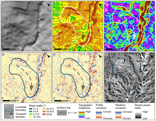
A semilunar landslide crown is easily recognized on SM and CM (Figure 5(b)), for most of the identified landslides. Abrupt changes in slope morphology specific for the main scarp (e.g. steep slope angles and slope concavities) can also be easily recognized on SM, as well as on TRM and PrM (Figure 5(c and d)). A hummocky appearance, rough texture and frequent changes of curvature in a landslide foot are clearly expressed on TRM and PrM (Figure 5(c and d)), for most of the landslides identified in the pilot area (e.g. Jagodnik et al., 2020a). The PlM and SPIM have also enabled a clear recognition of the landslide toes, as well as the landslide tips, in particular when the landslide boundary coincide with the gully thalweg (Figure 5(e and f)).

Figure 5. A representative example of the landslide topography identified in the pilot area on HR LiDAR derivatives: (a) the hillshade map (HM); (b) the contour line map (CM) over the slope map (SM); (c) the topographic roughness map (TRM); (d) the profile curvature map (PrM); (e) the planform curvature map (PlM); and (f) the stream power index map (SPIM).

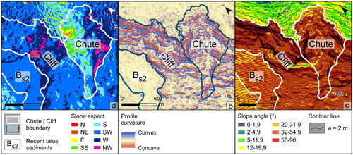
Chutes are identified and mapped based on the visual interpretation of AM (Figure 6(a)), because this map the most clearly reflects the V-shaped channel. Cliff’s topography can be easily identified on PrM and SM (Figure 6(b and c)), relative to the plateau and talus sediments located in the surroundings. The largest part of the upper cliff’s boundary was delineated based on the visual interpretation of SM coupled with CM, while the lower cliff’s boundary was delineated based on the visual interpretation of TRM (Đomlija et al., 2019b), because this map the most clearly reflects the textural differences between the rough cliff’s face and the smoothed talus sediments.

Figure 6. A representative example of the cliff’s face and chute topography indicative for rock falls and rock topples in the pilot area on HR LiDAR derivatives: (a) the aspect map (AM); (b) the profile curvature map (PrM); and (c) the contour line map (CM) over the slope map (SM).

6. Discussion and conclusions

This study demonstrated the efficacy of the airborne 1 × 1 m LiDAR DTM for engineering geological mapping in geologically complex and forested area. The multipurpose, comprehensive engineering geological map (UNESCO/IAEG, 1976) has been produced for the pilot area of 16.75 km², based on the visual interpretation of eight topographic datasets derived from the LiDAR DTM.

Given the applied procedures for identification and mapping of engineering geological units and geomorphological processes carried out in this study, there is a high geographical and thematic accuracy of the remote sensing results. However, the produced engineering geological map cannot be consistently classified according to a scale, given the different possibilities for lithological and geomorphological mapping. Namely, the study confirmed that the visual interpretation of LiDAR derivatives is highly effective for mapping of geomorphological processes in a large scale (e.g. Eeckhaut et al., 2007; Petschko et al., 2016), given the total number of identified and precisely delineated gully and landslide phenomena. Moreover, it was possible to identify 10 different landslide types, according to classification proposed by Hungr et al. (2014). On the other hand, the applied method allowed identification and mapping of engineering geological units only to the rank of engineering formations, which is the appropriate mapping unit rank for the medium-scale engineering geological maps (Dearman, 1991). Although the visual interpretation of LiDAR derivatives efficiently enabled unambiguous identification of most lithologies at the study area, formed under specific geological and geomorphological conditions, more detailed ground investigations and laboratory testing of soil materials are still necessary for interpretation of large-scale engineering geological mapping units or lithological types (Dearman, 1991).

Nevertheless, the results of this study indicate the significant potential of airborne HR LiDAR datasets for detailed engineering geological mapping over the large areas, given the greater possibilities to clearly recognize specific features of particular lithologies and geomorphic phenomena on LiDAR derivatives, in relation to the conventional engineering geological mapping methods. The multipurpose engineering geological map produced for the pilot area in the central part of the Vinodol Valley in Croatia can be applied for various planning and engineering purposes, e.g. land use planning and environmental protection, planning and optimization of site investigations, and preliminary geotechnical design, as well as the base for geological hazard and risk assessment.

Software

The topographic datasets derived from the LiDAR DTM and the comprehensive engineering geological map were originally constructed using ArcMap 10.0. The Main Map was constructed in Corel Draw X6.

Acknowledgement

We kindly thank the reviewers for their constructive comments and suggestions that improved the manuscript and main map.

Disclosure statement

No potential conflict of interest was reported by the authors.

Additional information

Funding

LiDAR data were acquired in the framework of the Croatian-Japanese bilateral project ‘’Risk Identification and Land-Use Planning for Disaster Mitigation of Landslides and Floods in Croatia’’, funded by Japan Science and Technology Agency (JST) and Japan International Cooperation Agency (JICA) through the Science and Technology Research Partnership for Sustainable Development (SATREPS) Program. This work has been supported in part by Croatian Science Foundation under the project ‘’Methodology development for landslide susceptibility assessment for land-use planning based on LiDAR technology’’ (IP-2019-04).

References

- Arbanas, Ž . (2000). Geotechnical design of the County Road CR 5064 Križišće – Tribalj – Grižane – Bribir – Novi Vinodolski, Barci Route (Grižane). Institut građevinarstva Hrvatske, PC Rijeka [in Croatian].
- Arbanas, Ž . (2002). The Ugrini landslide on the County Road CR 5062 Bribir – Lič: Preliminary design. Institut građevinarstva Hrvatske, PC Rijeka [in Croatian].
- ASTM D5680 . (2014). Standard Practice for Sampling Unconsolidated Soils in Drums or Similair Containers.
- ASTM D7015 . (2013). Standard Practices for Obtaining Intact Block (Cubical and Cylindrical) Samples of Soils.
- Baruch, A. , & Filin, S. (2011). Detection of gullies in roughly textured terrain using airborne laser scanning data. ISPRS Journal of Photogrammetry and Remote Sensing , 66 (5), 564–578. https://doi.org/10.1016/j.isprsjprs.2011.03.001
- Bell, R. , Petschko, H. , Röhrs, M. , & Dix, A. (2012). Assessment of landslide age, landslide persistence and human impact using airborne laser scanning digital terrain models. Geografiska Annaler: Series A, Physical Geography , 94 (1), 135–156. https://doi.org/10.1111/j.1468-0459.2012.00454.x
- Bernat, S. , Đomlija, P. , & Mihalić Arbanas, S. (2014). Slope movements and erosion phenomena in the Dubračina river Basin: A geomorphological approach. In S. Mihalić Arbanas , & Ž Arbanas (Eds.), Proceedings of the 1st Regional Symposium on landslides in the Adriatic-Balkan Region: Landslide and flood hazard assessment (pp. 79–84). Croatian Landslide Group – Faculty of Mining, Geology and Petroleum Engineering of the University of Zagreb and Faculty of Civil Engineering of the University of Rijeka.
- Bernat Gazibara, S. , Krkač, M. , & Mihalić Arbanas, S. (2019). Landslide inventory mapping using LiDAR data in the City of Zagreb (Croatia). Journal of Maps , 15 , 773–779. https://doi.org/10.1080/17445647.2019.1671906
- Biolchi, S. , Furlani, S. , Devoto, S. , Gauci, R. , Castaldini, D. , & Soldati, M. (2016). Geomorphological identification, classification and spatial distribution of coastal landforms of Malta (Mediterranean Sea). Journal of Maps , 12 (1), 87–99. https://doi.org/10.1080/17445647.2014.984001
- Biondić, B. , & Vulić, Ž . (1970). The Grižane Landslide 1968 – Engineering geological investigations. Institut za geološka istraživanja, Zagreb [in Croatian].
- Blašković, I. (1983). About distribution and position of pliocene and quaternary sediments at Vinodol. Geološki Vjesnik , 36 , 27–35. [in Croatian].
- Blašković, I. (1999). Tectonics of part of the Vinodol Valley within the model of the continental crust subduction. Geologia Croatica , 52 (2), 153–189. https://doi.org/10.4154/GC.1993.13
- BS 1377-2 . (2010). Methods of test for soils for civil engineering purposes. Classification tests.
- CAEN, Croatian Agency for Environment and Nature . (2008). Corine Land Cover Croatia, Land Use Map 1:100.000.
- Casalí, J. , Giménez, R. , & Campo-Bescós, M. A. (2015). Gully geometry: What are we measuring? Soil , 1 , 509–513. https://doi.org/10.5194/soil-1-509-2015
- Chen, R. F. , Lin, C. W. , Chen, Y. H. , He, T. C. , & Fei, L. Y. (2015). Detecting and Characterizing active Thrust faults and Deep-seated landslides in dense forest areas of Southern Taiwan using airborne LiDAR DEM. Remote Sensing , 7 (11), 15443–15466. https://doi.org/10.3390/rs71115443
- Chigira, M. , Duan, F. , Yagi, H. , & Furuya, T. (2004). Using an airborne laser scanner for the identification of shallow landslides and susceptibility assessment in an area of ignimbrite overlain by permeable pyroclastics. Landslides , 1 (3), 203–209. https://doi.org/10.1007/S10346-004-0029-x
- Cruden, D. M. , & Varnes, D. J. (1996). Landslide types and processes. In A. K. Turner , & R. L. Schuster (Eds.), Landslides, investigation and Mitigation. Transportation research Board, Special Report 247 (pp. 36–75). National Academy Press.
- Dearman, W. R. (1991). Engineering geological mapping . Butterworth-Heinemann.
- Domjan, E. (1965). Technical report on field investigations of the Grižane landslide. Rijekaprojekt, Rijeka [in Croatian].
- Đomlija, P. (2018). Identification and classification of landslides and erosion phenomena using the visual interpretation of the Vinodol Valley digital elevation model . Doctoral dissertation, Zagreb: University of Zagreb, Faculty of Mining, Geology and Petroleum Engineering [in Croatian]. https://dr.nsk.hr/en
- Đomlija, P. , Bernat Gazibara, S. , Arbanas, Ž , & Mihalić Arbanas, S. (2019a). Identification and mapping of soil erosion processes using the visual interpretation of LiDAR imagery. ISPRS International Journal of Geo-Information , 8 (10), 438. https://doi.org/10.3390/ijgi8100438
- Đomlija, P. , Bočić, N. , & Mihalić Arbanas, S. (2017). Identification of geomorphological units and hazardous processes in the Vinodol Valley. In B. Abolmasov , M. Marjanović , & U. Đurić (Eds.), Proceedings of the 2nd Regional Symposium on landslides in the Adriatic-Balkan Region (pp. 109–116). University of Belgrade, Faculty of Mining and Geology.
- Đomlija, P. , Jagodnik, V. , Arbanas, Ž , & Mihalić Arbanas, S. (2019b). Landslide types identified along carbonate cliffs using LiDAR imagery – examples from the Vinodol Valley, Croatia. In M. Uljarević , S. Zekan , S. Salković , & Dž Ibrahimović (Eds.), Proceedings of the 4th Regional Symposium on landslides in the Adriatic-Balkan Region (pp. 91–96). Geotechnical Society of Bosnia and Herzegovina.
- Eeckhaut, V. D. , Poesen, M. , Verstraeten, J. , Vanacker, G. , Nyssen, V. , Moeyersons, J. , van Beek, J. , H, L. P., & Vandekerckhove, L. (2007). Use of LIDAR-derived images for mapping old landslides under forest. Earth Surface Processes and Landforms , 32 (5), 754–769. https://doi.org/10.1002/esp.1417
- Görüm, T. (2019). Landslide recognition and mapping in a mixed forest environment from airborne LiDAR data. Engineering Geology , 258 , 105155. https://doi.org/10.1016/j.enggeo.2019.105155
- Grebby, S. , Cunningham, D. , Naden, J. , & Tansey, K. (2010). Lithological mapping of the Troodos ophiolite, Cyprus, using airborne LiDAR topographic data. Remote Sensing of Environment , 114 (4), 713–724. https://doi.org/10.1016/j.rse.2009.11.006
- Grošić, M. (2013). Landslide on the Local road LR 58075, Podbadanj location. Geotechnical report, Geotech d.o.o., Rijeka [in Croatian].
- Hungr, O. , Leroueil, S. , & Picarelli, L. (2014). The Varnes classification of landslide types, an update. Landslides , 11 (2), 167–194. https://doi.org/10.1007/s10346-013-0436-y
- Jagodnik, P. , Bernat Gazibara, S. , Jagodnik, V. , & Mihalić Arbanas, S. (2020b). Types and distribution of the Quaternary deposits originated from carbonate rock slopes in the Vinodol Valley, Croatia – new insights using airborne LiDAR data. The Mining-Geology-Petroleum Engineering Bulletin , 51 (4), https://doi.org/10.17794/rgn.2020.4.6
- Jagodnik, P. , Jagodnik, V. , Arbanas, Ž , & Mihalić Arbanas, S. (2020a). Landslide types in the Slani Potok gully, Croatia. Geologia Croatica , 73 (1), 13–28. https://doi.org/10.4154/gc.2020.04
- James, L. A. , Watson, D. G. , & Hansen, W. F. (2007). Using LiDAR data to map gullies and headwater streams under forest canopy: South Carolina, USA. Catena , 71 (1), 132–144. https://doi.org/10.1016/j.catena.2006.10.010
- Jones, A. F. , Brewer, P. A. , Johnstone, E. , & Macklin, M. G. (2007). High-resolution interpretative geomorphological mapping of river valley environments using airborne LiDAR data. Earth Surface Processes and Landforms , 32 (10), 1574–1592. https://doi.org/10.1002/esp.1505
- Moore, I. D. , Grayson, R. B. , & Ladson, A. R. (1991). Digital terrain modelling: A review of hydrological, geomorphological, and biological applications. Hydrological Processes , 5 (1), 3–30. https://doi.org/10.1002/hyp.3360050103
- Notebaert, B. , Verstraeten, G. , Govers, G. , & Poesen, J. (2009). Qualitative and quantitative applications of LiDAR imagery in fluvial geomorphology. Earth Surface Processes and Landforms , 34 (2), 217–231. https://doi.org/10.1002/esp.1705
- Paine, J. G. , Collins, E. W. , & Costard, L. (2018). Spatial discrimination of complex, low-relief quaternary Siliciclastic Strata using airborne lidar and Near-surface geophysics: An example from the Texas coastal plain, USA. Engineering , 4 (5), 676–684. https://doi.org/10.1016/j.eng.2018.09.005
- Petschko, H. , Bell, R. , & Glade, T. (2016). Effectiveness of visually analyzing LiDAR DTM derivatives for earth and debris slide inventory mapping for statistical susceptibility modeling. Landslides , 13 (5), 857–872. https://doi.org/10.1007/s10346-015-0622-1
- Popit, T. , & Verbovšek, T. (2013). Analysis of surface roughness in the Sveta Magdalena paleo-landslide in the Rebrnice area. RMZ – Materials and Geoenvironment , 60 , 197–204.
- Prelogović, E. , Blašković, I. , Cvijanović, D. , Skoko, D. , & Aljinović, B. (1981). Seismotectonic characteristics of the Vinodol area. Geološki vjesnik , 33 , 75–93. Zagreb [in Croatian].
- Reuter, H. I. , Hengl, T. , Gessler, P. , & Soille, P. (2009). Preparation of DEM for Geomorphometric analysis. In T. Hengl , & H. I. Reuter (Eds.), Geomorphometry – Concepts, software, applications. Developments in soil science (Vol. 33, pp. 87–120). Elsevier.
- Rogić, V. (1968). Vinodol – contemporary conditions of the regional zonality relations. Croatian Geographical Bulletin , 30 (1), 104–125. [in Croatian].
- Sander, L. , Fruergaard, M. , & Pejrup, M. (2016). Coastal landforms and the Holocene evolution of the Island of Samsø, Denmark. Journal of Maps , 12 (2), 276–286. https://doi.org/10.1080/17445647.2015.1014938
- Sarala, P. , Räisänen, J. , Johansson, P. , & Eskola, K. O. (2015). Aerial LiDAR analysis in geomorphological mapping and geochronological determination of superficial deposits in the Sodankyla region, northern Finland. GFF , 137 (4), 293–303. https://doi.org/10.1080/11035897.2015.1100213
- Schulz, W. H. (2007). Landslide susceptibility revealed by LIDAR imagery and historical records, Seattle, Washington. Engineering Geology , 89 (1-2), 67–87. https://doi.org/10.1016/j.enggeo.2006.09.019
- Selby, M. J. (1993). Hillslope materials and processes . Oxford University Press.
- Smith, M. J. , Rose, J. , & Booth, S. (2006). Geomorphological mapping of glacial landforms from remotely sensed data: An evaluation of the principal data sources and an assessment of their quality. Geomorphology , 76 (1-2), 148–165. https://doi.org/10.1016/j.geomorph.2005.11.001
- Soeters, R. , & Van Westen, C. J. (1996). Slope instability recognition, analysis and zonation. In A. K. Turner , & R. L. Schuster (Eds.), Landslides, investigation and Mitigation. Transportation research Board, Special Report 247 (pp. 129–177).
- Štajduhar, M. (1976). The landslide on the Grižane – Kamenjak road. Geomechanical report, Geotehnika, Institut ‘’Geoexpert’’, Zagreb [in Croatian].
- Šušnjar, M. , Bukovac, J. , Nikler, L. , Crnolatac, I. , Milan, A. , Šikić, D. , Grimani, I. , Vulić, Ž , & Blašković, I. (1970). Basic Geological Map of SFRY 1:100,000, Crikvenica Sheet L33-102. Institut za geološka istraživanja, Zagreb, Savezni geološki zavod, Beograd [in Croatian].
- Tarolli, P. (2014). High-resolution topography for understanding Earth surface processes: Opportunities and challenges. Geomorphology , 216 , 295–312. https://doi.org/10.1016/j.geomorph.2014.03.008
- Thorndycraft, V. R. , Cripps, J. E. , & Eades, G. L. (2016). Digital landscapes of deglaciation: Identifying Late Quaternary glacial lake outburst floods using LiDAR. Earth Surface Processes and Landforms , 41 (3), 291–307. https://doi.org/10.1002/esp.3780
- UNESCO/IAEG . (1976). Engineering geological maps. A Guide to their preparation . UNESCO Press.
- Varnes, D. J. (1978). Slope movements, type and processes. In R. L. Schuster , & R. J. Krizek (Eds.), Landslide analysis and Control, Transportation research Board, Special Report 176 (pp. 11–33). National Academy of Sciences.
- Varnes, D. J. , & IAEG Commision on Landslide and Other Mass Movements . (1984). Landslide hazard zonation: A review of principles and practice . The UNESCO Press.
- Webster, T. L. , Murphy, J. B. , Gosse, J. C. , & Spooner, I. (2006). The application of lidar-derived digital elevation model analysis to geological mapping: An example from the Fundy Basin, Nova Scotia, Canada. Can. J. Remote Sensing , 32 (2), 173–193. https://doi.org/10.5589/m06-017
- Wehr, A. , & Lohr, U. (1999). Airborne laser scanning - an introduction and overview. ISPRS Journal of Photogrammetry and Remote Sensing , 54 (2-3), 68–82. https://doi.org/10.1016/S0924-2716(99)00011-8