Geomorphologic landslide inventory by air photo interpretation of the High Agri Valley (Southern Italy)

ABSTRACT

Landslide inventories provide the knowledge basis for many geomorphological applications and also planning and emergency management. Detailed landslide inventories should also be prepared where pre-existing inventories are available, as knowledge updates. In this paper, we present a new geomorphological landslide inventory for an area of the High Agri Valley, Southern Italian Apennines. The map was prepared through systematic interpretation of historical aerial photographs testing extensive use of anaglyph glasses in StereoPhoto Maker freeware. A total of 2124 landslides were classified based on the type of movement, estimated depth, estimated relative age and three levels of uncertainty, providing landslide attributes and map constraints useful for land planning and hazard studies. The map also documents the relationships between landslides and fluvial landforms of different generations, recording important information to investigate the geomorphological evolution of the area further. We expect that landslide mapping in similar environments will benefit from the workflow here presented.

KEYWORDS:

• Landslide mapping
• landslide inventory
• geomorphology
• quaternary
• Apennines

1. Introduction

Knowledge of the spatial and temporal distribution of landslide phenomena is crucial to investigate landscape evolution and its relationships with human activities and land management. The easiest way for describing the distribution of landslides in a territory is by preparing landslide inventory maps (LIMs). If event landslide inventories portray the distribution of landslides triggered in a territory by a particular event (seismic, meteorological, volcanic or anthropic, Ardizzone et al., 2012, 2007; Giordan et al., 2017), geomorphological inventories can be defined as maps that report the cumulative effect of many events through the last (tens of) thousands of years (Bucci et al., 2016a; Guzzetti et al., 2012).

Due to the importance of landslide mapping to assess landslide susceptibility and hazard, a growing number of LIMs have been compiled (Cignetti et al., 2019; Santangelo et al., 2014) at different scales and by different methods and criteria, mainly scattered over areas where landslides caused victims and damage to infrastructures and cultural heritage (Bentivenga et al., 2015; Giordan et al., 2020; Niculiţă et al., 2016; Zumpano et al., 2020).

Despite the fact that geomorphological LIMs are particularly useful for land management and planning, their widespread use over large areas is rather limited due to their inhomogeneous spatial distribution and the use of different mapping criteria, classifications and methods (Guzzetti et al., 2012).

Here, we present a new geomorphological LIM for the NE mountainous margin of the High Agri Valley, Southern Italy, where landslides of different types and sizes are abundant, and their relationships with the geological structures, although locally documented (Bucci et al., 2019), remain largely under-explored.

2. Study area

The study area extends for 235 km², between 40°16′ and 40°29′N, and 15°44′ and 15°59′E, in Southern Italy (Figure 1(A)). The Bifurno and Pesco streams, flowing from SW to NE into the Camastra river, drains a little part (45 km²) of the area toward NE. Most of the area (190 km²) is drained by the Agri River (Figure 1(B)), which flows from NW to SE and encompasses the NE flank of the upper Agri basin, an NW–SE-trending fault-bounded post-orogenic trough formed in the Quaternary in the central part of the Lucania Apennines (Figure 1(C)).

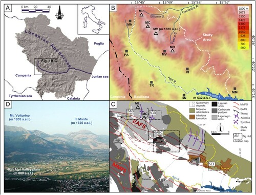
Figure 1. (A) – Geographic location of the study area in the framework of the Lucanian Apennines, Southern Italy. (B) – Elevation map of the study area. Main Mountains (triangles): ML, Mt. Lama; MC, Mt. Calvelluzzo; MV, Mt. Volturino; MO, Il Monte. Main Villages (squares): MN, Marsico Nuovo; PA, Paterno; MV, Marsico Vetere; TR, Tramutola; GN, Grumento Nuova. (C) – Geological and Tectonic sketch map of the study area. The position of the details illustrated in Figures 5 and 6 is indicated. Sketch modified after Giocoli et al. (2015). (D) – Panoramic view of the high Agri Valley plain and the highest mountain in the study area. A four panels figure introduces the study area. Panel A shows a shaded relief of the Lucanian Apennines, in the Basilicata region, Southern Italy. A rectangular box referring to the subsequent panels B and C outlines the middle-west of the region, where the study area is located. Panel B, shows the perimeter of the study area, in the NE side of High Agri Valley, and an elevation map with 11 discrete classes as background. The elevation ranges from 532 m (coastline of Pertusillo lake) to 1835 m (top of Monte Volturino). The study area is elongated in NW–SE direction, as the Agri river, which represents its SE border. The same perimeter of the study area is also reported in panel C, using a schematic geological map as background. The map includes five geo-lithological classes: Quaternary deposits fill the High Agri Valley Plain and characterize the West, South West and South portions of the study area; Miocene siliciclastic dominate its East side, where the Albidona formation crops out in its South East corner. Ligurian Units are only represented in the northern half of the study area, between the Lagonegro units, dominating northward, and the Carbonate platform, which characterize the geology of ‘Il Monte’ and geographically separates the northern and the southern half of the study area. The map also includes five trace symbols indicating relevant sets of geological structures. The NW–SE trending Monti della Maddalena Fault System bounds South East the study area; the NW–SE trending, East Agri Fault System bounds North East the High Agri Valley Plain and longitudinally crosses the study area; Thrusts bound eastward major anticline/syncline pairs involving the Lagonegro units, outcropping in the northern and in the middle-eastern parts of the study area. Four boxes outline important sectors of the study areas: two boxes referring to Figure 5(A–D) are indicated in the north; a large box referring to the Figures 6(A–C) in the centre; a small box referring to the Figure 5(E,F) in the south-east corner. Panel D shows a panoramic photograph of the high Agri Valley plain (m 600 a.s.l.), and the higher two mountains of the study area, Mt. Volturino (m 1835 a.s.l.) and Il Monte (m 1725 a.s.l.), which directly face the plain, giving an idea of the maximum relative relief.

The upper Agri basin is filled by Quaternary continental deposits that cover complex assemblages of pre-Quaternary sedimentary rocks (Giocoli et al., 2015, Figure 1(C)) comprising Mesozoic to Cenozoic platform limestone deposited on top of Upper Triassic dolomite of the Apennine platform domain (Palladino et al., 2008). Clay and sandstone deposited in deep-sea conditions (Liguride and Sicilide units; Bonardi et al., 1988) tectonically overlie carbonate rocks of the Apennine platform domain, which in turn were thrust on top of coeval pelagic rocks of the Lagonegro domain and on younger Miocene synorogenic siliciclastic sediments (Pescatore et al., 1999). Exposure of these rock assemblages dominates the study area, where carbonatic antiformal ridges prevail in the western and central parts, while terrigenous reliefs are widespread eastward.

Elevation in the area ranges from 532 m (coastline of Pertusillo lake) to 1835 m (top of Monte Volturino) with a maximum relative relief approaching 1000 m along the western slopes of the Monte Volturino and Il Monte (Figure 1(B,D)) summits.

3. Methods

The geomorphological LIM was prepared through systematic visual interpretation of two sets of black and white, stereoscopic aerial photographs acquired in 1955 and 2003, both at 1:34,000 scale. The aerial photographs, in digital format at 300 dpi resolution, were interpreted using the freeware StereoPhoto Maker (SPM, http://stereo.jpn.org/eng/stphmkr/) that allows for the anaglyph or shutter glasses 3D view of stereo-pairs. SPM can perform an automatic or manual relative orientation of the images and allows for manual colour adjustments (contrast, light, hue and saturation) and alignment. These features provide the possibility to set up the interpretation work in a few seconds. As a drawback, SPM does not allow yet for any digitisation of features in the 3D environment, but features have to be manually drawn on a topographic base map on the fly. This could introduce some error in the final map in terms of positioning, size and geometry of each landslide, particularly for small ones (Santangelo et al., 2015).

The continuous zoom capability of SPM can be as little as 5% and overcome 200%, which makes it very easy to pass from general overviews to highly detailed views (Figure 2). From this point of view, SPM is more powerful than continuous zoom optical stereoscopes, which usually do not allow general overviews.

Figure 2. Examples of stereoscopic aerial photographs prepared using the freeware StereoPhoto Maker (SPM). (A) – Simultaneous view of more than a single stereo-pair on each display. (B) – Zoom capability of SPM which makes it very easy to pass from general overviews (5%) to highly detailed views (200%). A vertical two panels figure illustrates the digital aerial photographs in anaglyphs mode, prepared using the freeware StereoPhoto Maker (SPM). Panel A shows two computer screens, each displaying two anaglyphs prepared for the photo-interpretation of two different flights. Panel B shows four progressively detailed enlargements, namely of the 5%, 50%, 100% and 200%, of an artificial dammed lake. The images reveal the zoom capability of SPM, which allows for a multiscale investigation of the landscape.

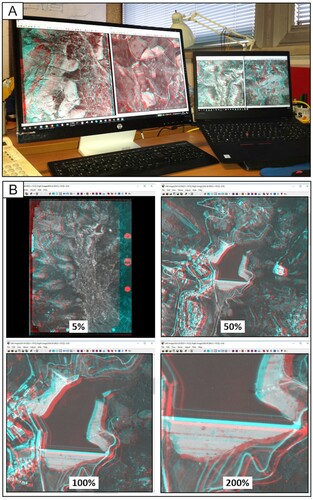
As a further advantage, SPM allows opening multiple instances simultaneously, which allows observing more than a single stereo-pair at once. In this study, we used this feature by loading simultaneously images of 1955 and 2003. Comparing the appearance of the landscape in different epochs can reduce uncertainty in the interpretation. To further reducing subjectivity in mapping, SPM allows for multiple operators examining simultaneously the stereo-pairs, which is comparable to the "discussion" stereoscopes feature. Finally, limited support for polarised glasses makes the use of anaglyph glasses unavoidable, which causes eyestrain in case of intensive use.

Interpretation of the aerial photographs was aided by field surveys and the review of historical and bibliographical data, including geological and geomorphological maps (Bucci et al., 2012; Giano, 2016; ISPRA, in press-a; Zembo, 2010; in press-b), and the available landslide inventories (Lazzari & Gioia, 2016, 2018) produced within a national-scale LIM (Trigila et al., 2010) at 1:10,000 scale.

The geomorphological information was directly drawn on a digital topography, which consisted of a high resolution (1 × 1 m) LiDAR DEM and the 10-m spaced derived contour lines superimposed to it to represent multiscale landforms.

Landslides recognised in the study area were classified according to Cruden and Varnes (1996) and Hungr et al. (2014). In addition, according to WP/WLI (1990, 1993, 1995) landslides were classified based on the estimated depth (as shallow or deep-seated), the inferred relative age (as relict, very old, old or recent), and the degree of uncertainty (identification, delineation and classification). For the deep-seated landslides, the crown area marking the upper part of the depletion zone was mapped separately from the deposit. Finally, the landslide map was completed by mapping other geomorphological elements associated with slope evolution.

3.1. Definition of the legend

An important preliminary step to the preparation of LIMs is the definition of a legend, that is the types of objects that the interpretation will identify and formalise in the map. Information reported in the legend is generally compatible with the (i) techniques used for the landslide inventory making, (ii) morphological characteristic of the area (e.g. the landslide type expected) and (iii) scale of the final map. A legend imposes that interpreters systematically adopt the same scheme for their interpretation, and it prevents non-systematic errors, which are the hardest to correct once the work is at an advanced state.

This paragraph deals with the definition of the legend adopted to classify landslide types of movement (3.1.1), landslide relative age (3.1.2) and the levels of uncertainty in mapping (3.1.3), and other geomorphological features (3.1.4).

3.1.1. Landslide types

Landslide types included in the legend of the LIM are (i) slide, (ii) earth flow, (iii) slide-earth flow, (iv) debris flow, (v) rockfall and (vi) sackung (Figure 3(A)). Within the ‘slide’ item, rotational and translational landslides were considered. Such failures present a well-defined scarp which can be semicircular (rotational slides) or angular (translational slides). The slides deposit is convex in both cases, but it is usually less regular for translational slides. In both cases, it is reasonable to expect a volume balancing between escarpment and deposit areas since slides are usually characterised by low mobility of landslide material.

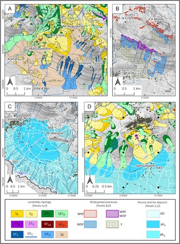
Figure 3. Details of the Main map showing separately the three main groups of geomorphological elements reported in the legend. (A) – Different landslide types; landslide scarp and deposit represented differently. S, slide; SEF slide-earth flow; EF, earth flow; RF, rockfall; DF, debris flow; Sk, sackung. Subscript E, escarpment; subscript D, deposit; subscript C, channel. (B) – Widespread landslide processes; no distinction is made between source and deposit. WRF, widespread rockfalls; WRF/WDF, widespread rock fall/debris flows; WDF, widespread debris flows; T, talus. (C) – Geomorphological elements other than landslides; they include alluvial plain and alluvial fan deposits. AD, alluvial deposits; AF_R, recent alluvial fan; AF_O, old alluvial fan. (D) – Relationships amongst landslides and old and recent alluvial fan deposits. See text for further comments. A four panels figure separately illustrates the main group of geomorphological elements in map, using a shaded relief as background. Panel A, shows a landslide dominated area, where the different landslide types in the legend are all represented. Landslide scarp and deposit are represented differently. Panel B illustrates a detail of Panel A reporting widespread landslide processes, with undistinguished source and deposit, mainly represented by diffuse rockfalls and debris flows along steep slopes, and talus where slope decreases. Panel C shows a recent alluvial fan at the outlet of a high gradient stream, which covers a larger old alluvial fan partially dismantled by minor watercourses draining toward the alluvial deposit and the main course of the Agri River. Panel D shows widespread slides and slide-earth flows, which surround an isolated relief and rest with their feet on the valley floor. Here, several alluvial fans punctuate the outlets of minor streams draining the larger landslide deposits.

Earth flows are landslides characterised by an overall elongated planar shape, with the median part narrower than detachment and accumulation zones. The mobility of earth flows is generally higher than slides, which is also evident in their more elongated shape.

Slide-earth flows are landslides that initiate as slides, then evolving into flows. Therefore, they show the characteristics of slides (most commonly rotational) in the escarpment area, whereas the transport zone and accumulation zone are more similar to earth flows.

Debris flows are rapid-moving landslides that occur along steep slopes. They are shallow features that consist in the detachment of the debris cover along steep slopes due to runoff along channels or open slopes. Levees and tongue-shaped deposits are marked features of the deposition area of debris flows that make them highly recognisable.

Rockfalls are fast-moving landslides that occur along steep rocky slopes. Talus or debris slopes at the foot of sub-vertical cliffs represent the distinctive elements of rock falls.

A sackung is a deep-seated gravitational slope deformation strictly linked to the local tectonic discontinuities (Agliardi et al., 2009; Coltorti et al., 2009 Nemčok, 1972;; Zischinsky, 1969). A slope affected by sackung is gently more convex than surrounding slopes, with the most deformed part generally concentrated at the top, where arched systems of scarps and counter-scarps can be from poorly visible to very well-developed (similar to horst and graben systems).

Other features in the LIM represent areas where individual landslides and slope deposits were too small to be represented at the scale of the map, thus requiring that those features were generalised in, (i) areas affected by debris flow, (ii) widespread rock falls, (iii) associated rockfalls and debris flows and (iv) talus (Figure 3(B)). In the LIM, also linear features are reported, such as debris flow channels and debris flow source areas. They are all features that are unsuitable to draw as a polygon at the publishing scale of the map.

3.1.2. Landslide relative age

Landslides were also classified according to their estimated relative age (sequential panels at the bottom of the Main Map) applying two criteria. The first was indicated by Keaton and DeGraff (1996). According to it, the morphologic and radiometric evidences of landslides become less and less evident (and more difficult to detect) with the increasing age, due to erosion processes and vegetation growth. Such pieces of evidence were also referred to as ‘morphologic and radiometric signature’ by Fiorucci et al. (2018). Depending on this criterion, we identify relict landslides, very old landslides and old landslides. Relict landslides appear dissected, heavily dismantled, so that part of their original border has to be inferred, and they are suspended over the present-day local base level (Migoń et al., 2014). Very old landslides are less dismantled than relict landslides, and they mainly differ from relict landslides because they are yet connected to the present-day local base level. Old landslides appear clearly and poorly to not dismantled or dissected, and their borders appear continuous or solely interrupted by slope failures belonging to subsequent generations. They are connected to the local base level and can show signs of (partial) reactivation in aerial photographs of different epochs. The second criterion adopted to classify landslides relative age is a cross-cut criterion. Younger landslides cover the older ones. This criterion allowed us to detect four landslides generations within the old landslides, one generation within the very old landslides, and two generations within the relict landslides. As opposed to the three major age classes, the minor subdivisions can be applied only to landslides that overlap. Therefore, within the same age class (e.g. ‘old’), no relative age information is given for landslides that have no spatial relationship.

3.1.3. Mapping uncertainty

Uncertainty levels associated with each landslide were also defined, namely, uncertainty in landslide: (i) delineation, (ii) classification and (iii) identification (Panel LU in Main Map). A landslide that was mapped with uncertainty in the delineation was clearly detected and classified. However, at least in some locations along the border, the delineation was not unambiguous, which may have led to mapping errors in the area and/or location and shape of the landslide (Ardizzone et al., 2002). When also classification is involved, it means that even fewer evidences were present to correctly delineating the landslide and defining its type of movement. In this case, there is also a potential thematic error in the final LIM. Finally, in some cases, landslides appear strongly dismantled, their borders are partially inferred as no more evident, and they are particularly large and not unambiguously defined as slope failures (Goetz et al., 2014). In such cases, also uncertainty associated with landslide identification was assigned to the feature reported in the LIM.

Arguably, errors and uncertainties arise and become increasingly important with the increasing age of landslides. This is evident looking at Panel LU in Main Map, where landslides have been coded based on their degree of uncertainty. Only relict and very old landslides show degrees of uncertainty, as opposed to old landslides, which are considered all certain, in delineation, classification and identification.

3.1.4. Other geomorphological features

Finally, other geomorphological features such as alluvial deposits, present-day and relict alluvial fans, and terraces were included in the LIM as geomorphological elements (Figure 3(C)). In particular, alluvial deposits are flat and always located in the lowest portions of the Agri valley and its main tributaries, as they are considered as the present-day alluvial plain deposits. Older deposits of the Agri River valley are nowadays suspended over the alluvial deposits. Furthermore, alluvial fans were recognised and mapped in two relative age classes according to their appearance. They were classified as relict if they look dismantled and dissected, and their border is not completely evident in the aerial photographs due to incision by the present-day river network. Alluvial fans were instead classified as recent if their morphology is well preserved in the present-day morphology. When alluvial fans superimpose each other within the same age class, they were represented within the same relative age class, but according to a cross-cut principle.

Although these features are not directly linked to landslides, they are useful to help geomorphologists identify them. For example, large landslides deposits show the presence of alluvial fans which develop as erosion takes place on landslide deposits (Figure 3(D)).

4. Geomorphological landslide inventory map

Our inventory covers an area of 235 km² and consists of 2124 landslides, for which we obtained the area A_L (in m²) in a GIS in the range 1.16 × 10² < A_L < 1.15 × 10⁷ m². Landslides cover an area of 90.3 km², which represents 38% of the study area. Percentage increases to 52% for the hilly and mountainous portion of the study area (74% of the entire study area), excluding the Agri valley plain. Similarly, the average landslide density throughout the study area is 9 landslides per square kilometre, which rises to 12.2 landslides per square kilometre excluding plain areas.

Descriptive statistics of landslide number and size is shown in Table 1 and Figure 4(A–B). In the first section, Table 1 reveals that slides are the most common landslide types. On average, slides are the larger slope movements, rock falls are the smallest and the less represented. Figure 4(A) shows that relict and very old landslides are not represented by debris flows, rockfalls and earth flows, whose size are typically smaller than those of the other landslide types, e.g. sackungs, slide and slide-earth flow, recognised in the inventory. It appears obvious that small landslides also occurred at the time of very old and relict landslides, but it is reasonable that subsequent landslides and erosion obliterated them. Further evidence emerging from Figure 4(A) is that a large portion of the total landslide area is occupied by a few relict and very old kilometre-scale large slope failures. The evidence was also presented in a paper by Bucci et al. (2016b), showing that the majority of the landslide volume was mobilised in a different morpho-climatic regime.

Figure 4. Plots summarising landslide statistics. (A) – Landslides number (represented by a colour gradient and labels) and cumulated area (proportional to circle sizes), grouped by relative age classes and landslide type (SK, sackung; SEF, slide earth flow; S, slide; RF, rockfall; DF, debris flow; EF, earth flow). (B) – Distribution of landslide areas within each relative age class. The relative age classes are indicated through a letter (R, relict; V, very old; and O, old), and a subscript number that indicates the generation within the age class (1–4). A vertical two panels figure summarises the landslide statistics. Panel A shows a plot having the seven classes of landslide relative age in the abscissa and the six classes of landslide type in the ordinate. In the plot, for each type and relative age class, landslide number is represented by a colour gradient and labels, while cumulated area is proportional to circle sizes. The slide is the most represented landslide type, especially in the first generation of the old class (O1), while rock fall is the less represented. Rock fall, debris flow and earth flow are not represented in the relict and very old classes of relative age. Panel B shows a box plot having the seven classes of landslide relative age in the abscissa, as in panel A, and the landslide area in the ordinate. In the plot, relict and very old landslides show median areas of at least one order of magnitude larger than old landslides (generally two orders of magnitude), while old landslide size range has narrowed asymmetrically through time, with a progressively decreasing size of the larger slope failures, and a median landslide area constant at around 10,000 m².

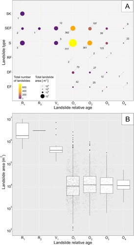
Table 1. Statistic of landslide number and size in the study area.

	Num (#)	Amin (m^2)	Amax (m^2)	Atot (m^2)
Type
Slide	1291	117	11,039,495	81,571,290
Slide-earth flow	642	499	4,157,964	41,197,266
Sackung	1	n/a	n/a	11,559,995
Earth flow	75	907	344,707	1,575,417
Debris flow	110	911	416,012	5,073,676
Rock fall	5	790	27,434	36,187
Landslide relative age
O4	33	2077	60,018	508,095
O3	202	688	352,691	6,253,290
O2	612	531	1,065,125	22,392,748
O1	1253	117	3,013,190	59,291,617
V1	17	143,095	7,991,139	20,345,917
R2	1	Na	na	3,453,469
R1	6	525,377	11,559,995	28,768,698
Landslide uncertainty
Certain	2100	117	3,013,190	88,445,750
Uncertain (delineation)	20	143,095	7,991,139	25,040,843
Uncertain (delineation and classification)	2	1,474,280	3,453,470	4,927,750
Uncertain (delineation, classification and identification)	2	11,039,495	11,559,995	22,599,490

Note: Landslides are classified according to three classification methods, and namely (i) type of movement, (ii) relative age, (iii) uncertainty degree. Landslide number (Num). Landslide area (A). Old landslides: first generation (O1), second generation (O2), third generation (O3) and fourth generation (O4). Very old landslides: first generation (V1). Relict landslides: first generation (R1) and second generation (R2).

As reported in the second section of Table 1 and in Figure 4(A), most of the old landslides (1235) are classified as first-generation, and landslides number progressively decreases with the increase of generation (second to fourth) (Figure 4(A)). Besides, within the clusters of landslides, those of generations higher than the first are typically smaller than those of first generations (Figure 4(B)), suggesting a threshold size effect of previous landslides on subsequent slope movements. In particular, in Figure 4(B), relict and very old landslides show median areas of at least one order of magnitude larger than old landslides (generally two orders of magnitude), while the old landslide size range has narrowed asymmetrically through time, with a progressively decreasing size of the larger slope failures, and a median landslide area constant at around 10,000 m². We interpret these pieces of evidence as the result of local morphological and hydrological perturbations induced by the occurrence of the first failure.

The third section of Table 1 shows the uncertainty degree affecting landslide identification, classification and delineation. Uncertainty in defining the delineation of landslide borders is considered a common feature in mapping very old landslides, whose boundaries are usually deeply dismantled by erosion or covered by more recent slope failures. We acknowledge there is a control of landslide age on the uncertainty degrees in landslide mapping. However, we do not have information on the age of the landslides, and only base our considerations on relative age criteria of classification (Keaton & DeGraff, 1996). Based on landslides morphological appearance (McCalpin, 1984; Wieczorek, 1984) and the findings of recent studies on landslide age in Southern Apennine (Gioia & Schiattarella, 2010) and elsewhere (Pánek et al., 2014), we hypothesise that the majority of the landslides in our study area occurred in the last 10–20 Kyr. However, we cannot exclude that some of the largest landslides, in particular those classified as a relict, are older.

Inspection of the Main Map reveals that the local relief and geological setting control the type and spatial distribution of the landslides. (i) Slides and complex/composite failures are most abundant where clay-rich layers are associated with hard sedimentary rocks. (ii) Earth flows have formed primarily where sheared shales and marls crop out. (iii) Debris flow and rockfall cluster at the toe of the western slopes of Il Monte, Mt. Volturino and Mt. Lama, where relative relief is largest and calcareous rocks prevail. (iv) Large, relict and very old deep-seated landslides are controlled by the spatial arrangement of stratigraphic and tectonic discontinuities, a typical condition for the development of deep-seated landslides in the Apennines (Conforti et al., 2012; Guzzetti et al., 1996). Below, we list and describe several remarkable examples of these landslides which are considered representative of the overall landslide type and size variability recognised in our study area.

1. The pattern of the slide type and complex movements is often associated with their relative position within anticline-syncline pairs. This is clear in the northern part of the study area, where pelagic rocks of the Lagonegro domain are extensively exposed in the Monte Lama – Monte Calvelluzzo anticlinal ridge (ML MC in Figure 1(B–C)). Here, landslides are present along the normal and inverted limbs. Failures on normal limbs occurred either along planar or compound surfaces where the anticlinal limb is less steep or along curvilinear surfaces at the core of minor synclines along very steep limbs. This is the case of the Camporotondo landslide (Figure 5(A,B)), described by Bucci et al. (2013), and included with modification in this inventory. The Monte Lama – Monte Calvelluzzo anticline is bounded on its eastern side by a thrust (Figure 1(C)). Landslides are abundant along the thrust zone, characterised by multiple shear surfaces that separate mostly vertical or overturned bedding at the hanging-wall, from asymmetrical synclines at the footwall (Bucci et al., 2020). In this area, and in a similar structural setting in the study area, synclines mainly involve weak and marl-rich rocks, which concentrate water in the upper part of the slopes and favour the evolution of large slides and slide-earth flows (Figure 5(C–D)).

2. Earth flows are more abundant in the southern portion of the study area, where sheared shales and marls of the Miocene siliciclastics and the Albidona formation crop out (Figure 1). In these flysch complexes, failure initiate usually as translational movements, mainly along bedding interfaces, and can turn into earth flows depending on the local lithological characteristics. Consequently, a large variability of landslide types was mapped at these locations (Figure 5(E)). The relative relief of this sector is lower compared to those in the central and northern part of the area and represents a threshold condition for landslide size, which are also smaller, on average. On the other hand, landslide density is very high here (Main Map). Multiple slides and earth flows are common, which gives the topography its typical hummocky appearance (Figure 5(F)).

3. Debris flows originate where the availability of loose slope breccias is more abundant and particularly: (i) where relative relief is large and calcareous rocks prevail, especially if slopes are affected by pre-existing deep-seated landslides (Figure 5(A–B)); (ii) from talus or scree slopes (Figure 3 (A–B)), (iii) along the shear zone of regional normal faults (Figure 1(C)). The main observations related to debris flows were carried out along the W and SW slopes of Il Monte and Mt. Volturino where all these predisposing factors are clearly recognised (Main Map; see also Figure 6(A)). Commonly, debris flows coexist with rock falls, which occur on largely pre-existing discontinuities in the bedrock such as bedding planes, joints, fault surfaces and related fractures.

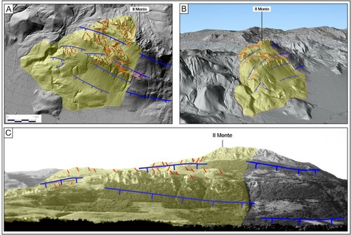
4. In the west side of Il Monte, we mapped diffuse evidences of mountain slope sagging (Figure 6(A)). They include low-lying areas bounded by step, up-slope and down-slope facing escarpments parallel to the mountain crests on the divides and along the slopes. We assigned to the observed sagging phenomenon the maximum level of uncertainty due to the coexistence of morphologic escarpments (Figure 6(B)), supposed to be gravitational in origin, and fault-related scarps (Figure 6(C)) well-recognised and described in the geological literature (Benedetti et al., 1998). Just north of Il Monte, the south and eastern sides of Mt. Volturino are also dominated by other very large and very old failures (Main Map). Similar to the previous case, we assign high levels of uncertainty to these landslides because of the potential morphological convergence resulting from conflicting interpretation (tectonic-driven vs gravitational-driven) of the same landform (Bucci et al., 2014).

Figure 5. Details of the Main map, object of the present study, showing the main landslide types recognised in the study area. The position of the examples is indicated in Figure 1(A) – Multi-generation slide affecting the western slope of the Mt. Lama – Mt. Calvelluzzo Anticline (see text for explanation). (B) – Panoramic view of the area reproduced in A; traces of scarp and deposit of the main slides are indicated; source area of debris flows are outlined in the upper part of the slope. (C) – Multi-generation slide-earth flow affecting the eastern slope of the Mt. Lama – Mt. Calvelluzzo Anticline (see text for explanation). (D) – Panoramic view of the area C; boundary of a wide morphologic depression at the base of the scarp area is indicated. (E) – Variability of landslide types in the SE corner of the study area. (F) – Panoramic view of the largest earth flow represented in E. Legend for maps A, C and E is the same as Figure 3. A six panels figure, organised in three rows and two columns, illustrates the main landslide types recognised in the study area. First column contains three details of the Main map, which are highlighted in the second column by three panoramic photographs. To easily related maps and photographs, the view point of each photograph is indicated in the correspondent map alongside. First row illustrates in map (Panel A) and in panorama (Panel B) multiple slides and debris flow, respectively affecting the lower and upper part of a slope. Second row illustrates in map (Panel C) multiple slide earth flows and subordinated slides, and in panorama (Panel D), a detail of the head of a large slide earth flow deposit. Third row illustrates in map (Panel E) two large old slides partially dismantled and surrounded by numerous slide earth flows and earth flows; the larger earth flow is documented by the picture in Panel F.

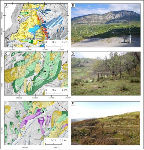
Figure 6. Different views of the large sackung affecting the W–SW slopes of Il Monte. (A) – Plan view of the area, with outlined gravitational-related (red lines) and tectonic-related (blue lines) features. (B) – Perspective view of the same area prepared in the GIS. (C) – Frontal view of the SW slope of Il Monte, where most of the features outlined in A are outlined. A three panels figure illustrates different views of the large sackung affecting the W–SW slopes of Il Monte. In all panels, the sackung is indicated as a yellow partially transparent polygon, the gravitational-related features are outlined with red lines, the normal faults are reported as barbed blue lines indicating the dip direction. Panel A shows a plan view of the area with a shaded relief as background; the view evidences the widespread gravitational-related features recorded in the upper half of the sackung. Panel B shows a perspective view of the same area prepared in the GIS, with the same shaded relief as background; the view outlines the sackung elements with respect to the surrounding landscape. Panel C shows a frontal view of the sackung taken by the Agri Valley Plain; compared to the images in Panels A and B, the photograph emphasises the difficulty to recognise the widespread gravitational-related features, which are the main evidence of the mountain sacking.

5. Conclusions

The new landslide inventory map represents an updated catalogue of landslide phenomena in the High Agri Valley, based on the classification of landslide type and relative age, which provides new data to further investigation of the Quaternary evolution of the landscape of this part of the Southern Apennines. The map was produced thanks to a systematic exploitation of a free non-photogrammetric freeware, StereoPhoto Maker in anaglyph mode for the visual interpretation of two sets of stereo-aerial photographs.

The map also presents a systematic classification of landslides by relative age and uncertainty. A total of seven levels of relative age were identified: two for relict, one for very old and four for old landslides. Analysis of the data revealed that the great majority of landslide volume was mobilised by relict and very old landslides, whereas the landslide maximum size decreased over time and tended to cluster around pre-existing failures. The map also documents previously unreported unknown kilometre-scale relict and very old landslides that mimic the equal-scale geological structure, and the relationships between landslides and other geomorphological elements in the map.

The new inventory map has a large number of potentials uses due to the highly detailed geomorphological information shown.

The landslide information on the map can be used (i) to determine the statistics of landslide size (Malamud et al., 2004), (ii) to trigger detailed studies on types, pattern, and distribution of landslides in relation to geological structures (Guzzetti et al., 1996), tectonic and climatic forcing (Schiattarella et al., 2017), (iii) as a base map for landslide susceptibility and hazard assessment (Guzzetti et al., 2005).

The fluvial related landforms (alluvial deposits, and alluvial fans) can be used as input data to (i) investigate the allometry of old and recent alluvial fans (Mirabella et al., 2018), (ii) study quaternary depositional and erosional events (Mancini et al., 2019), (iii) and in combination with landslide information, study the interplay of gravitational and fluvial processes (Santangelo et al., 2013).

Software

We used (i) Google Earth© (https://www.google.com/earth/) for geo-location of the photo-interpreted data, and for visualisation of the outcrops and of geological and geomorphological sites during the fieldwork, (ii) StereoPhoto Maker (SPM, http://stereo.jpn.org/eng/stphmkr/) for the visual interpretation of the stereo-aerial photographs, (iii) ArcGIS^®10.6 version and QGIS^®3.4 version (http://www.qgis.org/) to digitally organise and analyse the data, and to use the remotely sensed satellite imagery through OGS Web Map Services (WMS), and (iv) to assemble the final map for publication and graphical editing.

Cartographic information

The topographic base map consists of a shaded relief of a LiDAR DEM with GSD of 1 m and contours extracted from the same DEM at a distance of 25 m. All the other features in the topographic maps (elevation points, toponymy, structures and infrastructures) were obtained from the Regional Technical Cartography at 1:10,000 scale. The map is made freely available and usable by the Regione Basilicata GeoPortal (http://rsdi.regione.basilicata.it/viewGis/?project=f8f85db9-54f9-4a61-90f3-49fcaf31a1b2).

Acknowledgements

Authors contribution: Mauro Cardinali (MCA), Francesco Bucci (FB) and Michele Santangelo (MS) performed the photo-interpretation and drafted the geomorphological landslide inventory map. Federica Fiorucci (FF) and Francesca Ardizzone (FA) coded the information in a GIS environment and built a comprehensive geo-database. Daniele Giordan (DG), Paolo Allasia (PA), Davide Notti (DN), Martina Cignetti (MCI), Danilo Godone (DG), and Emilio Norelli (EN) performed the field work. FB, MS, MCA, FF and FA wrote the text and prepared the figures. DN designed the layout of the final map with the support of all the authors. Daniela Lagomarsino (DL) and Alice Pozzoli (AP) checked the final version of the map and the manuscript. Mauro Cardinali (MCA) supervised the research activity.

Disclosure statement

No potential conflict of interest was reported by the author(s).

References

- Agliardi, F., Zanchi, A., & Crosta, G. B. (2009). Tectonic vs. Gravitational morphostructures in the central Eastern Alps (Italy): Constraints on the recent evolution of the mountain range. Tectonophysics, 474(1–2), 250–270. https://doi.org/https://doi.org/10.1016/j.tecto.2009.02.019
- Ardizzone, F., Basile, G., Cardinali, M., Casagli, N., Del Conte, S., Del Ventisette, C., Fiorucci, F., Garfagnoli, F., Gigli, G., Guzzetti, F., Iovine, G., Cesare Mondini, A., Moretti, S., Panebianco, M., Raspini, F., Reichenbach, P., Rossi, M., Tanteri, L., & Terranova, O. (2012). Landslide inventory map for the briga and the giampilieri catchments, NE Sicily, Italy. Journal of Maps, 8(2), 176–180. https://doi.org/https://doi.org/10.1080/17445647.2012.694271
- Ardizzone, F., Cardinali, M., Carrara, A., Guzzetti, F., & Reichenbach, P. (2002). Impact of mapping errors on the reliability of landslide hazard maps. Natural Hazards and Earth System Sciences, 2(1/2), 3–14. https://doi.org/https://doi.org/10.5194/nhess-2-3-2002
- Ardizzone, F., Cardinali, M., Galli, M., Guzzetti, F., & Reichenbach, P. (2007). Identification and mapping of recent rainfall-induced landslides using elevation data collected by airborne lidar. Natural Hazards and Earth System Sciences, 7(6), 637–650. https://doi.org/https://doi.org/10.5194/nhess-7-637-2007
- Benedetti, L., Tapponier, P., King, G. C. P., & Piccardi, L. (1998). Surface rupture of the 1857 southern Italian earthquake? Terra Nova, 10(4), 206–210. https://doi.org/https://doi.org/10.1046/j.1365-3121.1998.00189.x
- Bentivenga, M., Capolongo, D., Palladino, G., & Piccarretta, M. (2015). Geomorphological map of the area between craco and pisticci (Basilicata, Italy). Journal of Maps, 11(2), 267–277. https://doi.org/https://doi.org/10.1080/17445647.2014.935501
- Bonardi, G., Amore, F. O., Ciampo, G., De Capoa, P., Micconet, P., & Perrone, V. (1988). Il complesso Liguride auct.: stato delle conoscenze e problemi aperti sulla sua evoluzione pre-appenninica ed i suoi rapporti con l’Arco calabro. Mem. Soc. Geol. It, 41, 17–35.
- Bucci, F., Cardinali, M., & Guzzetti, F. (2013). Structural geomorphology, active faulting and slope deformations in the epicentre area of the MW 7.0, 1857, Southern Italy earthquake. Physics and Chemistry of the Earth, Parts A/B/C, 63, 12–24. https://doi.org/https://doi.org/10.1016/j.pce.2013.04.005
- Bucci, F., Mirabella, F., Santangelo, M., Cardinali, M., & Guzzetti, F. (2016a). Photo-geology of the montefalco Quaternary Basin, Umbria, Central Italy. Journal of Maps, 12(sup1), 314–322. https://doi.org/https://doi.org/10.1080/17445647.2016.1210042
- Bucci, F., Novellino, R., Guglielmi, P., Prosser, G., & Tavarnelli, E. (2012). Geological map of the northeastern sector of the high Agri Valley, Southern Apennines (Basilicata, Italy). Journal of Maps, 8(3), 282–292. https://doi.org/https://doi.org/10.1080/17445647.2012.722403
- Bucci, F., Novellino, R., Guglielmi, P., & Tavarnelli, E. (2020). Growth and dissection of a fold and thrust belt: The geological record of the High Agri Valley, Italy. Journal of Maps, 16(2), 245–256. https://doi.org/https://doi.org/10.1080/17445647.2020.1737254
- Bucci, F., Novellino, R., Tavarnelli, E., Prosser, G., Guzzetti, G., Cardinali, M., Gueguen, E., & Ivana, A. (2014). Frontal collapse during thrust propagation in mountain belts: A case study in the Lucania Apennines, Southern italy. Journal of the Geological Society, London, 171(4), 571–581. https://doi.org/https://doi.org/10.1144/jgs2013-103
- Bucci, F., Santangelo, M., Cardinali, M., Fiorucci, F., & Guzzetti, F. (2016b). Landslide distribution and size in response to Quaternary fault activity: The peloritani range, NE Sicily, Italy. Earth Surface Processes and Landforms, 41(5), 711–720. https://doi.org/https://doi.org/10.1002/esp.3898
- Bucci, F., Tavarnelli, E., Novellino, R., Palladino, G., Guglielmi, P., Laurita, S., Prosser, G., & Bentivenga, M. (2019). The history of the Southern Apennines of Italy preserved in the geosites along a geological itinerary in the High Agri valley. Geoheritage, 11(4), 1489–1508. https://doi.org/https://doi.org/10.1007/s12371-019-00385-y
- Cignetti, M., Godone, D., & Giordan, D. (2019). Shallow landslide susceptibility, Rupinaro catchment, Liguria (northwestern Italy). Journal of Maps, 15(2), 333–345. https://doi.org/https://doi.org/10.1080/17445647.2019.1593252
- Coltorti, M., Ravani, S., Cornamusini, G., Ielpi, A., & Verrazzani, F. (2009). A sagging along the eastern Chianti Mts., Italy. Geomorphology, 112(1–2), 15–26. https://doi.org/https://doi.org/10.1016/j.geomorph.2009.04.020
- Conforti, M., Robustelli, G., Muto, F., & Critelli, S. (2012). Application and validation of bivariate GIS-based landslide susceptibility assessment for the vitravo river catchment (Calabria, South Italy). Natural Hazards, 61(1), 127–141. https://doi.org/https://doi.org/10.1007/s11069-011-9781-0
- Cruden, D. M., & Varnes, D. J. (1996). Landslides types and processes. Transportation Research Board. Nat. Ac. Sci.
- Fiorucci, F., Giordan, D., Santangelo, M., Dutto, F., Rossi, M., & Guzzetti, F. (2018). Criteria for the optimal selection of remote sensing optical images to map event landslides. Natural Hazards and Earth System Sciences, 18(1), 405–417. https://doi.org/https://doi.org/10.5194/nhess-18-405-2018
- Giano, S. I. (2016). Geomorphology of the Agri intermontane basin (val d’Agri-Lagonegrese National Park, Southern Italy). Journal of Maps, 12(4), 639–648. doi:https://doi.org/10.1002/esp.389810.1080/17445647.2015.1068715
- Giocoli, A., Stabile, T. A., Adurno, I., Perrone, A., Gallipoli, M. R., Gueguen, E., Norelli, E., & Piscitelli, S. (2015). Geological and geophysical characterization of the southeastern side of the High Agri Valley (southern Apennines, Italy). Natural Hazards and Earth System Sciences, 15(2), 315–323. https://doi.org/https://doi.org/10.5194/nhess-15-315-2015
- Gioia, D., & Schiattarella, M. (2010). An alternative method of azimuthal data analysis to improve the study of relationships between tectonics and drainage networks: Examples from Southern Italy. Zeitschrift für Geomorphologie, 54(2), 225–241. https://doi.org/https://doi.org/10.1127/0372-8854/2010/0054-0011
- Giordan, D., Cignetti, M., Baldo, M., & Godone, D. (2017). Relationship between man-made environment and slope stability: The case of 2014 rainfall events in the terraced landscape of the Liguria region (Northwestern Italy). Geomatics, Natural Hazards and Risk, 8(2), 1833–1852. https://doi.org/https://doi.org/10.1080/19475705.2017.1391129
- Giordan, D., Cignetti, M., Godone, D., Peruccacci, S., Raso, E., Pepe, G., Calcaterra, D., Cevasco, A., Firpo, M., Scarpellini, P., & Gnone, M. (2020). A New procedure for an effective management of Geo-hydrological risks across the “Sentiero Verde-Azzurro” Trail, Cinque Terre National Park, Liguria (North-Western Italy). Sustainability, 12(2), 561. https://doi.org/https://doi.org/10.3390/su12020561
- Goetz, J. N., Bell, R., & Brenning, A. (2014). Could surface roughness be a poor proxy for landslide age? Results from the Swabian Alb, Germany. Earth Surf Proc Landf, 39(12), 1697–1704. https://doi.org/https://doi.org/10.1002/esp.3630
- Guzzetti, F., Cardinali, M., & Reichenbach, P. (1996). The influence of structural setting and lithology on landslide type and pattern. Environmental & Engineering Geoscience, II(4), 531–555. https://doi.org/https://doi.org/10.2113/gseegeosci.ii.4.531
- Guzzetti, F., Mondini, A. C., Cardinali, M., Fiorucci, F., Santangelo, M., & Chang, K. T. (2012). Landslide inventory maps: New tools for an old problem. Earth-Science Reviews, 112(1–2), 42–66. https://doi.org/https://doi.org/10.1016/j.earscirev.2012.02.001
- Guzzetti, F., Reichenbach, P., Cardinali, M., Galli, M., & Ardizzone, F. (2005). Probabilistic landslide hazard assessment at the basin scale. Geomorphology, 72(1-4), 272–299. https://doi.org/https://doi.org/10.1016/j.geomorph.2005.06.002
- Hungr, O., Leroueil, S., & Picarelli, L. (2014). The Varnes classification of landslide types, an update. Landslides, 11(2), 167–194. https://doi.org/https://doi.org/10.1007/s10346-013-0436-y
- ISPRA. (In press-a). Carta geologica del Foglio n. 489, Marsico Nuovo, a scala 1:50.000. http://www.isprambiente.gov.it/Media/carg/489_MARSICO_NUOVO/Foglio.html
- ISPRA. (In press-b). Carta geologica del Foglio n. 505, Moliterno, a scala 1:50.000. http://www.isprambiente.gov.it/Media/carg/505_MOLITERNO/Foglio.html
- Keaton, J. R., & DeGraff, J. V. (1996). Surface observation and geologic mapping, in: Landslides: Investigation and mitigation, Transportation Research Board Special Report.
- Lazzari, M., & Gioia, D. (2016). Regional-scale landslide inventory, central-western sector of the Basilicata region (Southern Apennines, Italy). Journal of Maps, 12(5), 852–859. https://doi.org/https://doi.org/10.1080/17445647.2015.1091749
- Lazzari, M., Gioia, D., & Anzidei, B. (2018). Landslide inventory of the Basilicata region (Southern Italy). Journal of Maps, 14(2), 348–356. https://doi.org/https://doi.org/10.1080/17445647.2018.1475309
- Malamud, B. D., Turcotte, D. L., Guzzetti, F., & Reichenbach, P. (2004). Landslide inventories and their statistical properties. Earth Surface Processes and Landforms, 29(6), 687–711. https://doi.org/https://doi.org/10.1002/esp.1064
- Mancini, M., Vignaroli, G., Bucci, F., Cardinali, M., Cavinato, G. P., Giallini, S., Moscatelli, M., Polpetta, F., Putignano, M. L., Santangelo, M., & Sirianni, P. (2019). New stratigraphic constraints for the Quaternary source-to-sink history of the amatrice basin (central Apennines, Italy). Geol. J, 1–26. https://doi.org/https://doi.org/10.1002/gj.3672
- McCalpin, J. (1984). Preliminary age classification of landslides for inventory mapping. Proc. 21st annual Engineering geology & soils Engineering symposium, Moscow, 99–120.
- Migoń, P., Kacprzak, A., Malik, I., Kasprzak, M., Owczarek, P., Wistuba, M., & Pánek, T. (2014). Geomorphological, pedological and dendrochronological signatures of a relict landslide terrain, Mt Garbatka (Kamienne Mts), SW Poland. Geomorphology, 219, 213–231. https://doi.org/https://doi.org/10.1016/j.geomorph.2014.05.005
- Mirabella, F., Bucci, F., Santangelo, M., Cardinali, M., Caielli, G., De Franco, R., Guzzetti, F., & Barchi, M. R. (2018). Alluvial fan shifts and stream captures driven by extensional tectonics in central Italy. Journal of the Geological Society, 175(5), 788–805. https://doi.org/https://doi.org/10.1144/jgs2017-138
- Nemčok, A. (1972). Gravitational slope deformation in high mountains. Proceedings 24th International geological congress, Montreal, Sect. 13, 132–141.
- Niculiţă, M., Mărgărint, M. C., & Santangelo, M. (2016). Archaeological evidence for holocene landslide activity in the eastern Carpathian lowland. Quaternary International, 415, 175–189. https://doi.org/https://doi.org/10.1016/j.quaint.2015.12.048
- Palladino, G., Parente, M., Prosser, G., & Di Staso, A. (2008). Tectonic control on the deposition of the lower Miocene sediments of the Monti della Maddalena ridge (Southern Apennines): Synsedimentary extensional deformation in a foreland setting. Bollettino Della Società Geologica Italiana, 127, 317–335.
- Pánek, T., Hartvich, F., Jankovská, V., Klimeš, J., Tábořík, P., Bubík, M., Smolková, V., & Hradecký, J. (2014). Large late pleistocene landslides from the marginal slope of the Flysch Carpathians. Landslides, 11(6), 981–992. https://doi.org/https://doi.org/10.1007/s10346-013-0463-8
- Pescatore, T., Renda, P., Schiattarella, M., & Tramutoli, M. (1999). Stratigraphic and structural relationships between Meso-Cenozoic Lagonegro basin and coeval carbonate platforms in southern Apennines, Italy. Tectonophysics, 315(1–4), 269–286. https://doi.org/https://doi.org/10.1016/S0040-1951(99)00278-4
- Santangelo, M., Gioia, D., Cardinali, M., Guzzetti, F., & Schiattarella, M. (2013). Interplay between mass movement and fluvial network organization: An example from southern Apennines, Italy. Geomorphology, 188, 54–67. https://doi.org/https://doi.org/10.1016/j.geomorph.2012.12.008
- Santangelo, M., Gioia, D., Cardinali, M., Guzzetti, F., & Schiattarella, M. (2014). Landslide inventory map of the upper Sinni river valley, Southern Italy. Journal of Maps, 1–13. https://doi.org/https://doi.org/10.1080/17445647.2014.949313.
- Santangelo, M., Marchesini, I., Bucci, F., Cardinali, M., Fiorucci, F., & Guzzetti, F. (2015). An approach to reduce mapping errors in the production of landslide inventory maps. Natural Hazards and Earth System Sciences, 15(9), 2111–2126. https://doi.org/https://doi.org/10.5194/nhess-15-2111-2015
- Schiattarella, M., Giano, S. I., & Gioia, D. (2017). Long-term geomorphological evolution of the axial zone of the Campania-Lucania Apennine, Southern Italy: A review. Geologica Carpathica, 68(1), 57–67. https://doi.org/https://doi.org/10.1515/geoca-2017-0005
- Trigila, A., Iadanza, C., & Spizzichino, D. (2010). Quality assessment of the Italian landslide inventory using GIS processing. Landslides, 7(4), 455–470. https://doi.org/https://doi.org/10.1007/s10346-010-0213-0
- Wieczorek, G. F. (1984). Preparing a detailed landslide-inventory map for hazard evaluation and reduction. Bulletin of the Association of Engineering Geologists, 21(3), 337–342. https://doi.org/https://doi.org/10.2113/gseegeosci.xxi.3.337
- WP/WLI – International Geotechnical societies’ UNESCO Working Party on World Landslide Inventory. (1990). A suggested method for reporting a landslide. Bulletin of the International Association of Engineering Geology, 41(1), 5–12. https://doi.org/https://doi.org/10.1007/BF02590201
- WP/WLI - International Geotechnical societies’ UNESCO Working Party on World Landslide Inventory. (1993). A suggested method for describing the activity of a landslide. Bulletin of the International Association of Engineering Geology, 47(1), 53–57. https://doi.org/https://doi.org/10.1007/BF02639593
- WP/WLI - International Geotechnical societies’ UNESCO Working Party on World Landslide Inventory. (1995). A suggested method for describing the rate of movement of a landslide. Bulletin of the International Association of Engineering Geology, 52(1), 75–78. https://doi.org/https://doi.org/10.1007/BF02602683
- Zembo, I. (2010). Stratigraphic architecture and quaternary evolution of the Val d’Agri intermontane basin (Southern Apennines, Italy). Sedimentary Geology, 206–234. https://doi.org/https://doi.org/10.1016/j.sedgeo.2009.11.011, 2010
- Zischinsky, Ü. (1969). Über sackungen. Rock Mechanics, 1(1), 30–52. https://doi.org/https://doi.org/10.1007/BF01247356
- Zumpano, V., Ardizzone, F., Bucci, F., Cardinali, M., Fiorucci, F., Parise, M., Pisano, L., Reichenbach, P., Santaloia, F., Santangelo, M., Wasowski, J., & Lollino, P. (2020). The relation of spatio-temporal distribution of landslides to urban development (a case study from the Apulia region, Southern Italy). Journal of Maps, 1–8. https://doi.org/https://doi.org/10.1080/17445647.2020.1746417