Glacial and periglacial geomorphology of central Troms and Finnmark county, Arctic Norway

ABSTRACT

Here we present a glacial and periglacial geomorphological map of a ∼6800 km² region of central Troms and Finnmark county, Arctic Norway. The map is presented at a 1:115,000 scale with the aim of characterising the spatial distribution of glacial and periglacial landforms and facilitating the reconstruction of the glacial history of the region during the latter stages of deglaciation from the Last Glacial Maximum and into the Holocene. Mapping was conducted predominantly by manual digitisation of landforms using a combination of Sentinel-2A/2B satellite imagery (10 m pixel resolution), vertical aerial photographs (<1 m pixel resolution), and Digital Elevation Models (10 and 2 m pixel resolution). Over 20,000 individual features have been mapped and include moraines (subdivided into major and minor moraines), ridges within areas of discrete debris accumulations (DDAs), flutings, eskers, irregular mounded terrain, lineations, glacially streamlined bedrock, possible glacially streamlined terrain, pronival ramparts, rock glaciers (subdivided into valley wall and valley floor, and rock glacierised moraines), lithalsas, contemporary glaciers and lakes. The map records several noteworthy large moraine assemblages within individual valleys, forming inset sequences from pre-Younger Dryas limits up to the 2018/19 ice margins and represents a valuable dataset for reconstructing Holocene glacial and periglacial activity.

KEYWORDS:

• Glacial geomorphology
• periglacial geomorphology
• remote sensing
• Arctic
• Norway
• Scandinavian Ice Sheet

1. Introduction

Since the retreat of the Scandinavian Ice Sheet (Hughes et al., 2016; Mangerud, 2004) over continental Norway, the Norwegian Arctic has been subject to a complex pattern of glacial advance and retreat cycles (see Nesje, 2009; Solomina et al., 2015 and references therein). The multitude of large scale, and sometimes rapid, glacier fluctuations has produced a complex landscape signature of glacial and periglacial features and surficial materials (Olsen et al., 2013). However, the most recent glacier advance during the Little Ice Age (typically within the past ∼200 years: Ballantyne, 1990; Leigh et al., 2020) is thought to have been the most extensive neoglacial advance and has likely overridden glacial deposits formed during the mid- to late-Holocene (cf. Matthews et al., 2000, 2005).

Norway has a rich history of glaciological and geological investigations with fjords of northern Norway having been studied since the late-1800s/early-1900s (e.g. Grønlie, 1931; Helland, 1899; Vogt, 1913). Detailed investigations into the bedrock geology and Quaternary surficial geology have also been carried out across the region, chiefly funded and compiled by the Geological Survey of Norway (Norges Geologiske Undersøkelse: NGU). There have also been several glacier inventories providing information regarding their characteristics and local geomorphology (e.g. Østrem et al., 1973; Andreassen et al., 2012b). However, while there is good knowledge about the Quaternary history, the patterns and extent of mountain glaciation across Arctic Norway throughout the Holocene, remains less well examined, especially when compared to southern Norway, or the European Alps. Indeed, within central Troms and Finnmark county only a small number of detailed, site-specific studies have been undertaken with the aim of reconstructing glacier change since the termination of the Younger Dryas. Areas covered include Ullsfjord (e.g. Holmes & Andersen, 1964), Lyngenfjord (e.g. Andersen, 1968), the Lyngen peninsula (e.g. Bakke et al., 2005; Ballantyne, 1990), the Bergsfjord Peninsula (e.g. Evans et al., 2002; Wittmeier et al., 2015), the Rotsund Valley (Leigh et al., 2020), and the island of Arnøya (Wittmeier et al., 2020). Most of the more isolated mountain and plateau regions of central Troms and Finnmark county have received little or no attention.

To decipher the intricate assemblages of individual landforms and improve our understanding of the complex mountain and fjord landscape of central Troms and Finnmark county, we have produced a comprehensive, high-resolution (e.g. <1 m) map of the regions glacial and periglacial geomorphology (Main Map). The resulting dataset of this Arctic landscape will provide the foundation for new interpretations of mountain glacier dynamics and landscape response to deglaciation since the termination of the Younger Dryas (∼11,700 yrs. BP; Lohne et al., 2012), throughout the Holocene and up to the present day, further refining existing models of mountain glacial landsystems and their use in paleoglaciological reconstructions (e.g. Benn et al., 2003; Bickerdike et al., 2018; Chandler & Lukas, 2017; Chandler et al., 2019; Darvill et al., 2017; Evans et al., 2002, 2016a, 2016b, 2017a, 2018; Hättestrand & Clark, 2006; Martin et al., 2019). Moreover, the mapping of periglacial landforms provides a baseline for a refined understanding of their development, particularly for some of the more controversial, hybrid landforms, such as rock glaciers, that evolve from a range of antecedent conditions and hence demonstrate equifinality (Berthling, 2011; Evans, 1993; Whalley & Martin, 1992). Additionally, the mapping and monitoring of the development of periglacial landforms remains important, especially in Arctic and alpine environments, as it is likely that periglacial processes will play an increasingly dominate role in landscape evolution in the future (e.g. Ravanel & Deline, 2011; Huggel et al., 2012; Stoffel & Huggel, 2012; Ballantyne, 2018). The increasing prevalence of periglacial processes will likely result in new and/or increased risk to communities within the periglacial domain (e.g. Arenson & Jakob, 2015; Eriksen et al., 2018; Hjort et al., 2018; Jaskólski et al., 2017; Matthews et al., 2018 Stoffel et al., 2014).

In addition to its employment in landsystem developments and applications, this map will also underpin reconstructions of glacial chronologies for the central Troms and Finnmark region, an Arctic area with a cryospheric system particularly susceptible to rapid climate change (IPCC, 2019). This extends the findings of Evans et al. (2002) and Rea and Evans (2007), whose work across the Bergsfjord Peninsula (∼12 km north-east of this study area) illustrated the value of comprehensive landsystem mapping across a whole glacierised region with a topographic complexity that dictates the variable nature of post Younger Dryas glacier-climate responses and hypsometric change in mountain glacier systems, particularly in plateau icefield and fjord head settings.

2. Study area and previous work

The mapping conducted in this study focuses on an area of central Troms and Finnmark county (in the northern region of the former Troms county), between ∼69°11′–70°02′N and ∼19°28′–21°50′E (Figure 1). Geographically, the area extends from the Lyngen Peninsula (otherwise known as the Lyngen Alps) in the west, to the large valley, Navitdalen in the east; and includes the small, glaciated islands of Uløya and Kågen in the north (Figure 1). The region is predominantly characterised by alpine and plateau-type mountain terrains (reaching an altitude of 1834 m a.s.l; at Jiehkkevárri 69°28′N–19°52′E) with steep-sided valleys and fjords in coastal areas, contrasting with inland terrain to the south/south-east comprising an elevated plateau stretching across to the Norwegian border. There is also a considerable west–east precipitation gradient across the study area for example, between 1966 and 2019 total yearly precipitation averages ∼997 mm yr^-1 to the west of our study area (station No. 90490) whereas at the eastern margins (station No. 92350) the total yearly precipitation averages less than half that of the west at only ∼468 mm yr⁻¹.

Figure 1. Location map showing the study site (within the red frame) in central Troms and Finnmark county, northern Norway, with site location within Norway shown on the insert map. The inset outlines show the most credible margin of the Scandinavian Ice Sheet as it retreats inland at 1000-year intervals as reconstructed by Hughes et al. (2016). The base image is a composite of 2 m resolution hill-shaded Arctic DEM tiles and the glaciers are shown using glacier outlines from the Inventory of Norwegian Glaciers (Andreassen et al., 2012).

Map showing the location of the study area in northern Norway with glaciers marked and inset outlines demarcating the former extent of the Scandinavian Ice Sheet.

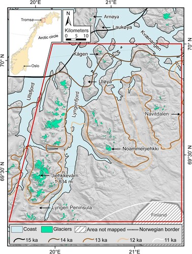
The three largest fjords in the study area are Ullsfjorden (75 km long) and Lyngenfjord (82 km long) flanking the Lyngen Peninsula (to the west and east respectively), and Kvænangen (72 km long). Glaciers are found in the small mountain ranges that boarder the fjords particularly on the Lyngen Peninsula (Andreassen et al., 2012; Stokes et al., 2018), and most are valley and cirque glaciers (some connected with several units as glacier complexes such as Strupbreen and Koppangsbreen, IDs 200 and 205 respectively), with several plateau icefields (Rea et al., 1999; Stokes et al., 2018; Whalley et al., 1981), and one small ice cap (Noammerjiehkki, ID 158). In this paper, we use the glaciers IDs and names following the Inventory of Norwegian glaciers (Andreassen et al., 2012). Beyond the glacierised areas, most of the land surface is underlain by permafrost, with the lower altitudinal limit of sporadic permafrost potentially reaching as low as ∼150 m a.s.l. (Gisnås et al., 2017). Much of the mountain and highland plateau within the study area is, therefore, within the periglacial domain, evidenced by large areas of gelifluction sheets and/or patterned ground and the periglacial reworking of glacial landforms (e.g. permafrost creep or rock glacierisation of moraines; cf. Ó Cofaigh et al., 2003; Evans, 1993; Evans et al., 2016a; Vere & Matthews, 1985).

During the last glaciation, the uplands and fjords throughout the area were covered by the Scandinavian Ice Sheet, with the most credible position of the ice sheet margin terminating near the continental shelf ∼16,000 yrs BP (Hughes et al., 2016). The northern margin of the study area was deglaciated ∼15,000 yrs BP and regional ice stood at the mouths of the major fjords (e.g. Ullsfjorden, Lyngenfjord, and Kvænangen) at ∼13–12,000 yrs BP (Hughes et al., 2016; Stokes et al., 2014; Figure 1). By ∼11,000 yrs BP it had likely receded to the southern limits of our study area (Hughes et al., 2016; Stokes et al., 2014; Figure 1). Therefore, in the period since the termination of the Younger Dryas, the central Troms and Finnmark region was likely characterised by large valley glaciers extending beyond individual cirque basins as well as into valley heads surrounding the numerous plateaux; at that time, there would also have been extensive periglacial activity in the recently deglaciated terrain.

Recent compilation of superficial geological maps from the 1980s to the 1990s (e.g. 1:50,000 Quaternary geological maps: Bergstrøm & Neeb, 1984; Tolgensbakk & Og Sollid, 1988 etc.) for the entirety of former Troms county was carried out by Sveian et al. (2005) at a 1:310,000 scale. This mapping defined 22 Quaternary superficial deposits (including till, marginal moraine, glaciofluvial deposit, lacustrine deposits etc.) all mapped as closed polygons (through the process of scanning and vectorisation of historical maps). The scale of mapping resulted in frequent grouping of large swaths of closely spaced yet independent moraines into one feature, which is especially true for valley head and within valley moraine systems. Additionally, in the recently deglaciated forelands (e.g. since the Little Ice Age) the classification of ‘Bart Fjell / Bare Rock’ is usually accompanied by the description that these areas lack material with more than 50% of the area comprised solely of bedrock (Sveian et al., 2005; NGU, 2021) and, as a result, do not map a wealth of medium- to small-scale glacial geomorphological features including: rock glacierised moraines, minor moraines, flutings etc.

Furthermore, previous research in the region employing detailed geomorphological mapping in glacial/periglacial investigations include those of Whalley (1976), Griffey and Whalley (1979), Ballantyne (1990), Gordon et al. (1992) and Bakke et al. (2005), Greig (2011), which all focus on individual valleys or valley features on the Lyngen Peninsula. On northern Lyngen, Whalley (1976) and Griffey and Whalley (1979) identify rock glacier complexes within Strupskardet and Veidalen, respectively. On the true right (eastern/south-eastern) lateral margin of Strupbreen (glacier ID 200; Andreassen et al., 2012) within Strupskardet, a rock glacier and series of moraines are identified and mapped, with the rock glacier being depicted as an aggregated lateral moraine and rock glacier assemblage diverted around a rock spur and down a small valley-side niche (Whalley, 1976). There have also been several studies of the proglacial lake Strupvatnet (in contact with Strupreeen), dating back to 1898 (cf. Whalley, 1973) which have enabled detailed investigations into lake development and drainage events (e.g. Aitkenhead, 1960; Liestøl, 1956; Whalley, 1971, 1973). On the southern side of Veidalen, a series of moraines and a duel lobed rock glacier originating from two north-facing cirques (occupied by unnamed glaciers ID 188 and 189; Andreassen et al., 2012) have been mapped; the rock glacier is depicted as two large and connected lobes, the proximal margins of which were interpreted to be ice-cored hummocks (Griffey & Whalley, 1979). Additional work in Strupskardet by Bakke et al. (2005) identified moraines fronting the glaciers of Eastern and Western Lenangsbreen (glacier ID 199 and 201, respectively). Their geomorphological map depicts a series of 13 moraines, which are used to reconstruct the glacial history of the Lenangsbreen glacier/s and are associated with other geomorphological features, including meltwater channels, fossil protalus rock glaciers, former shorelines, till, glaciofluvial deposits, blockfields, avalanche deposits, talus, and peat accumulations (Bakke et al., 2005).

On southern Lyngen, the glacial and periglacial geomorphology constrained within the valley of Fornesdalen is depicted in detail by Ballantyne (1990). He mapped six major moraines fronting Fornesbreen (glacier ID 229) as well as ridges within ‘hummocky drift’ (Ballantyne, 1990). Mapping of rockfall/avalanche deposits incorporated within rock glacier boundaries was also undertaken and highlighted the areas where post-depositional rock-glacier reworking/overriding has affected the lateral portions of some moraines, although the rock glaciers were considered relict at the time of mapping (Ballantyne, 1990). Whalley (1992) also identified a low elevation rock glacier in Ellendalen noting that this rock glacier appeared to be an extension of the glacier above and inferred that it was glacial in origin.

3. Map production

High resolution geomorphological mapping was conducted using remote sensing analysis, with map production based on a combination of full colour aerial orthophotographs (courtesy of the Norwegian Mapping Authority, www.norgeibilder.no), Sentinel-2A/2B satellite imagery (courtesy of the European Spacey Agency (ESA), downloaded from the US Geological Survey), and the Arctic Digital Elevation Model (DEM; Porter et al. (2018) courtesy of the Polar Geospatial Center).

Features were identified and digitally mapped as either vector lines or polygons using ESRIs ArcGIS software (version 10.5.1). Mapping of all landforms, excluding contemporary glaciers and lakes, was conducted by manual digitisation on the orthophotographs, in preference to satellite images, because they show small scale features that are both absent from previous mapping and undetectable on the satellite imagery. Over 2000 georeferenced orthophotographs with <1 m resolution from 2016 were used for the mapping. Some differences in lighting are generally unavoidable when using aerial imagery and, in cases where this was obvious, it was not considered to impact image interpretation and mapping. In areas of intense shading, simple brightness and contrast adjustment in ArcMap helped mitigate the impacts of shading.

Mapping of glaciers and lakes was conducted using multispectral satellite imagery and a semi-automated process, to ensure speed and to provide the most current outlines. We used a semi-automated mapping approach utilising a band ratio method to generate initial outlines, followed by manual correction of mapped units to account for glaciers and lakes which were poorly or erroneously mapped (for further details on semi-automated mapping see Andreassen et al., 2012; Du et al., 2016; Leigh et al., 2019, 2020; Nagy & Andreassen, 2019; Raup et al., 2007; Song et al., 2017; Watson et al., 2018). Glaciers have also been divided into individual units based on drainage divides provided by Andreassen et al. (2012). Thus, large glacier complexes, like that around Jiehkkevárri (southern Lyngen), are shown as multiple connected polygons partitioned by solid lines. Following Leigh et al. (2019) a minimum size-class of 0.01 km² (equal to 100 Sentinel-2A/2B pixels) was implemented for the mapping of glaciers. However, because waterbodies are easier to identify and define on satellite imagery, we used a smaller size threshold of 0.0004 km² (equal to four Sentinel-2A/2B pixels) for lakes.

In the absence of localised ground-truthing we used oblique, three-dimensional views, provided by the online features of Norge i bilder (www.norgeibilder.no), and Google Earth, combined with the imagery provided by ‘Google Maps Street View’, ‘Google Maps Community Photosphere’s’ and ‘Google Maps Community Photographs’ (all freely available online courtesy of Google LLC and its contributors) in order to aid landform identification and for cross checking initial landform interpretations. Cross referencing of the large-scale geomorphological features (e.g. eskers, streamlined bedrock, etc.) was also conducted using Sentinel-2A/2B imagery 2018/19 multispectral satellite imagery with a spatial resolution of 10 m and can be viewed with different band combinations, not solely true colour. Finally, the 2 m resolution ArcticDEM, projected using varying hill-shading parameters to account for potential azmith biasing (see Smith & Clark, 2005), provided both topographic context, but also a means of identifying changes in topography associated with small scale geomorphologiacl features.

4. Description of mapped landforms

In total, ∼23,500 glacial features and 1200 periglacial features were mapped and are described individually in the following sub-sections.

4.1. Moraines

Moraine ridges are prominent ice-marginal landform features of formerly glaciated landscapes expressed as linear or curvilinear, elongate features exhibiting positive relief (cf. Benn & Evans, 2010 ). We note that, at the heads of and within individual valleys, moraines may form continuous ridges (generally <100 m long, <10 m high). Most often, however, moraines occur as fragmentary deposits, and along the sides of fjords and on mountain plateaus some fragmentary ridges can be traced for several kilometres. The moraine crests are generally narrow (e.g. 1–5 m wide), yet the combined proximal–distal widths can form ridges >100 m wide, and larger moraine complexes are composed of multiple closely spaced or superimposed ridges (e.g. Figure 2). In some areas there are clusters of ‘saw-tooth’ frontal moraine ridges, exhibiting ‘teeth’ pointing down valley and notches pointing up valley (Burki et al., 2009; Evans et al., 2017b, 2019; Matthews et al., 1979). Within some recently deglaciated terrain there are series of densely spaced moraines that lie generally <15 m apart, likely reflecting annual or possibly sub-annual deposition at highly active glacier margins (Boulton, 1986; Chandler et al., 2016, 2020; Evans, 2001; Evans & Twigg, 2002; Lukas, 2012; Reinardy et al., 2013; Sharp, 1984). Moraines can also coincide with areas of discrete debris accumulations (DDAs; sensu Whalley, 2009, p. 1012) that form a complex assemblage of ridges and furrows (see section 4.2). Overall, moraines are found throughout the region, but the most extensive and/or complex moraine systems are found along the fjords and/or within individual valleys.

Figure 2. Moraines in the recently deglaciated foreland of glacier ID 121: (a) image from norgeibilder.no (24/08/2016), (b) subset of resulting map (presented at 1:4000 scale; glacier mapped on Sentinel-2B imagery from 07/09/2018). The densely spaced, small moraines are mapped as lines representing their crests, whereas the broader moraines, in places composed of multiple bifurcating/superimposed ridges (e.g. far right) are mapped as polygons. Note there are also some flutings in the foreland (mapped as lines) which are aligned perpendicular to the moraines. Approximate image location: 69°43′37.85″N, 20°39′10.01″E.

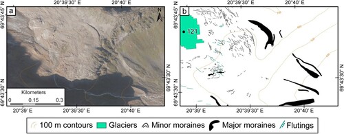
Moraines are subdivided into two categories based upon size. Major moraines, either formed of one large feature or a composite formed by the superimposition of multiple moraine crests, have been mapped as polygons, with the boundaries drawn around the proximal and distal slopes (Figure 2). Minor moraines (e.g. those <4 m wide), mostly found within likely Little Ice Age glacier limits (see Leigh et al., 2020), are mapped as lines which are drawn along their crests (Figure 2).

4.2. Ridges within areas of discrete debris accumulations (DDA)

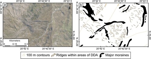
We define small areas (generally <0.2 km²) of complex, hummocky ridge systems as ‘ridges within areas of discrete debris accumulations’ (DDA; sensu Whalley, 2009, 2012). DDA as described by Whalley (2012) is ‘a non-genetic and descriptive term ... without any preconceived notion of origin’ (Whalley, 2012, p. 3). These features appear as a complex and often disorganised network of ridges and furrows separated by a mix of sediment veneer, boulders, and vegetated ground (Figure 3). Ridge crest patterns display no dominant orientation, and ridges are of variable lengths but not exceeding 100 m. Importantly, these DDA ridges differ from moraine ridges because they are short and discontinuous and do not appear to demarcate a clear former ice-margin. Patches of similarly complex ridge systems can be found across the region where they are contained within large latero-frontal moraines.

Figure 3. Ridges within areas of DDA lying inside and abutted up against major moraines: (a) image from norgeibilder.no (24/08/2016), (b) subset of resulting map (presented at 1:4,000 scale). When mapped, these ridges (grey lines) generally show no dominant pattern of orientation. Approximate image location: 69°42′4.18″N, 20°42′21.55″E.

4.3. Flutings

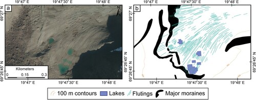
Flutings are closely spaced ridges of sediment aligned parallel to the direction of ice movement and often lying down glacier of embedded boulders or bedrock outcrops (Figure 4; e.g. Hoppe & Schytt, 1953; Boulton, 1976; Gordon et al., 1992; Benn, 1994; Evans et al., 2010). The close grouping of flutings forms a notable ridge and furrow appearance on till covered glacier forelands, aligned at right angles to individual moraines and thereby forming inset arcuate zones separated by moraines and displaying slightly offset alignments (e.g. Figure 4). Given their small size, flutings are only visible on the high-resolution orthophotographs and have been mapped as lines.

Figure 4. Flutings on the recently deglaciated foreland of glacier ID 288, showing slight variation in alignment but joining moraine ridges at right angles: (a) image from norgeibilder.no (24/08/2016), (b) subset of resulting map (presented at 1:4,000 scale). Approximate image location: 69°26′54.06″N, 19°47′27.69″E.

4.4. Eskers

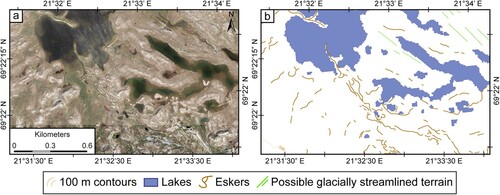
A series of distinctive ridges, predominantly in the south-east of the region, have been mapped as eskers. Classification is based on their sinuous planform; extensive length (with consideration of post depositional fragmentation); orientation parallel to sub-parallel with presumed ice flow direction; and oblique to features identified as end moraines (e.g. Brennand, 2000; Delaney, 2002; Price, 1966, 1969; Shilts et al., 1987; Storrar et al., 2014, 2015, 2020; Warren & Ashley, 1994). They also appear as lighter-coloured landscape features due to the higher proportion of glaciofluvial material (e.g. sand: Storrar & Livingstone, 2017). Eskers mostly comprise multiple ridges forming integrated networks but can occasionally occur as isolated features (Figure 5).

Figure 5. A series of eskers in an area of subdued topography in the plateau region of central Troms and Finnmark: (a) image from norgeibilder.no (24/08/2016), (b) subset of resulting map (presented at 1:8000 scale). The eskers comprise a simple, linear configuration in the north and a more complex network diverging into multiple flow directions in the east, south east, and south. Approximate image location: 69°22′6.80″N, 21°32′48.49″E.

Two panels; the left panel shows an orthophotograph of an upland area with a series of large lakes and dissected eskers, the right panel shows a geomorphological map of the same area at the same scale.

4.5. Irregular mounded terrain

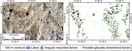
Irregular mounded terrain comprises series of low relief, disorganised, and irregular mounds, in places intersected by interweaving meltwater channels and small ponds (generally <2000 m², possibly kettle holes; Figure 6). This type of terrain broadly occurs as bands ∼0.4 km wide and is found only in the south-eastern part of the continental plateau area, near large esker networks. Mapping of individual mounds as polygon features has revealed no pattern to their orientation and shows individual mounds can vary in form from small, simple mounds of ∼25 m² to larger, branched ridges of ∼3100 m² (Figure 6). Occasional strips of coarse, bouldery and unvegetated debris occur between mounds. These mounds have a distinctly different morphology to the ridges classified as moraines and eskers and, to ensure clarity, we do not classify these landforms. Indeed, the origin of the features is unclear, although a likely genesis could include the incision of meltwater into a thick till cover, the dissection and reworking of extensive and complex esker networks, or the differential melting of highly debris covered glacier ice during the final stages of ice-sheet deglaciation in the region.

Figure 6. Three swaths of irregular mounded terrain formed in parallel with each other in an area of subdued topography in the plateau region of central Troms and Finnmark: (a) image from norgeibilder.no (24/08/2016), (b) subset of resulting map (presented at 1:8000 scale). The mounds show no dominant shape or orientation but form bands (≤ 500 m wide) of densely spaced mounds. Approximate image location: 69°20′44.79″N, 21°33′27.13″E.

Two panels; the left panel shows an orthophotograph of an upland area with a collection of irregularly shaped mounds clustered in three swaths in parallel with each other, the right panel shows a geomorphological map of the same area at the same scale.

4.6. Glacial lineations

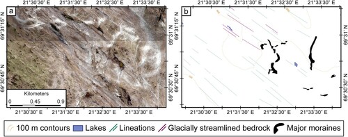
Glacial lineations are large, straight-crested landforms composed of sediment aligned parallel to the direction of former ice flow and sometimes differentiated as drumlins or mega-scale glacial lineations, with the latter exhibiting much greater length and higher elongation ratios (e.g. Clark, 1993, 1997; Stokes et al., 2013; Stokes & Clark, 2003). Those mapped in this study resemble drumlins and most occur within Reisadalen, a ∼3.5 km wide U-shaped valley in the central part of the study area, and on the southwest Finnmark plateau. The lineations are up to 1.4 km long and have been mapped as lines drawn along their crests. Lineations occur near glacially streamlined bedrock features (see Section 4.7) with which they are aligned (e.g. Figure 7).

Figure 7. Glacial lineations and associated glacially streamlined bedrock, locally overlain by moraines, and recording a former north-westerly ice flow direction: (a) image from norgeibilder.no (24/08/2016), (b) subset of resulting map (presented at 1:12,000 scale). Approximate image location: 69°30′48.99″N, 21°32′11.01″E.

Two panels; the left panel shows an orthophotograph of an upland area characterised by linear features (streamlined bedrock and lineations; NW orientation) and moraines, the right panel shows a geomorphological map of the same area at the same scale.

4.7. Glacially streamlined bedrock

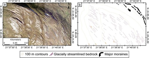
The term ‘glacially streamlined bedrock’ is used to describe an assortment of (near-) linear landforms composed of bedrock and aligned parallel with the direction of former ice flow, which are mapped as lines. Glacially streamlined bedrock occurs at both small and large scale, metres to hundreds of metres in length and up to several metres in height and width (Figure 8). It is important to note that there is potential for identification errors in cases where bedrock structure is aligned closely parallel to streamlined features (cf. Darvill et al., 2014; Lovell et al., 2011), although ice scouring is known to accentuate structural ridges (cf. Bradwell et al., 2008; Krabbendam & Bradwell, 2011; Livingstone et al., 2010; Newton et al., 2018).

Figure 8. Glacially streamlined bedrock developed across an upland flanked by two glacial valleys: (a) image from norgeibilder.no (24/08/2016), (b) subset of resulting map (presented at 1:12,000 scale). The streamlining gently curves from a mean direction of 334° in the south-east to a mean direction of 300° in the north-west and parallels the orientation of the valleys on either side. Approximate image location: 69°48′9.30″N, 21°38′11.01″E.

Two panels; the left panel shows an orthophotograph of a valley side covered by exposed and streamlined bedrock (NW orientation) and moraines at the edge of the valley floor, the right panel shows a geomorphological map of the same area at the same scale.

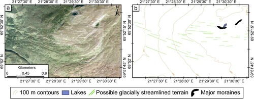
4.8. Possible glacially streamlined terrain

Throughout the study area there are areas of subdued streamlined terrain, faintly visible on the aerial imagery as series of linear features largely aligned and with a similar orientation (Figure 9). These features are often not discernible on the DEM and, as such, it is therefore difficult to interpret their true form. We have, however, mapped them as linear features, under the classification of ‘possible glacially streamlined terrain’ and, where mapped, their orientation matches that of other nearby streamlined features (e.g. glacially streamlined bedrock). Caution is, however, advised before any specific interpretation of these features is made, which would clearly benefit from fieldwork e.g. to examine possible striae and/or abrasion surfaces, etc.

Figure 9. An example of some linear features mapped as possible glacially streamlined terrain: (a) image from norgeibilder.no (24/08/2016), (b) subset of resulting map (presented at 1:12,000 scale). While there appears to be some semblance of ridges aligned parallel to each other and with a similar orientation, they are subdued to the extent they are not all discernible on the DEM. Approximate image location: 69°52′26.50″N, 21°29′48.77″E.

Two panels; the left panel shows an orthophotograph of a valley side with evidence of possible streamlining of the terrain (W and NWW orientation), the right panel shows a geomorphological map of the same area at the same scale.

4.9. Pronival ramparts

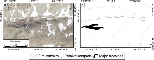
Pronival ramparts (formerly/alternatively protalus ramparts; Hedding, 2011) are distinctive ridges of open blockwork, formed beneath bedrock cliffs and talus slopes at the downslope margins of past and/or present perennial or semi-permanent snow-patches (e.g. Figure. 10). They can appear similar in form to moraine ridges but generally have a ridge crest to talus-foot distance of <70 m and there are no glacial erosional forms or evidence of over-deepening of the associated upslope areas. Their widths can vary, and individual ridges can be partially superimposed, but their length is generally <500 m (Ballantyne & Benn, 1994; Hedding, 2016; Hedding & Sumner, 2013; Shakesby, 1997). Active features have a snow-patch occupying their proximal faces. On the high-resolution orthophotographs it is possible to identify the ridges as formed of angular (blocky) debris with little to no soil/vegetation cover on their sides/crest. Pronival ramparts have been mapped as lines drawn along the crest of each individual ridge (Figure 10).

Figure 10. A row of individual pronival ramparts: (a) image from norgeibilder.no (24/08/2016), (b) subset of resulting map (presented at 1:4000 scale). The ramparts sit at the foot of a talus slope, below a valley rock wall that contains several very small (<0.01 km²) perennial snow patches. There is a lateral moraine to the left of the image, lying distal to the pronival ramparts, indicative of the sequential development of inset parallel ridges of different origins during overall deglaciation of the valley. Approximate image location: 69°51′39.07″N, 20°16′19.02″E.

Two panels; the left panel shows an orthophotograph of valley sidewall with pronival ramparts formed at the base of the valley wall and a moraine distal to the rampart, the right panel shows a geomorphological map of the same area at the same scale.

4.10. Rock glaciers and glacierised landforms

Rock glaciers are identifiable as lobate, ridged masses of angular debris that resemble small glaciers, and are moving or have moved downslope due to the deformation of internal ice lenses or frozen sediments. They may also form from downwasting debris-covered mountain glaciers, although the definition of rock glaciers using genetic versus descriptive criteria is a contentious issue (cf. Barsch, 1996; Benn et al., 2003; Berthling, 2011; Hamilton & Whalley, 1995; Hedding, 2016; Whalley et al., 1995; Whalley & Martin, 1992). Smaller lobate, ridged masses can also be developed by the process of rock glacierisation of existing landforms, such as moraines or protalus ridges (e.g. England, 1978; Evans, 1993; Matthews et al., 2017; Matthews & Petch, 1982; Thompson, 1954). We avoid inferring formation mechanisms and adopt a purely descriptive approach to mapping rock glaciers, following the protocols used by Dyke et al. (1982) and Evans et al. (2006, 2016a, 2016b) in mapping landforms in glacierised mountains. A pronounced convex morphology of individual lobes is indicative of an active ice core, while a less distinct, flat or collapsed appearance indicates older/relict lobes with a melting/melted ice core (inactive or relict: Ikeda & Matsuoka, 2002; Sattler et al., 2016); although in most cases the margins of rock glaciers remain identifiable by steep front and side slopes (e.g. 26–36°; Lindner & Marks, 1985). The rock glaciers we mapped may or may not have a present-day ice core, although this is often not a characteristic that can be immediately determined (cf. Whalley, 2020). We have, therefore, not attempted to quantify ice presence in our classifications. These accumulations of rock debris generally, but not exclusively, have lengths greater than their widths and are immediately recognisable by their bouldery surface of (superimposed) ridges and furrows (Ballantyne & Harris, 1994; Ballantyne & Kirkbride, 1986; Hamilton & Whalley, 1995; Lilleøren & Etzelmüller, 2011). Large rock glaciers can be identified on all imagery types and the ridge structures can be interpreted on the DEM where the elevation difference between ridges is >2 m. Many smaller rock glaciers, however, need to be viewed on the orthophotographs to enable identification of individual ridges within the main landform assemblage. All rock glaciers are depicted by polygons representing their outer margins inset with lines drawn along ridge/lobe crests.

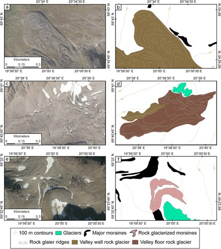
Notwithstanding the ongoing debate surrounding rock glacier origins and classifications (see Berthling, 2011 and references therein), we categorise rock glaciers as either ‘valley floor rock glaciers’ or ‘valley wall rock glaciers’. We define valley wall rock glaciers (including protalus lobes e.g. ridges at the foot of talus slopes meeting the criteria of a pronival rampart but showing evidence of flow; Blagborough & Breed, 1967; Chattopadhyay, 1984; Gray, 1970; Johnson et al., 2007; Matthews et al., 2017; Millar & Westfall, 2008; Wilson, 1990) as rock glaciers that appear to have formed independently of glacier ice cores, and presumed to have formed as the result of creep of rock slope failure (RSF) or talus deposits (Figure 11(a,b)). Indeed, protalus lobes evidence the early stages of gravitationally induced deformation of interstitial ice (Lindner & Marks, 1985; Matthews et al., 2013), representing the embryonic form of a rock glacier, a key component in the rock glacier continuum (e.g. Hedding, 2011; Sattler et al., 2016; Serrano & López-Martı́nez, 2000). We define valley floor rock glaciers as features that have clearly evolved at the margins of former debris-charged glaciers, for example, those that occur at the foot of a glacial cirque (Figure 11(c,d)). The example of a valley floor rock glacier in Figure 11(c,d) has clearly defined ridges within the rock debris, fills a substantial portion of the cirque, and extends up to the 2018 glacier margin. Figure 11(c,d) also shows a valley wall rock glacier that is distinctly separate from that of the main rock glacier on the cirque floor. These two rock glaciers (Figure 11(c,d)) could, over time, effectively fuse together to form a large complex landform, from which it might not be possible to define separate origins. The ability to identify and map each individual landforms (valley wall and valley floor rock glaciers) at the present day, therefore, provides a unique insight into rock glacier equifinality and the evidence of periglacial processes working in this highly active region.

Figure 11. A collection of rock glacierised landforms: (a, b) A large valley wall rock glacier with a clear lobate form, multiple (sometimes bifurcating) surface ridges, and convex profile. (c, d) A large valley floor rock glacier showing multiple, overlapping lobes, formed beneath a very small glacier (not included in the 2012 Inventory of Norwegian Glaciers), and connected to a small valley wall rock glacier on its northern margin. (e,f) Rock glacierised frontal portions of a latero-frontal moraine fronting a small glacier (not included in the 2012 Inventory of Norwegian Glaciers). The rock glacierised section of the moraine is inset with smaller ridges and furrows indicative of post-depositional modification of a glacial ice core. All images from norgeibilder.no (24/08/2016) and map subsets at 1:4,000 scale, with glaciers mapped on 2018 satellite imagery. Approximate image locations: 69°42′57.27″N, 20°33′54.42″E; 69°40′50.97″N, 20°38′24.74″E; 69°32′46.83″N, 19°59′55.71″E.

Six panels in two columns; the left panels show orthophotographs of different rock glaciers and rock glacierised moraines, the right panels show geomorphological maps of the same area at the same scale.

Finally, we separately define and map ‘rock glacierized moraines’ on the basis that these moraines display discrete evidence of localised periglacial downslope deformation (cf. England, 1978; Østrem, 1964; Thompson, 1957; Whalley, 2009). This moraine deformation manifests as part of a moraine transforming from a largely linear or curvilinear feature, such as a lateral or frontal moraine, into a lobate ridged or spatulate form (Figure 11(e,f)). Such moraines may be accompanied by areas of debris within their proximal margins that appear to be deforming either due to permafrost creep of interstitial ice and/or deformation of a buried glacial ice core. The term ‘rock glacierized’ is not strictly genetic, but simply refers to parts of moraines that have been developed into rock glaciers. Rock glacierised moraines are generally found within smaller valleys and are mapped as polygons, with the boundaries drawn around the proximal and distal slopes.

4.11. Lithalsas

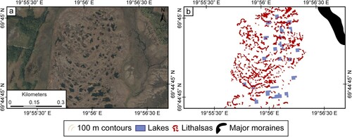
Lithalsas (or ‘mineral palsas’) are vegetation-free frost-heaved permafrost mounds (showing little pattern in their formation) rising out of a bog/mire (Harris, 1993; Ballantyne, 2018; Figure 12). They can develop into mounds up to ∼8 m high with diameters of ∼120 m (Pissart et al., 2011; Wolfe et al., 2014). Lithalsas are formed on frost-susceptible substrates including till, alluvium, lake, and marine deposits with high ground water availability (Ballantyne, 2018). Throughout the study site lithalsas were only identified and mapped on the western side of the Lyngen peninsula, outside the mapped valley moraine limits, and in areas not exceeding 20 m a.s.l. Given their small size, lithalsas are only visible on the high-resolution orthophotographs and have been mapped as polygons.

Figure 12. An area of lithalsas at low level and distal to the valley moraine system: (a) image from norgeibilder.no (24/08/2016), (b) subset of resulting map (presented at 1:4,000 scale). The lithalsas are neatly constrained to the wetland area formed from a light-coloured sediment like that of glaciofluvial sediments seen elsewhere in the region. Note however, that most of the closely situated lakes in this wetland are too small to be mapped from satellite imagery and hence are not shown on this map. Approximate image location: 69°44′43.95″N, 19°55′53.87 ″E.

Two panels; the left panel shows an orthophotograph of a lowland area with lithalsas and small lakes, the right panel shows a geomorphological map of the same area at the same scale.

4.12. Contemporary glaciers and lakes

Mapping of glacier outlines was guided by the prior outlines of Andreassen et al. (2012) and Leigh et al. (2020). Glaciers are easily identifiable on the multispectral imagery, especially when using a false colour composite of bands 5-4-3 as Red–Green–Blue, whereby glaciers appear as bright, fluorescent blue (e.g. Andreassen et al., 2012; Raup et al., 2007). Lakes and smaller inland waterbodies are found localised in a basin or constrained by other geomorphological features (e.g. moraines) and are easily identifiable on the multispectral imagery using both true and false colour composites. As the extent of lakes is seasonally variable, the size of mapped polygons is dependent on image capture date. Both glaciers and lakes were mapped as polygons, with the lines drawn around their margins.

A total of 404 glaciers and 3041 lakes were mapped and these range in size from 0.01 to 8.15 km² for glaciers and 400 m² (0.0004 km²) to 10 km² for lakes. Around 84% of all mapped glaciers are in the central and western area and around 41% of lakes are in the south-east of the study area. At the time of image capture (2018/19), we identify 36 ice-contact proglacial lakes (≥0.0004 km²), of which 53% are on the Lyngen Peninsula.

5. Summary and conclusions

This paper presents a new glacial and periglacial geomorphological map of a ∼6800 km² region of central Troms and Finnmark county, northern Norway (Man Map). The map reveals complex suites of landform assemblages that include previously unmapped components of the geomorphological record pertaining to the interaction of glacial and periglacial regimes in mountainous terrain. Our mapping also revises and updates the older and more generic superficial geology mapping of the central Troms and Finnmark region (e.g. Bergstrøm & Neeb, 1984; Sveian et al., 2005; Tolgensbakk & Og Sollid, 1988 etc.), most notably by mapping: (1) previously un-mapped and recently deglaciated terrain (up to the 2016 glacier margins, and including the 2018/19 glacier extent), enabling the documentation of small and often poorly-preserved geomorphological features present in these active environments (e.g. annual moraines, flutings, ice-contact proglacial lakes etc.); and (2) individual moraine ridges (with no minimum size-threshold), enabling the identification of closely spaced and occasionally bifurcating moraine ridges indicative of minor fluctuations of glacier margins and these were found at valley heads, within valleys, and at active glacier margins.

Additionally, we note that throughout our study area, and especially across the Lyngen Peninsula, very small glaciers (<0.05 km²) have supraglacial debris cover at/around their fronts. The debris cover often masks the boundaries of the glaciers, making it difficult to map the full extent of the ice, especially using satellite imagery. This indicates that buried (stagnant) glacier ice is widespread on the heavily debris covered forelands fronting cirque glaciers, which has implications for the development of glacier-derived rock glaciers and rock glacierised moraines. Indeed, Griffey and Whalley (1979) previously noted that it is likely that large rock avalanches supplied the small glaciers 187 and 188 with an abnormally large quantity of debris, leading to the development of the rock glacier in the area.

Of particular interest for future glacial geochronological studies are the extensive moraine systems that are mapped throughout the region, covering a total area of ∼63.7 km². Large terminal and recessional moraine complexes are mainly located at the heads of and within mountain valleys and were likely formed during the retreat of the Scandinavian Ice Sheet at the termination of the Younger Dryas or several episodes of glacial advance or still-stands throughout the Holocene. The distribution of glacial valleys near the fjord systems, and the complex moraine systems they contain, indicate that the maritime mountain regions of Troms and Finnmark County experienced extensive alpine-style glaciations (Neoglacial Events; Matthews & Briffa, 2005; Matthews & Dresser, 2008; Nesje & Kvamme, 1991; Wanner et al., 2011 etc.), with evidence of ice caps and ice field glaciation limited to and centred on the higher plateaux areas further inland and towards the Norwegian boarder (cf. Evans et al., 2002).

There is a notable decrease in the prevalence of landforms within the glacial/periglacial domain across a west to east transect. The alpine terrain that characterises the central/western side of the study area (e.g. the Lyngen Peninsula, Nordreisa and Kåfjord municipalities, and the islands of Uløya and Kågen) has a high volume of glacial and periglacial landforms. In contrast, the broad valleys, plateaux regions, and smaller mountain belts that characterise the eastern/south-eastern side of our study area have fewer mountain glaciers and, where ice is present, it is more commonly in the form of plateau glaciers covering areas of subdued topography. The distribution of mapped landforms can be attributed not only to the terrain, but also likely reflects the substantial precipitation gradient that is present across our study area from west to east.

The prevalence of permafrost across large areas of land throughoutour study area has resulted in a wide variety of periglacial phenomena, much of which remains outside the scope of our mapping. The most notable features are those associated with seasonally frozen ground (e.g. patterned ground) and mass wasting (e.g. gelifluction). In areas of complex glacial geomorphology extensive periglacial mass wasting can not only alter the appearance and structure of glacial landforms (e.g. rock glacierised moraines; see Section 4.11) but can also, mask or subdue the presence, and/or imitate the form, of glacial features. Greater care must, therefore, be taken when mapping the small-scale glacial geomorphological features in areas of active periglacial processes.

The map resulting from this work further demonstrates the utility of high-resolution aerial imagery and DEMs (e.g. <1 m orthophotographs, 2 m Arctic DEM), combined with medium-resolution satellite imagery (e.g. 10 m Sentinel-2A/2B), and their associated remote sensing techniques, for mapping glacial and periglacial geomorphology across large swaths of rugged and poorly accessible terrain. Our map can be used to underpin robust palaeoglaciological reconstructions of plateau and mountain glaciers, enable new interpretations of mountain glacier dynamics in a highly sensitive Arctic region, further refining existing models of mountain glacial landsystems, and can help guide future field investigations throughout the region.

Software

Features were identified and digitally mapped as either vector lines or polygons using ESRIs ArcGIS software (version 10.5.1) and a projected coordinate system of WGS_1984_UTM_Zone_33N. Final map/figure production was undertaken in Adobe Illustrator CS6.

Data used in the production of the accompanying map is supplied as supplementary material (as ESRI Shapefiles). The data are supplied for use but must be cited as per this article and remain the copyright of the author (Leigh, J.R.). Each landform has specific attributes, the attributes are listed as follows with the shapefile attribute column titles shown within brackets: (i) Shape type (Shape); (ii) Object name (Object_Nam); (iii) Shape area (Shape_Area); (iv) Shape length (Shape_Leng); (v) Data source (Data_Src); (vi) Image type (Imag_Type); (vii) Image resolution (Imag_Res); (viii) Image date (Imag_Date); (ix) Measurement method (Meas_Meth); (x) Loose mass type (Jordart*); (xi) Material description (Mat_Desc); (xii) Feature location on earth surface (Medium*); (xiii) Analyst Forename (Anlst_For); (xiv) Analyst Surname (Anlst_Sur); (xv) Mapping date (Map_Date). Where relevant (as denoted by the *) shapefile attributes have been coded following the Norwegian Geological Surveys (NGU) product specification for ‘loose materials, version 3.0’ (NGU, 2015) in line with Norwegian, Systematic Organization of Spatial Information (SOSI) codes.

Acknowledgements

This work would not have been possible without the digital archive of high-resolution aerial imagery provided by www.norgeibilder.no which is a cooperation between the Norwegian Public Roads Administration, the Norwegian Institute of Bioeconomics (NIBIO), and the Norwegian Mapping Authority (Kartverket). The high-resolution Arctic DEMs were provided by the Polar Geospatial Center under NSF-OPP awards 1043681, 1559691, and 1542736. We also thank ESA and USGS for providing free satellite imagery and the Geological Survey of Norway (NGU) for providing freely available geological data (made available by the Norwegian license for public data; NLOD). We thank the editors (Mike Smith and Martin Margold) and are grateful for the diligent reviews of Brian Whalley, Jostein Bakke, and Heike Apps, who provided valuable comments and insight which improved the quality and clarity of the map and accompanying manuscript. Joshua R. Leigh is supported by the Natural Environment Research Council UK studentship, reference: NE/L002590/1.

Disclosure statement

No potential conflict of interest was reported by the author(s).

Additional information

Funding

This work was supported by Natural Environment Research Council [grant number NE/L002590/1].

References

- Aitkenhead, N. (1960). Observations on the drainage of a glacier-dammed lake in Norway. Journal of Glaciology, 3(27), 607–611. https://doi.org/https://doi.org/10.1017/S0022143000023728
- Andersen, B. (1968). Glacial Geology of western Troms, north Norway. Norges Geologiske Undersøkelse, 256, 1–160.
- Andreassen, L. M., Winsvold, S. H., Paul, F., & Hausberg, J. E. (2012). Inventory of Norwegian glaciers. In L. M. Andreassen & S. H. Winsvold (Eds.), 1–236. Norwegian Water Resources and Energy Directorate.
- Arenson, L. U., & Jakob, M. (2015). Periglacial geohazard risks and ground temperature increases. In G. Lollino, A. Manconi, J. Clague, W. Shan, & M. Chiarle (Eds.), Engineering Geology for Society and territory - volume 1 (pp. 233–237). Springer.
- Bakke, J., Dahl, S. O., Paasche, Ø, Løvlie, R., & Nesje, A. (2005). Glacier fluctuations, equilibrium-line altitudes and Palaeoclimate in Lyngen, northern Norway, during the Lateglacial and Holocene. The Holocene, 15(4), 518–540. https://doi.org/https://doi.org/10.1191/0959683605hl815rp
- Ballantyne, C. K. (1990). The Holocene glacial history of Lyngshalvøya, northern Norway: Chronology and climatic implications. Boreas, 19(2), 93–117. https://doi.org/https://doi.org/10.1111/j.1502-3885.1990.tb00570.x
- Ballantyne, C. K. (2018). Periglacial geomorphology. John Wiley and Sons.
- Ballantyne, C. K., & Benn, D. I. (1994). Glaciological constraints on Protalus rampart development. Permafrost and Periglacial Processes, 5(3), 145–153. https://doi.org/https://doi.org/10.1002/ppp.3430050304
- Ballantyne, C. K., & Harris, C. (1994). The periglaciation of Great Britain. Cambridge University Press.
- Ballantyne, C. K., & Kirkbride, M. P. (1986). The characteristics and significance of some Lateglacial protalus ram parts in upland Britain. Earth Surface Processes and Landforms, 11(6), 659–671. https://doi.org/https://doi.org/10.1002/esp.3290110609
- Barsch, D. (1996). Rockglaciers: Indicators for the present and former Geoecology in high mountain environments. Springer Science & Business Media.
- Benn, D. I. (1994). Fluted moraine formation and till genesis below a temperate valley glacier: Slettmarkbreen, jotunheimen, southern Norway. Sedimentology, 41(2), 279–292. https://doi.org/https://doi.org/10.1111/j.1365-3091.1994.tb01406.x
- Benn, D. I., & Evans, D. J. A. (2010). Glaciers and glaciation (2nd ed). Routledge.
- Benn, D. I., Kirkbride, M. P., Owen, L. A., & Brazier, V. (2003). Glaciated valley landsystems. In D. J. A. Evans (Ed.), Glacial landsystems (pp. 372–406). Arnold.
- Bergstrøm, B., & Neeb, P. R. (1984). Resiadalen. Beskrivelse til kvartaergologisk kart 1734 III, M 1:50,000 (med fargetrykt kart). Norges Geologiske Undersøkelse.
- Berthling, I. (2011). Beyond confusion: Rock glaciers as cryo-conditioned landforms. Geomorphology, 131(3–4), 98–106. https://doi.org/https://doi.org/10.1016/j.geomorph.2011.05.002
- Bickerdike, H. L., Ó Cofaigh, C., Evans, D. J. A., & Stokes, C. R. (2018). Glacial landsystems, retreat dynamics and controls on Loch Lomond Stadial (Younger Dryas) glaciation in Britain. Boreas, 47(1), 202–224. https://doi.org/https://doi.org/10.1111/bor.12259
- Blagborough, J. W., & Breed, W. J. (1967). Protalus ramparts on Navajo mountain, Utah. American Journal of Science, 265(9), 759–773. https://doi.org/https://doi.org/10.2475/ajs.265.9.759
- Boulton, G. S. (1976). The origin of glacially fluted surfaces-observations and theory. Journal of Glaciology, 17(76), 287–309. https://doi.org/https://doi.org/10.1017/S0022143000013605
- Boulton, G. S. (1986). Push-moraines and glacier-contact fans in marine and terrestrial environments. Sedimentology, 33(5), 677–698. https://doi.org/https://doi.org/10.1111/j.1365-3091.1986.tb01969.x
- Bradwell, T., Stoker, M. S., Golledge, N. R., Wilson, C. K., Merritt, J. W., Long, D., Everest, J. D., Hestvik, O. B., Stevenson, A. G., Hubbard, A. L., & Finlayson, A. G. (2008). The northern sector of the last British Ice sheet: Maximum extent and demise. Earth-Science Reviews, 88(3–4), 207–226. https://doi.org/https://doi.org/10.1016/j.earscirev.2008.01.008
- Brennand, T. A. (2000). Deglacial meltwater drainage and glaciodynamics: Inferences from Laurentide eskers, Canada. Geomorphology, 32(3–4), 263–293. https://doi.org/https://doi.org/10.1016/S0169-555X(99)00100-2
- Burki, V., Larsen, E., Fredin, O., & Margreth, A. (2009). The formation of sawtooth moraine ridges in Bødalen, western Norway. Geomorphology, 105(3–4), 182–192. https://doi.org/https://doi.org/10.1016/j.geomorph.2008.06.016
- Chandler, B. M. P., Chandler, S. J. P., Evans, D. J. A., Ewertowski, M. W., Lovell, H., Roberts, D. H., Schaefer, M., & Tomczyk, A. M. (2020). Sub-annual moraine formation at an active temperate Icelandic glacier. Earth Surface Processes and Landforms, 45(7), 1622–1643. https://doi.org/https://doi.org/10.1002/esp.4835
- Chandler, B. M. P., Evans, D. J. A., Roberts, D. H., Ewertowski, M., & Clayton, A. I. (2016). Glacial geomorphology of the Skálafellsjökull foreland, Iceland: A case study of ‘annual’ moraines. Journal of Maps, 12(5), 904–916. https://doi.org/https://doi.org/10.1080/17445647.2015.1096216
- Chandler, B. M. P., Lovell, H., Boston, C. M., Lukas, S., Barr, I. D., Benediktsson, ÍÖ, Benn, D. I., Clark, C. D., Darvill, C. M., Evans, D. J. A., & Ewertowski, M. (2018). Glacial geomorphological mapping: A review of approaches and frameworks for best practice. Earth-Science Reviews, 185, 806–846. https://doi.org/https://doi.org/10.1016/j.earscirev.2018.07.015
- Chandler, B. M. P., & Lukas, S. (2017). Reconstruction of Loch Lomond Stadial (Younger Dryas) glaciers on Ben more Coigach, NW Scotland, and implications for reconstructing palaeoclimate using small ice masses. Journal of Quaternary Science, 32(4), 475–492. https://doi.org/https://doi.org/10.1002/jqs.2941
- Chandler, B. M. P., Lukas, S., Boston, C. M., & Merritt, J. W. (2019). Glacial geomorphology of the Gaick, central Grampians, Scotland. Journal of Maps, 15(2), 60–78. https://doi.org/https://doi.org/10.1080/17445647.2018.1546235
- Chattopadhyay, G. P. (1984). A fossil valley-wall rock glacier in the cairngorm mountains. Scottish Journal of Geology, 20(1), 121–125. https://doi.org/https://doi.org/10.1144/sjg20010121
- Clark, C. D. (1993). Mega-scale glacial lineations and cross-cutting ice-flow landforms. Earth Surface Processes and Landforms, 18(1), 1–29. https://doi.org/https://doi.org/10.1002/esp.3290180102
- Clark, C. D. (1997). Reconstructing the evolutionary dynamics of former ice sheets using multi-temporal evidence, remote sensing and GIS. Quaternary Science Reviews, 16(9), 1067–1092. https://doi.org/https://doi.org/10.1016/S0277-3791(97)00037-1
- Clark, C. D., Hughes, A. L. C., Greenwood, S. L., Spagnolo, M., & Ng, F. S. L. (2009). Size and shape characteristics of drumlins, derived from a large sample, and associated scaling laws. Quaternary Science Reviews, 28(7–8), 677–692. https://doi.org/https://doi.org/10.1016/j.quascirev.2008.08.035
- Ó Cofaigh, C., Evans, D. J. A, & England, J. (2003). Ice-marginal terrestrial landsystems: Sub-polar glacier margins of the Canadian and Greenland high Arctic. In D. J. A. Evans (Ed.), Glacial landsystems (pp. 44–64). Arnold.
- Darvill, C. M., Stokes, C. R., Bentley, M. J., Evans, D. J. A., & Lovell, H. (2017). Dynamics of former ice lobes of the southernmost Patagonian Ice Sheet based on a glacial landsystems approach. Journal of Quaternary Science, 32(6), 857–876. https://doi.org/https://doi.org/10.1002/jqs.2890
- Darvill, C. M., Stokes, C. R., Bentley, M. J., & Lovell, H. (2014). A glacial geomorphological map of the southernmost ice lobes of Patagonia: The Bahía Inútil–San Sebastián, Magellan, Otway, Skyring and Río Gallegos lobes. Journal of Maps, 10(3), 500–520. https://doi.org/https://doi.org/10.1080/17445647.2014.890134
- Delaney, C. (2002). Sedimentology of a glaciofluvial landsystem, Lough Ree area, central Ireland: Implications for ice margin characteristics during Devensian deglaciation. Sedimentary Geology, 149(1–3), 111–126. https://doi.org/https://doi.org/10.1016/S0037-0738(01)00247-0
- Du, Y., Zhang, Y., Ling, F., Wang, Q., Li, W., & Li, X. (2016). Water bodies’ mapping from sentinel-2 imagery with modified normalized difference water index at 10-m spatial resolution produced by sharpening the SWIR band. Remote Sensing, 8(354), 1–19. https://doi.org/https://doi.org/10.3390/rs8040354
- Dyke, A. S., Andrews, J. T., & Miller, G. H. (1982). Quaternary Geology of Cumberland peninsula. District of Franklin. Geological Survey of Canada. Memoir 403.
- England, J. (1978). The glacial geology of northeastern Ellesmere Island, NWT, Canada. Canadian Journal of Earth Sciences, 15(4), 603–617. https://doi.org/https://doi.org/10.1139/e78-065
- Eriksen, HØ, Rouyet, L., Lauknes, T. R., Berthling, I., Isaksen, K., Hindberg, H., Larsen, Y., & Corner, G. D. (2018). Recent acceleration of a rock glacier complex, Adjet, Norway, documented by 62 years of remote sensing observations. Geophysical Research Letters, 45(16), 8314–8323. https://doi.org/https://doi.org/10.1029/2018GL077605
- Evans, D. J. A. (1993). High-latitude rock glaciers: A case study of forms and processes in the Canadian Arctic. Permafrost and Periglacial Processes, 4(1), 17–35. https://doi.org/https://doi.org/10.1002/ppp.3430040103
- Evans, D. J. A. (2001). Glaciers. Progress in Physical Geography: Earth and Environment, 27(2), 261–274. https://doi.org/https://doi.org/10.1191/0309133303pp380pr
- Evans, D. J. A., Ewertowski, M., & Orton, C. (2016a). Eiriksjökull plateau icefield landsystem, Iceland. Journal of Maps, 12(5), 747–756. https://doi.org/https://doi.org/10.1080/17445647.2015.1072448
- Evans, D. J. A., Ewertowski, M., & Orton, C. (2017a). The glaciated valley landsystem of Morsárjökull, southeast Iceland. Journal of Maps, 13(2), 909–920. https://doi.org/https://doi.org/10.1080/17445647.2017.1401491
- Evans, D. J. A., Ewertowski, M., & Orton, C. (2017b). Skaftafellsjokull, Iceland: Glacial geomorphology recording glacier recession since the Little Ice Age. Journal of Maps, 13(2), 358–368. https://doi.org/https://doi.org/10.1080/17445647.2017.1310676
- Evans, D. J. A., Ewertowski, M. W., & Orton, C. (2019). The glacial landsystem of Hoffellsjökull, SE Iceland: Contrasting geomorphological signatures of active temperate glacier recession driven by ice lobe and bed morphology. Geografiska Annaler: Series A, Physical Geography, 101(3), 249–276. https://doi.org/https://doi.org/10.1080/04353676.2019.1631608
- Evans, D. J. A., Ewertowski, M., Orton, C., & Graham, D. J. (2018). The glacial geomorphology of the Ice Cap piedmont lobe landsystem of east Mýrdalsjökull, Iceland. Geosciences, 8(6), 194. https://doi.org/https://doi.org/10.3390/geosciences8060194
- Evans, D. J. A., Ewertowski, M., Orton, C., Harris, C., & Guðmundsson, S. (2016b). Snæfellsjökull volcano-centred ice cap landsystem, west Iceland. Journal of Maps, 12(5), 1128–1137. https://doi.org/https://doi.org/10.1080/17445647.2015.1135301
- Evans, D. J. A., Nelson, C. D., & Webb, C. (2010). An assessment of fluting and “till esker” formation on the foreland of Sandfellsjökull. Iceland. Geomorphology, 114(3), 453–465. https://doi.org/https://doi.org/10.1016/j.geomorph.2009.08.016
- Evans, D. J. A., Rea, B. R., Hansom, J. D., & Whalley, W. B. (2002). Geomorphology and style of plateau icefield deglaciation in fjord terrains: The example of Troms-Finnmark, north Norway. Journal of Quaternary Science, 17(3), 221–239. https://doi.org/https://doi.org/10.1002/jqs.675
- Evans, D. J. A., & Twigg, D. R. (2002). The active temperate glacial landsystem: A model based on Breiðamerkurjökull and Fjallsjökull, Iceland. Quaternary Science Reviews, 21(20–22), 2143–2177. https://doi.org/https://doi.org/10.1016/S0277-3791(02)00019-7
- Evans, D. J. A., Twigg, D. R., & Shand, M. (2006). Surficial geology and geomorphology of the Þórisjökull plateau icefield, west-central Iceland. Journal of Maps, 2006(1), 17–29. https://doi.org/https://doi.org/10.4113/jom.2006.52
- Gisnås, K., Etzelmüller, B., Lussana, C., Hjort, J., Sannel, A. B. K., Isaksen, K., Westermann, S., Kuhry, P., Christiansen, H. H., Frampton, A., & Åkerman, J. (2017). Permafrost map for Norway, Sweden and Finland. Permafrost and Periglacial Processes, 28(2), 359–378. https://doi.org/https://doi.org/10.1002/ppp.1922
- Gordon, J. E., Whalley, W. B., Gellatly, A. F., & Vere, D. M. (1992). The formation of glacial flutes: Assessment of models with evidence from Lyngsdalen, north Norway. Quaternary Science Reviews, 11(7–8), 709–731. https://doi.org/https://doi.org/10.1016/0277-3791(92)90079-N
- Gray, J. T. (1970). Mass wasting studies in the Ogilvie and Wernecke mountains, central Yukon territory. Geological Survey Canada Papers, 70, 192–195.
- Greig, D. (2011). Moraine chronology and deglaciation of the northern Lyngen Peninsula, Troms, Norway [Unpublished Master’s Thesis]. UiT The Arctic University of Norway, Tromsø.
- Griffey, N. J., & Whalley, W. B. (1979). A rock glacier and moraine–ridge complex, Lyngen Peninsula, north Norway. Norsk Geografisk Tidsskrift, 33(3), 117–124. https://doi.org/https://doi.org/10.1080/00291957908552049
- Grønlie, O. T. (1931). Breer i balsfjorden. Norsk Geografisk Tidsskrift, 12, 265–289.
- Hamilton, S. J., & Whalley, W. B. (1995). Rock glacier nomenclature: A re-assessment. Geomorphology, 14(1), 73–80. https://doi.org/https://doi.org/10.1016/0169-555X(95)00036-5
- Harris, S. A. (1993). Palsa-like mounds in a mineral substrate, Fox Lake Yukon Territory. Proceedings of the 6th International Conference on Permafrost, South China University Press, Wushan Guangzhou, pp. 238–243.
- Hättestrand, C., & Clark, C. D. (2006). The glacial geomorphology of Kola Peninsula and adjacent areas in the Murmansk region, Russia. Journal of Maps, 2(1), 30–42. https://doi.org/https://doi.org/10.4113/jom.2006.41
- Hedding, D. W. (2011). Pronival rampart and protalus rampart: A review of terminology. Journal of Glaciology, 57(206), 1179–1180. https://doi.org/https://doi.org/10.3189/002214311798843241
- Hedding, D. W. (2016). Pronival ramparts: Origin and development of terminology. Erdkunde, 70(2), 141–151. https://doi.org/https://doi.org/10.3112/erdkunde.2016.02.03
- Hedding, D. W., & Sumner, P. D. (2013). Diagnostic criteria for pronival ramparts: Site, morphological and sedimentological characteristics. Geografiska Annaler: Series A, Physical Geography, 95(4), 315–322. https://doi.org/https://doi.org/10.1111/geoa.12021
- Helland, A. (1899). Tromsø Amt I. In: Geologi. Norges Land og Folk. Aschehoug. Kristiania.
- Hjort, J., Karjalainen, O., Aalto, J., Westermann, S., Romanovsky, V. E., Nelson, F. E., Etzelmüller, B., & Luoto, M. (2018). Degrading permafrost puts Arctic infrastructure at risk by mid-century. Nature Communications, 9(1), 1–9. https://doi.org/https://doi.org/10.1038/s41467-018-07557-4
- Holmes, G. W., & Andersen, B. G. (1964). Glacial chronology of Ullsfjord, northern Norway. United States Geological Survey Professional Paper, 4750, 159–163.
- Hoppe, G., & Schytt, V. (1953). Some observations on fluted moraine surfaces. Geografiska Annaler, 35(2), 105–115. https://doi.org/https://doi.org/10.1080/20014422.1953.11880852
- Huggel, C., Allen, S., Deline, P., Fischer, L., Noetzli, J., & Ravanel, L. (2012). Ice thawing, mountains falling—are alpine rock slope failures increasing? Geology Today, 28(3), 98–104. https://doi.org/https://doi.org/10.1111/j.1365-2451.2012.00836.x
- Hughes, A. L., Gyllencreutz, R., Lohne, ØS, Mangerud, J., & Svendsen, J. I. (2016). The last Eurasian ice sheets–a chronological database and time-slice reconstruction, DATED-1. Boreas, 45(1), 1–45. https://doi.org/https://doi.org/10.1111/bor.12142
- Ikeda, A., & Matsuoka, N. (2002). Degradation of talus-derived rock glaciers in the upper Engadin. Swiss Alps. Permafrost and Periglacial Processes, 13(2), 145–161. https://doi.org/https://doi.org/10.1002/ppp.413
- IPCC (Intergovernmental Panel on Climate Change). (2019). Special report: The ocean and cryosphere in a changing climate. https://www.ipcc.ch/report/srocc/
- Jaskólski, M. W., Pawłowski, L., & Strzelecki, M. C. (2017). Assesment of geohazardsand coastal change in abandoned Arctic town, Pyramiden, Svalbard. In G. Rachlewicz (Ed.), Cryosphere reactions against the background of environmental changes in contrasting high-Arctic conditions in Svalbard. Institute of Geoecology and geoinformation A. Mickiewicz University in Poznań Polar reports, (Vol. 2 pp. 51–64). Bogucki Wydawnictwo Naukowe.
- Johnson, B. G., Thackray, G. D., & Van Kirk, R. (2007). The effect of topography, latitude, and lithology on rock glacier distribution in the Lemhi Range, central Idaho. USA. Geomorphology, 91(1–2), 38–50. https://doi.org/https://doi.org/10.1016/j.geomorph.2007.01.023
- Krabbendam, M., & Bradwell, T. (2011). Lateral plucking as a mechanism for elongate erosional glacial bedforms: Explaining megagrooves in Britain and Canada. Earth Surface Processes and Landforms, 36(10), 1335–1349. https://doi.org/https://doi.org/10.1002/esp.2157
- Leigh, J. R., Stokes, C. R., Carr, R. J., Evans, I. S., Andreassen, L. M., & Evans, D. J. A. (2019). Identifying and mapping very small ( < 0.5 km 2) mountain glaciers on coarse to high-resolution imagery. Journal of Glaciology, 65(254), 873–888. https://doi.org/https://doi.org/10.1017/jog.2019.50
- Leigh, J. R., Stokes, C. R., Evans, D. J. A., Carr, R. J., & Andreassen, L. M. (2020). Timing of Little Ice Age maxima and subsequent glacier retreat in northern Troms and western Finnmark, northern Norway. Arctic, Antarctic, and Alpine Research, 52(1), 281–311. https://doi.org/https://doi.org/10.1080/15230430.2020.1765520
- Liestøl, O. (1956). Glacier dammed lakes in Norway. Norsk Geografisk Tidsskrift, 15(3-4), 122–149. https://doi.org/https://doi.org/10.1080/00291955608542772
- Lilleøren, K. S., & Etzelmüller, B. (2011). A regional inventory of rock glaciers and ice-cored moraines in Norway. Geografiska Annaler: Series A, Physical Geography, 93(3), 175–191. https://doi.org/https://doi.org/10.1111/j.1468-0459.2011.00430.x
- Lindner, L., & Marks, L. (1985). Types of debris slope accumulations and rock glaciers in south Spitsbergen. Boreas, 14(2), 139–153. https://doi.org/https://doi.org/10.1111/j.1502-3885.1985.tb00907.x
- Livingstone, S. J., Ó. Cofaigh, C., & Evans, D. J. A. (2010). A major ice drainage pathway of the last British–Irish Ice sheet: The Tyne Gap, northern England. Journal of Quaternary Science, 25(3), 354–370. https://doi.org/https://doi.org/10.1002/jqs.1341
- Lohne, ØS, Mangerud, J., & Svendsen, J. I. (2012). Timing of the Younger Dryas glacial maximum in western Norway. Journal of Quaternary Science, 27(1), 81–88. https://doi.org/https://doi.org/10.1002/jqs.1516
- Lovell, H., Stokes, C. R., & Bentley, M. J. (2011). A glacial geomorphological map of the Seno Skyring-Seno Otway-Strait of Magellan region, southernmost Patagonia. Journal of Maps, 7(1), 318–339. https://doi.org/https://doi.org/10.4113/jom.2011.1156
- Lukas, S. (2012). Processes of annual moraine formation at a temperate alpine valley glacier: Insights into glacier dynamics and climatic controls. Boreas, 41(3), 463–480. https://doi.org/https://doi.org/10.1111/j.1502-3885.2011.00241.x
- Mangerud, J. (2004). Ice sheet limits on Norway and the Norwegian continental shelf. In J. Ehlers & P. Gibbard (Eds.), Quaternary Glaciations - extent and chronology. Vol. 1 Europe (pp. 271–294). Elsevier.
- Martin, J. R., Davies, B. J., & Thorndycraft, V. R. (2019). Glacier dynamics during a phase of late Quaternary warming in Patagonia reconstructed from sediment-landform associations. Geomorphology, 337, 111–133. https://doi.org/https://doi.org/10.1016/j.geomorph.2019.03.007
- Matthews, J. A., Berrisford, M. S., Dresser, P. Q., Nesje, A., Dahl, S. O., Bjune, A. E., Bakke, J., John, H., Birks, B., Lie, Ø, & Dumayne-Peaty, L. (2005). Holocene glacier history of Bjørnbreen and climatic reconstruction in central Jotunheimen, Norway, based on proximal glaciofluvial stream-bank mires. Quaternary Science Reviews, 24(1–2), 67–90. https://doi.org/https://doi.org/10.1016/j.quascirev.2004.07.003 doi:https://doi.org/10.1016/j.quascirev.2004.07.003
- Matthews, J. A., & Briffa, K. R. (2005). The ‘Little Ice Age’: Re-evaluation of an evolving concept. Geografiska Annaler: Series A, Physical Geography, 87(1), 17–36. https://doi.org/https://doi.org/10.1111/j.0435-3676.2005.00242.x
- Matthews, J. A., Cornish, R., & Shakesby, R. A. (1979). “Saw-tooth” moraines in front of Bødalsbreen, southern Norway. Journal of Glaciology, 22(88), 535–546. https://doi.org/https://doi.org/10.1017/S0022143000014519
- Matthews, J. A., Dahl, S. O., Nesje, A., Berrisford, M. S., & Andersson, C. (2000). Holocene glacier variations in central Jotunheimen, southern Norway based on distal glaciolacustrine sediment cores. Quaternary Science Reviews, 19(16), 1625–1647. https://doi.org/https://doi.org/10.1016/S0277-3791(00)00008-1
- Matthews, J. A., & Dresser, P. Q. (2008). Holocene glacier variation chronology of the Smørstabbtindan massif, Jotunheimen, southern Norway, and the recognition of century-to millennial-scale European Neoglacial events. The Holocene, 18(1), 181–201. https://doi.org/https://doi.org/10.1177/0959683607085608
- Matthews, J. A., Nesje, A., & Linge, H. (2013). Relict talus-foot rock glaciers at Øyberget, upper Ottadalen, southern Norway: Schmidt hammer exposure ages and palaeoenvironmental implications. Permafrost and Periglacial Processes, 24(4), 336–346. https://doi.org/https://doi.org/10.1002/ppp.1794
- Matthews, J. A., & Petch, J. (1982). Within-valley asymmetry and related problems of Neoglacial lateral moraine development at certain Jotunheimen glaciers, southern Norway. Boreas, 11(3), 225–247. https://doi.org/https://doi.org/10.1111/j.1502-3885.1982.tb00716.x
- Matthews, J. A., Wilson, P., & Mourne, R. W. (2017). Landform transitions from pronival ramparts to moraines and rock glaciers: A case study from the Smørbotn cirque, Romsdalsalpane, southern Norway. Geografiska Annaler: Series A, Physical Geography, 99(1), 15–37. https://doi.org/https://doi.org/10.1080/04353676.2016.1256582
- Matthews, J. A., Winkler, S., Wilson, P., Tomkins, M. D., Dortch, J. M., Mourne, R. W., Hill, J. L., Owen, G., & Vater, A. E. (2018). Small rock-slope failures conditioned by Holocene permafrost degradation: A new approach and conceptual model based on Schmidt-hammer exposure-age dating, Jotunheimen, southern Norway. Boreas, 47(4), 1144–1169. https://doi.org/https://doi.org/10.1111/bor.12336
- Millar, C. I., & Westfall, R. D. (2008). Rock glaciers and related periglacial landforms in the Sierra Nevada, CA, USA; inventory, distribution and climatic relationships. Quaternary International, 188(1), 90–104. https://doi.org/https://doi.org/10.1016/j.quaint.2007.06.004
- Nagy, T., & Andreassen, L. (2019). Glacier lake mapping with Sentinel-2 imagery in Norway. NVE Rapport, pp.1-51. Norwegian water resources and energy directorate, Oslo.
- Nesje, A. (2009). Latest Pleistocene and Holocene alpine glacier fluctuations in Scandinavia. Quaternary Science Reviews, 28(21–22), 2119–2136. https://doi.org/https://doi.org/10.1016/j.quascirev.2008.12.016
- Nesje, A., & Kvamme, M. (1991). Holocene glacier and climate variations in western Norway: Evidence for early Holocene glacier demise and multiple Neoglacial events. Geology, 19(6), 610–612. https://doi.org/https://doi.org/10.1130/0091-7613(1991)019 < 0610:HGACVI>2.3.CO;2
- Newton, M., Evans, D. J. A., Roberts, D. H., & Stokes, C. R. (2018). Bedrock mega-grooves in glaciated terrain: A review. Earth-Science Reviews, 185, 57–79. https://doi.org/https://doi.org/10.1016/j.earscirev.2018.03.007
- NGU. (2015). Produktspesifikasjon: ND_løsmasser, versjon 3.0 utarbeidet. Norges Geologiske Undersøkelse.
- NGU. (2021). Superficial deposits - National Database. http://geo.ngu.no/kart/losmasse_mobil/ (Accessed: 2020/21)
- Olsen, L., Fredin, O., & Olesen, O. (2013). Quaternary Geology of Norway. Geological Survey of Norway Special Publication 13, Norges Geologiske Undersøkelse, Trondheim.
- Østrem, G. (1964). Ice-cored moraines in Scandinavia. Geografiska Annaler, 46(3), 282–337. https://doi.org/https://doi.org/10.1080/20014422.1964.11881043
- Østrem, G., Haakensen, N., & Melander, O. (1973). Atlas over breer i Nord-Skandinavia (Glacier Atlas of Northern Scandanavia). Norges Vassdrags-og Elektrisitetsvesen og Stockholms Universitet, 1–315.
- Pissart, A., Calmels, F., & Wastiaux, C. (2011). The potential lateral growth of lithalsas. Quaternary Research, 75(2), 371–377. https://doi.org/https://doi.org/10.1016/j.yqres.2011.01.001
- Porter, C., Morin, P., Howat, I., Noh, M.-J., Bates, B., Peterman, K., Keesey, S., Schlenk, M., Gardiner, J., Tomko, K., Willis, M., Kelleher, C., Cloutier, M., Husby, E., Foga, S., Nakamura, H., Platson, M., Wethington, M., Williamson, C., … Bojesen, M. (2018). “ArcticDEM”. https://doi.org/https://doi.org/10.7910/DVN/OHHUKH, Harvard Dataverse, V1
- Price, R. J. (1966). Eskers near the Casement glacier, Alaska. Geografiska Annaler: Series A, Physical Geography, 48(3), 111–125. https://doi.org/https://doi.org/10.1080/04353676.1966.11879733
- Price, R. J. (1969). Moraines, sandar, kames and eskers near Breidamerkurjökull, Iceland. Transactions of the Institute of British Geographers, 46(46), 17–43. https://doi.org/https://doi.org/10.2307/621406
- Raup, B., Kääb, A., Kargel, J. S., Bishop, M. P., Hamilton, G., Lee, E., Paul, F., Rau, F., Soltesz, D., Khalsa, S. J. S., & Beedle, M. (2007). Remote sensing and GIS technology in the global land Ice measurements from space (GLIMS) project. Computers & Geosciences, 33(1), 104–125. https://doi.org/https://doi.org/10.1016/j.cageo.2006.05.015
- Ravanel, L., & Deline, P. (2011). Climate influence on rockfalls in high-Alpine steep rockwalls: The north side of the Aiguilles De Chamonix (Mont Blanc massif) since the end of the ‘Little Ice age’. The Holocene, 21(2), 357–365. https://doi.org/https://doi.org/10.1177/0959683610374887
- Rea, B. R., & Evans, D. J. A. (2007). Quantifying climate and glacier mass balance in North Norway during the Younger Dryas. Palaeogeography, Palaeoecology. Palaeogeography, Palaeoclimatology, Palaeoecology, 246(2-4), 307–330. https://doi.org/https://doi.org/10.1016/j.palaeo.2006.10.010
- Rea, B. R., Whalley, W. B., Dixon, T. S., & Gordon, J. E. (1999). Plateau ice-fields as contributing areas to valley glaciers and the potential on reconstructed ELAs: A case study from the Lyngen Alps, north Norway. Annals of Glaciology, 28, 97–102. https://doi.org/https://doi.org/10.3189/172756499781822020
- Reinardy, B. T., Leighton, I., & Marx, P. J. (2013). Glacier thermal regime linked to processes of annual moraine formation at Midtdalsbreen, southern Norway. Boreas, 42(4), 896–911. https://doi.org/https://doi.org/10.1111/bor.12008
- Sattler, K., Anderson, B., Mackintosh, A., Norton, K., & de Róiste, M. (2016). Estimating permafrost distribution in the maritime Southern Alps, New Zealand, based on climatic conditions at rock glacier sites. Frontiers in Earth Science, 4(4), 1–17. https://doi.org/https://doi.org/10.3389/feart.2016.00004
- Serrano, E., & López-Martı́nez, J. (2000). Rock glaciers in the south shetland islands, western Antarctica. Geomorphology, 35(1–2), 145–162. https://doi.org/https://doi.org/10.1016/S0169-555X(00)00034-9
- Shakesby, R. A. (1997). Pronival (protalus) ramparts: A review of forms, processes, diagnostic criteria and paleoenvironmental implications. Progress in Physical Geography, 21(3), 394–418. https://doi.org/https://doi.org/10.1177/030913339702100304
- Sharp, M. (1984). Annual moraine ridges at Skálafellsjökull, south-east Iceland. Journal of Glaciology, 30(104), 82–93. https://doi.org/https://doi.org/10.1017/S0022143000008522
- Shilts, W. W., Aylsworth, J. M., Kaszycki, C. A., & Klassen, R. A. (1987). Canadian shield. In W. L. Graf (Ed.), Geomorphic systems of North America. Geological Society of America centennial special (2, pp. 119–161). Boulder,: Geological Society of America.
- Smith, M. J., & Clark, C. D. (2005). Methods for the visualization of digital elevation models for landform mapping. Earth Surface Processes and Landforms, 30(7), 885–900. https://doi.org/https://doi.org/10.1002/esp.1210
- Solomina, O. N., Bradley, R. S., Hodgson, D. A., Ivy-Ochs, S., Jomelli, V., Mackintosh, A. N., Nesje, A., Owen, L. A., Wanner, H., Wiles, G. C., & Young, N. E. (2015). Holocene glacier fluctuations. Quaternary Science Reviews, 111, 9–34. https://doi.org/https://doi.org/10.1016/j.quascirev.2014.11.018
- Song, C., Sheng, Y., Wang, J., Ke, L., Madson, A., & Nie, Y. (2017). Heterogeneous glacial lake changes and links of lake expansions to the rapid thinning of adjacent glacier termini in the Himalayas. Geomorphology, 280, 30–38. https://doi.org/https://doi.org/10.1016/j.geomorph.2016.12.002
- Stoffel, M., & Huggel, C. (2012). Effects of climate change on mass movements in mountain environments. Progress in Physical Geography, 36(3), 421–439. https://doi.org/https://doi.org/10.1177/0309133312441010
- Stoffel, M., Tiranti, D., & Huggel, C. (2014). Climate change impacts on mass movements—case studies from the European Alps. Science of the Total Environment, 493, 1255–1266. https://doi.org/https://doi.org/10.1016/j.scitotenv.2014.02.102
- Stokes, C. R., Andreassen, L. M., Champion, M. R., & Corner, G. D. (2018). Widespread and accelerating glacier retreat on the Lyngen Peninsula, northern Norway, since their ‘Little Ice Age’ maximum. Journal of Glaciology, 64(243), 100–118.
- Stokes, C. R., & Clark, C. D. (2003). Laurentide ice streaming on the Canadian Shield: A conflict with the soft-bedded ice stream paradigm? Geology, 31(4), 347–350. https://doi.org/https://doi.org/10.1130/0091-7613(2003)031<0347:LISOTC>2.0.CO;2
- Stokes, C. R., Corner, G. D., Winsborrow, M. C., Husum, K., & Andreassen, K. (2014). Asynchronous response of marine-terminating outlet glaciers during deglaciation of the Fennoscandian Ice sheet. Geology, 42(5), 455–458. https://doi.org/https://doi.org/10.1130/G35299.1
- Stokes, C. R., Spagnolo, M., Clark, C. D., O’Cofaigh, C., Lian, O. B., & Dunstone, R. B. (2013). Formation of mega-scale glacial lineations on the Dubawnt lake Ice stream bed: 1. Size, Shape and spacing from a large remote sensing dataset. Quaternary Science Reviews, 77, 190–209. https://doi.org/https://doi.org/10.1016/j.quascirev.2013.06.003
- Storrar, R. D., Evans, D. J. A., Stokes, C. R., & Ewertowski, M. (2015). Controls on the location, morphology and evolution of complex esker systems at decadal timescales, Breiðamerkurjökull, southeast Iceland. Earth Surface Processes and Landforms, 40(11), 1421–1438. https://doi.org/https://doi.org/10.1002/esp.3725
- Storrar, R. D., Ewertowski, M., Tomczyk, A. M., Barr, I. D., Livingstone, S. J., Ruffell, A., Stoker, B. J., & Evans, D. J. A. (2020). Equifinality and preservation potential of complex eskers. Boreas, 49(1), 211–231. https://doi.org/https://doi.org/10.1111/bor.12414
- Storrar, R.D., & Livingstone, J. (2017). Glacial geomorphology of the northern Kivalliq region, Nunavut, Canada, with an emphasis on meltwater drainage systems. Journal of Maps, 13(2), 153–164. https://doi.org/https://doi.org/10.1080/17445647.2017.1279081
- Storrar, R. D., Stokes, C. R., & Evans, D. J. A. (2014). Morphometry and pattern of a large sample (> 20,000) of Canadian eskers and implications for subglacial drainage beneath ice sheets. Quaternary Science Reviews, 105, 1–25. https://doi.org/https://doi.org/10.1016/j.quascirev.2014.09.013
- Sveian, H., Ribber, K., Bergsrøm, B., & Og Reite, A. J. (2005). Troms fylke, lømassekart M 1:310 000. Norges Geologiske Undersøkelse.
- Thompson, H. R. (1954). Pangnirtung Pass: An exploratory geomorphology. Unpublished Ph.D. thesis, McGill University, Montreal, p.227.
- Thompson, H. R. (1957). The old moraines of Pangnirtung Pass, baffin island. Journal of Glaciology, 3(21), 42–49. https://doi.org/https://doi.org/10.1017/S0022143000024722
- Tolgensbakk, J., & Og Sollid, J. L. (1988). Kåjford. Kvartaergologisk og geomorfologi 1634 II, M 1:50,000. Geografisk Institutt, Universitete i Oslo, Oslo.
- Vere, D. M., & Matthews, J. A. (1985). Rock glacier formation from a lateral moraine at Bukkeholsbreen, Jotunheime, Norway: A sedimentological approach. Zeitschrift für Geomorphologie Stuttgart, 29(4), 397–415.
- Vogt, J. H. L. (1913). Om to endemoræne-trin i det nordlige norge. Norsk Geografisk Tidsskrift, 2(4), 1–46.
- Wanner, H., Solomina, O., Grosjean, M., Ritz, S. P., & Jetel, M. (2011). Structure and origin of Holocene cold events. Quaternary Science Reviews, 30(21–22), 3109–3123. https://doi.org/https://doi.org/10.1016/j.quascirev.2011.07.010
- Warren, W. P., & Ashley, G. M. (1994). Origins of the ice-contact stratified ridges (eskers) of Ireland. Journal of Sedimentary Research, 64(3a), 433–449. https://doi.org/https://doi.org/10.1306/D4267DD9-2B26-11D7-8648000102C1865D
- Watson, C. S., King, O., Miles, E. S., & Quincey, D. J. (2018). Optimising NDWI supraglacial pond classification on Himalayan debris-covered glaciers. Remote Sensing of Environment, 217, 414–425. https://doi.org/https://doi.org/10.1016/j.rse.2018.08.020
- Whalley, W. B. (1971). Observations of the drainage of an ice-dammed lake -Strupvatnet, Troms, Norway. Norsk Geografisk Tidsskrift, 25(3–4), 165–174. https://doi.org/https://doi.org/10.1080/00291957108551921
- Whalley, W. B. (1973). A note on the fluctuations of the level and size of Strupvatnet, Lyngen, Troms and the interpretation of ice loss on Strupbreen. Norsk Geografisk Tidsskrift, 27(1), 39–45. https://doi.org/https://doi.org/10.1080/00291957308551951
- Whalley, W. B. (1976). A rock glacier and its relation to the mass balance of corrie glaciers, Strupbreen, Troms, Norway. Norsk Geografisk Tidsskrift, 30(2), 51–55. https://doi.org/https://doi.org/10.1080/00291957608551992
- Whalley, W. B. (1992). A rock glacier in south Ellendalen, Lyngen Alps, Troms. Norsk Geografisk Tidsskrift, 46(1), 29–31. https://doi.org/https://doi.org/10.1080/00291959208552280
- Whalley, W. B. (2009). On the interpretation of discrete debris accumulations associated with glaciers with special reference to the British Isles. Geological Society Special Publication, 320(1), 85–102. https://doi.org/https://doi.org/10.1144/SP320.7
- Whalley, W. B. (2012). Using discrete debris accumulations to help interpret upland glaciation of the Younger Dryas in the British isles. In T. Piacentini (Ed.), Studies on environmental and applied geomorphology (pp. 1–20). INTECH Open Access Publisher.
- Whalley, W. B. (2020). Gruben glacier and rock glacier, Wallis: Glacier ice exposures and their interpretation. Geografiska Annaler: Series A, Physical Geography, 102(2), 141–161. https://doi.org/https://doi.org/10.1080/04353676.2020.1765578
- Whalley, W. B., Gordon, J. E., & Thompson, D. L. (1981). Periglacial fea- tures on the margins of a receding plateau ice cap, lyngen, north Norway. Journal of Glaciology, 27(97), 492–496. https://doi.org/https://doi.org/10.1017/S0022143000011539
- Whalley, W. B., Hamilton, S. J., Palmer, C. F., Gordon, J. E., & Martin, H. E. (1995). The dynamics of rock glaciers: Data from Tröllaskagi, north Iceland. In O. Slaymaker (Ed.), Steepland geomorphology (pp. 129–145). Chichester.
- Whalley, W. B., & Martin, H. E. (1992). Rock glaciers: II models and mechanisms. Progress in Physical Geography: Earth and Environment, 16(2), 127–186. https://doi.org/https://doi.org/10.1177/030913339201600201
- Wilson, P. (1990). Characteristics and significance of protalus ramparts and fossil rock glaciers on Errigal Mountain, County Donegal. Proceedings of the Royal Irish Academy. Section B: Biological, Geological, and Chemical Science, 90B, pp. 1–21.
- Wittmeier, H. E., Bakke, J., Vasskog, K., & Trachsel, M. (2015). Reconstructing Holocene glacier activity at Langfjordjøkelen, Arctic Norway, using multi-proxy fingerprinting of distal glacier-fed lake sediments. Quaternary Science Reviews, 114, 78–99. https://doi.org/https://doi.org/10.1016/j.quascirev.2015.02.007
- Wittmeier, H. E., Schaefer, J. M., Bakke, J., Rupper, S., Paasche, Ø, Schwartz, R., & Finkel, R. C. (2020). Late glacial mountain glacier culmination in Arctic Norway prior to the Younger Dryas. Quaternary Science Reviews, 245, 106461–106413. https://doi.org/https://doi.org/10.1016/j.quascirev.2020.106461
- Wolfe, S. A., Stevens, C. W., Gaanderse, A. J., & Oldenborger, G. A. (2014). Lithalsa distribution, morphology and landscape associations in the Great slave lowland, northwest territories, Canada. Geomorphology, 204, 302–313. https://doi.org/https://doi.org/10.1016/j.geomorph.2013.08.014