Glacial geomorphology of the former Patagonian Ice Sheet (44–46 °S)

ABSTRACT

We map the glacial geomorphology of the former Patagonian Ice Sheet between 44°S and 46°S. Building on previous work, our map covers a ∼50,000 km² region of west-central Patagonia. The study area includes the eastward-flowing Río Pico, Río Caceres, Río Cisnes, Lago Plata-Fontana, El Toqui, Lago Coyt/Río Ñirehuao, Simpson/Paso Coyhaique, and Balmaceda palaeo-outlet glaciers, adjacent valleys, and the Andean Cordillera. The inventory contains >70,000 individual landforms mapped from remotely-sensed imagery and field surveys. Mapping was classified into ice-marginal (e.g. moraine ridges, trimlines), subglacial (e.g. glacial lineations, flutes), glaciolacustrine (e.g. palaeolake shorelines, perched deltas), glaciofluvial (e.g. proglacial outwash plains, meltwater channels), and non-glacial (e.g. palaeochannels, landslides or slumps) landform groups. The new map will inform future interpretations of regional glacier dynamics, and the development of robust geochronological datasets that test the timing of glaciation and deglaciation.

KEYWORDS:

• Glaciers
• Patagonia
• glacial landforms
• geographic information system

1. Introduction

Patagonia, in southernmost South America, has undergone repeated glaciations since ∼6 to 5 Ma (Mercer & Sutter, 1982; Rabassa et al., 2005, 2011; Rabassa, 2008). The former Patagonian Ice Sheet (PIS; Figure 1(a)), a temperate ice sheet with active and fast-flowing outlet glaciers (Darvill et al., 2017; Glasser & Jansson, 2005), covered most of Chile and western Argentina between 38° and 56° S (Caldenius, 1932; Davies et al., 2020; Glasser & Jansson, 2008). The Andean Cordillera is aligned north–south through western South America, intersecting the Southern Hemisphere Westerly Wind Belt and generating a marked west–east precipitation gradient (Aravena & Luckman, 2009; Garreaud et al., 2013). Arid conditions east of the Andean Cordillera have therefore preserved a unique, well-defined, record of terrestrial Quaternary glacier advances (Davies et al., 2020; Glasser et al., 2008). This makes Patagonia an ideal location to investigate the role of Southern Hemisphere mid-latitude palaeoclimate on local palaeoglacier dynamics.

Until recently, glacial geomorphological mapping of the PIS focused on the largest and most distinctive landforms (e.g. Caldenius, 1932; Glasser & Jansson, 2008; Mercer, 1965), providing a broad-scale synthesis of ice extent and dynamics. Since ∼2015, freely available high-resolution satellite imagery has offered new opportunities to refine our understanding of palaeoglaciological processes, but disparities in mapping extent and detail remain prevalent (cf. Davies et al., 2020). Most data are focused around the Northern Patagonian Icefield (Campo de Hielo Norte, 46–47.5 °S), Southern Patagonian Icefield (Campo de Hielo Sur, 48–51 °S), and Cordillera Darwin Icefield (Campo de Hielo de la Cordillera Darwin, 54–55 °S). To date, deglaciated areas north of the Northern Patagonian Icefield have received comparatively little attention. By generating comprehensive inventories of Patagonian glacial geomorphology (Bendle et al., 2017b; Darvill et al., 2014; García et al., 2014; Leger et al., 2020; Lovell et al., 2011; Martin et al., 2019; Soteres et al., 2020), we can begin to assess spatiotemporal variations in palaeoglaciological processes.

We provide detailed mapping across two degrees of latitude (44–46° S, Figure 1(b)). The main aim of this study is to identify and classify key glacial landform assemblages in west-central Patagonia. Our objectives are to: (1) produce a high-resolution map of glacial geomorphology using satellite imagery and field surveys and (2) group and characterise the key landform assemblages for this region of the former PIS. Mapping will provide the basis for subsequent reconstructions of glacier extent and dynamics based on morphostratigraphy (cf. Lukas, 2006), glacial landsystems (cf. Evans, 2003), and the generation of robust geochronological datasets (cf. García et al., 2020; Mendelová et al., 2020; Peltier et al., 2021; Sagredo et al., 2018; Strelin et al., 2014).

2. Study area

The mapping area is located at ∼44–46° S and ∼70.5–72.5° W. The area included at least eight eastward-draining outlet glaciers during the last glacial cycle (Figure 1). These were the Río Pico (∼44.2° S), Río Caceres (∼44.5° S), Río Cisnes (∼44.6° S), Lago Plata-Fontana (∼44.8° S), El Toqui (∼45° S), Lago Coyt/Río Ñirehuao (∼45.3° S), Simpson/Paso Coyhaique (∼45.5° S), and Balmaceda (∼46° S) glaciers.

Figure 1. Continental and regional setting of valleys mapped in this study. (b) Regional setting of mapped valleys, including the location of the main outlet glaciers: P: Río Pico, Ca: Río Caceres, C: Río Cisnes, PF: Lago Plata-Fontana, T: El Toqui, Ñ: Lago Coyt/Río Ñirehuao, SP: Simpson/Paso Coyhaique, and B: Balmaceda. LGC/BA: Lago General Carrera-Buenos Aires. Arrows represent main ice-flow directions. (a) Southern South America, including the mapped area. NPI: Northern Patagonian Icefield; SPI: Southern Patagonian Icefield; CDI: Cordillera Darwin Icefield. Ice extent at 35 ka is also presented and was extracted from PATICE (Davies et al., 2020). Modern ice extent from RGI v. 6.0, region 17 (Arendt et al., 2017).

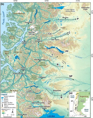
The Andean Cordillera dominates the landscape in the west (Figure 1), with local summit elevations of up to ∼2600 m a.s.l., before an eastward transition through the Patagonian foothills, which grade into the Argentine steppe. Ice originated from the Chilean highlands, advancing west towards the Pacific and east into present-day Argentina. During deglaciation, Atlantic-bound meltwater was stored in large proglacial lakes formed in overdeepened glacial troughs east of the ice divide (cf. Davies et al., 2020; García et al., 2019). Further ice recession then led to the opening of palaeolake drainage routes through the Andean Cordillera (cf. García et al., 2019). Today, ≥1482 glaciers remain in the region (Arendt et al., 2017); most of these are found adjacent to the Queulat ice cap (44.4° S, ∼2000 m a.s.l.), and Mt. Hudson volcano (45.9° S, ∼1900 m a.s.l.).

3. Previous mapping

Caldenius (1932) first mapped glacial landforms and glaciolacustrine sediments in the study area. Since this time, a number of early field surveys (e.g. Beltramone, 1991; Dal Molin, 1998; Lapido, 2000; Ploszkiewicz, 1987; Ramos, 1981) highlighted the largest and most extensive landforms, including moraine complexes or deposits, and proglacial outwash plains (Table 1 and Figure 2).

Figure 2. The location of published mapping between 44° and 46°S. Mapping type has been included: field or remotely sensed, as well as mapping extent. Where detailed maps or georeferenced locations were not available (Table 1), mapping extent has been estimated according to the data that has been described in each publication (legend: previous mapping). Areas that were field verified in this study have also been included (grey boxes). Modern ice extent from RGI v. 6.0, region 17 (Arendt et al., 2017). LGC/BA: Lago General Carrera-Buenos Aires.

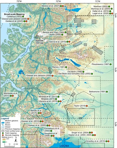
Table 1. Relevant glacial geomorphological landforms and glacier inventories presented in studies from Figure 2, described using the terminology presented in this paper.

Reference	Mapping Area Coverage	Mapping relevant to the new inventory
Caldenius (1932)^a	Broad-scale	Moraine complexes or deposits and glaciolacustrine sediments.
Ramos (1981)	Lago Plata-Fontana	Moraine complexes or deposits and proglacial outwash plains.
Ploszkiewicz (1987)	East of the Río Cisnes valley	Proglacial outwash plains.
Beltramone (1991)	Central Simpson/Paso Coyhaique	Moraine complexes or deposits, moraine ridges, and glaciolacustrine sediments.
Dal Molin (1998)	Lago Coyt/Río Ñirehuao, Simpson/Paso Coyhaique, and Balmaceda	Moraine complexes or deposits, glaciolacustrine sediments, and proglacial outwash plains.
Dal Molin and González Díaz (2002)	Lago Coyt/Río Ñirehuao, Simpson/Paso Coyhaique, and Balmaceda	Moraine ridges, proglacial outwash plains, and proglacial outwash terraces.
Escosteguy et al. (2003)	Eastern side of Lago Buenos Aires	Moraine complexes or deposits, glaciolacustrine sediments, and proglacial outwash plains.
Singer et al. (2004); Kaplan et al. (2004, 2005)	Eastern side of Lago Buenos Aires	Moraine complexes or deposits and glaciolacustrine sediments.
Glasser and Jansson (2005)	Lago Coyt/Río Ñirehuao, Balmaceda and Andean Cordillera	Moraine ridges, glacially scoured bedrock, glacial lineations, and meltwater channels.
Douglass et al. (2006)	Eastern side of Lago Buenos Aires	Moraine complexes or deposits, proglacial outwash plains, and glaciolacustrine sediments.
Glasser and Jansson (2008)	Broad-scale	Moraine ridges, trimlines, meltwater channels, proglacial outwash plains, glacial lineations, palaeolake shorelines, and cirques.
Glasser et al. (2009)	Western margins of Lago Buenos Aires, inside the Anean Cordillera	Moraine ridges, trimlines, glacially scoured bedrock, cirques, glacial lineations, meltwater channels, proglacial outwash plains.
Haller et al. (2010)	Lago Palena/General Vintter	Moraine complexes or deposits and moraine ridges.
Mardones et al. (2011)	Western edge of Simpson/Paso Coyahique, Balmaceda, and inside the Andean Cordillera	Cirques, moraine ridges, moraine complexes or deposits, and palaeolake shorelines.
Beraza & Vilas (1989) cited in: Rabassa et al. (2011)^a	Río Pico	Moraine complexes or deposits.
Martínez (2002) and Martínez et al. (2009) cited in: Martínez et al. (2011)^a	Lago Palena/General Vintter	Moraine complexes or deposits and moraine ridges.
Lapido (2000) cited in: Rabassa et al. (2011)^a	Río Pico	Moraine complexes or deposits and proglacial outwash terraces.
Davies and Glasser (2012)	Andean Cordillera	Moraine ridges, trimlines, and cirques.
Glasser et al. (2012)	Western edge of Lago Buenos Aires, inside the Andean Cordillera	Moraine ridges, trimlines, meltwater channels, proglacial outwash plains, palaeolake shorelines, glacial lineations, and cirques.
Miranda et al. (2013)^a	Simpson/Paso Coyahique and Balmaceda	Moraine complexes or deposits and moraine ridges.
Miranda (2015)^a	Simpson/Paso Coyahique and Balmaceda	Moraine ridges.
Smedley et al. (2016)	Eastern side of Lago Buenos Aires	Moraine ridges, palaeochannels, palaeolake shorelines, glaciolacustrine sediments, and proglacial outwash plains.
Bendle et al. (2017b)	Lago Buenos Aires	Moraine complexes or deposits, moraine ridges, trimlines, glacial lineations, glaciolacustrine sediments, perched deltas, palaeolake shorelines, proglacial outwash plains, catastrophic flood landforms, and meltwater channels.
García et al. (2019)	Río Cisnes	Moraine complexes or deposits, moraine ridges, palaeolake shorelines, perched deltas, and proglacial outwash plains.
Taylor (2019)	Eastern side of Balmaceda	Moraine complexes or deposits, moraine ridges, glacial lineations, meltwater channels, proglacial outwash plains, palaeolake shorelines, glaciolacustrine sediments, and perched deltas.
Vilanova et al. (2019)^a	Simpson/Paso Coyahique and Balmaceda	Moraine ridges.
Davies et al. (2020)	Broad-scale	Moraine ridges, trimlines, glacial lineations, meltwater channels, palaeolake shorelines, perched deltas, proglacial outwash plains, cols, and cirques.
Leger et al. (2020)	Lago Palena/General Vintter	Moraine complexes or deposits, moraine ridges, kettle holes, proglacial outwash plains, meltwater channels, catastrophic flood landforms, palaeolake shorelines, perched deltas, glaciolacustrine sediments, glacial lineations, glacially scoured bedrock, and cirques.
Moreno et al. (2021)	Northern tip of Lago Rosselot, inside the Andean Cordillera	Moraine complexes or deposits and moraine ridges.

^a Indicates studies where detailed maps have not been available, where the original publication was not accessible, or where landforms have been described, but precise mapping locations are unknown and cannot be fully reviewed.

In the Río Pico valley, five moraine complexes were mapped in association with an eastward-draining outlet glacier (Beraza & Vilas, 1989 and Lapido, 2000 In: Rabassa et al., 2011). Likewise, in the Río Cisnes valley, García et al. (2019) mapped five main moraine complexes (Named: CIS 1, 2, 3, 4, and 5) and identified the limits of a proglacial palaeolake. Distinct palaeolake shorelines at 950-920 m a.s.l. and 860-850 m a.s.l. can be traced from the upper-to-middle Río Cisnes valley (Davies et al., 2020; García et al., 2019). A col located at ∼920 m a.s.l. drained the palaeolake towards the Atlantic Ocean at this level (Davies et al., 2020), whilst the prominent Winchester Delta (Figure 3), south of the modern Río Cisnes, clearly marks the ∼860-850 m a.s.l. lake level (García et al., 2019).

Figure 3. Broad geomorphological context of mapped valleys, including key moraine complexes. It is likely that the stratigraphically oldest moraine complexes span multiple glacial advances. Moraine complexes were mostly identified from remote mapping and should be field verified. Outlet glaciers: P: Río Pico, Ca: Río Caceres, C: Río Cisnes, PF: Lago Plata-Fontana, T: El Toqui, Ñ: Lago Coyt/Río Ñirehuao, SP: Simpson/Paso Coyhaique, and B: Balmaceda. Location and extent of maps presented in Figures 4–6 have also been included (black boxes) and photos of glaciolacustrine sediments (red dots). Modern ice extent from RGI v. 6.0, region 17 (Arendt et al., 2017).

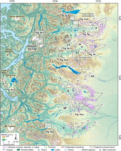
Figure 4. Ice-marginal landforms within the main outlet valleys and the Andean Cordillera. Raw satellite images (left) and mapped geomorphology (right). (a) Satellite image of central-northern sector of the Río Pico valley, including the location of (g). (b) Mapped landforms, including the PIC 6 moraine and an associated proglacial outwash plain. (c) Satellite image of a morainal bank, which is the lateral margin of the PIC 6 moraine, and a small isolated palaeolake basin in the northern Río Pico valley. (d) Mapped landforms surrounding the PIC 6 morainal bank, which is adjacent to ice-contact fans, and multiple, stepped, palaeolake shorelines. (e) Satellite image of the area southeast of the Queulat ice cap. (f) Mapped moraines and trimlines associated with the stratigraphically youngest glacier advances in the Andean Cordillera. (g) Ice-proximal view of the PIC 6 moraine in the field overlooking older moraines and terminating into a proglacial outwash plain. Satellite images are from ESRI™ DigitalGlobe World Imagery via ArcGIS Pro. Figure panel locations are shown in Figure 3.

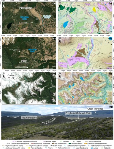
Figure 5. Subglacial and glaciolacustrine landforms and sediments. (a) Satellite image of glacial lineations in the Simpson/Paso Coyhaique valley. (b) Mapped glacial lineations in the Simpson/Paso Coyhaique valley, dissected by proglacial outwash plains. Glacial lineations are aligned in a west-east and southwest-northeast direction, and adjacent to moraine complexes or deposits. (c) Satellite image of recently deglaciated ice cap south of Volcán Macá. (d) Flutes mapped within the Andean Cordillera which demonstrate multiple, diverging, local ice-flow directions. (e) Satellite image of the CIS 4 moraine, Río Cisnes valley. (f) Short-lived, narrow, palaeolake shorelines embedded on the CIS 4 moraine. (g) Laminated glaciolacustrine sediments located in the centre of the Río Pico palaeolake basin. (h) Glaciolacustrine sediments dissected by a tephra layer (cf. Stern et al., 2015) in the Río Cisnes valley.

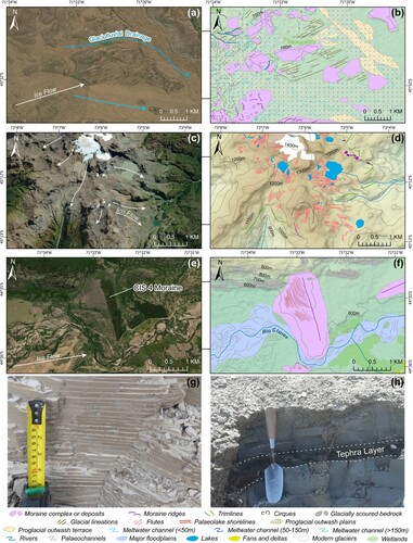
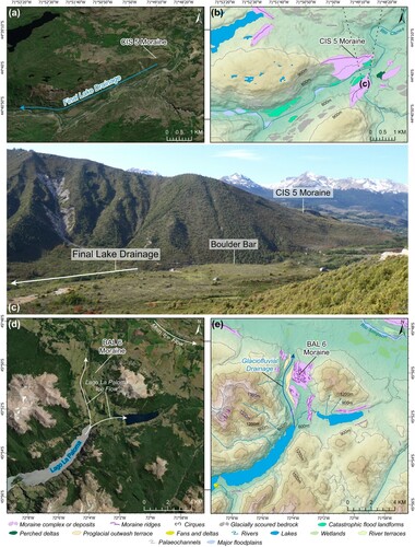
Figure 6. Examples of glaciofluvial landforms in the study area. (a) Location of catastrophic flood landforms and direction of final palaeolake drainage in the Río Cisnes valley. (b) Mapped catastrophic flood landforms along the banks of the modern Río Cisnes, adjacent to the CIS 5 moraine. Includes the location of (c). (c) Catastrophic flood landform in the foreground, adjacent to the CIS 5 moraine. (d) Location and ice-flow direction at Lago La Paloma, the site of a tributary glacier of the main Balmaceda valley. (e) Mapping of the La Paloma glacier, including moraine ridges and proglacial outwash terraces. Proglacial outwash terraces indicate that glaciofluvial drainage from the La Paloma glacier was directed towards the main Balmaceda valley.

Beltramone (1991) identified multiple moraine complexes or deposits and moraines associated with the Simpson/Paso Coyhaique glacier (Figure 2). Dal Molin (1998) and Dal Molin and González Díaz (2002) further mapped broad moraine complexes and proglacial outwash plains from the Lago Coyt/Río Ñirehuao to Balmaceda valleys, east of the international boundary. Glasser and Jansson (2005) then used satellite remote sensing data to map in greater detail and presented the first indication of fast ice-flow in the region, evidenced by glacial lineations. Subsequently, Taylor (2019) provided thorough mapping of the Balmaceda outlet glacier (Table 1). This included the identification of previously unmapped moraine complexes and ridges associated with several glacial advances, proglacial outwash plains, and multiple palaeolake levels.

Within the Andean Cordillera, Mardones et al. (2011) mapped moraines deposited in tributary valleys of the main Balmaceda outlet glacier (Figure 2 and Table 1). Davies and Glasser (2012) then identified late-Holocene moraines and trimlines, allowing an assessment of recent ice extent. Multiple studies have now provided mapping within the Andean Cordillera (Glasser & Jansson, 2005, 2008; Mardones et al., 2011; Moreno et al., 2021), but at variable spatial scales.

The PATICE database compiled and generated new mapping (Table 1) for the entire PIS (Davies et al., 2020). In the area located between 44° and 46° S, detailed mapping has been limited to the Río Cisnes valley (e.g. García et al., 2019), and a regional, high-resolution, inventory is needed to assess palaeoglaciological processes.

4. Methods

Mapping of the eastern outlet glaciers was completed at 1:10,000–1:40,000 spatial scales, and a 1:1000–1:10,000 scale was used inside the Andean Cordillera. Landform identifications were undertaken according to descriptions outlined by Bendle et al. (2017b, pp. 660–661), Martin et al. (2019, pp. 114–115), and Leger et al. (2020, pp. 654–656), following protocols outlined in Chandler et al. (2018). Identification criteria were then modified for the study area (Table 2). Where possible, published landforms were re-mapped and incorporated into the new inventory (Table 1). River and proglacial outwash plain shapefiles were adapted from the PATICE database (Davies et al., 2020), and modern glaciers were extracted from the Randolph Glacier Inventory (RGI v. 6.0, region 17; Arendt et al., 2017).

Table 2 . Rationale, uncertainties, and identification criteria for ice-marginal, subglacial, glaciolacustrine, glaciofluvial, and non-glacial landforms mapped between 44 – 46°S. Total mapped landform numbers and/or areas are provided where applicable. Landform occurrence (✘) within the study region: P: Río Pico outlet glacier, Ca: Río Caceres outlet glacier, C: Río Cisnes outlet glacier, PF: Lago Plata-Fontana outlet glacier, T: El Toqui outlet glacier Ñ: Lago Coyt/Río Ñirehuao outlet glacier, SP: Simpson/Paso Coyhaique outlet glacier, B: Balmaceda outlet glacier, and A: landforms mapped within the Andean Cordillera. Identification criteria were modelled after Bendle et al. (2017b), Martin et al. (2019), and Leger et al. (2020): criteria were then modified and updated for the study area.

Landform	Rationale	Uncertainties	Identification criteria	Number of observations	Area (km^2)	Landform occurrence
						P	Ca	C	PF	T	Ñ	SP	B	A
Ice-marginal landforms
Moraine complexes or deposits	Indicates lateral/terminal extent of a glacier. Representative of prolonged glacier stillstands or (re-)advances.	It can be difficult to differentiate between consecutive glacial advances from satellite imagery alone. May be confused with landslides or slumps when plastered onto the valley sides.	In satellite imagery, elongate ridges or crests found in close proximity. Older deposits may possess gently undulating mounds, with no distinct moraine ridges and are sometimes heavily eroded. Can often be traced for long distances and may be found adjacent to proglacial outwash plains.	–	1487	✘	✘	✘	✘	✘	✘	✘	✘	–
Moraine ridges	Indicates glacier lateral or terminal extent at the time of deposition. Moraine size may inform on the relative longevity of the ice-margin position.	Moraines lacking sharp or significant relief may be difficult to detect in satellite imagery. Small moraine ridges associated with younger glacial advances in the Andean Cordillera usually require mapping at a high spatial resolution (≤1:10,000).	In satellite imagery, elongate ridges or crests with positive relief. Often steeply sloping or gently sloping on one side. May be flat-topped in some cases. Likely to possess dark-light shading from relief. In the field, likely to also be topped with boulders and cobbles.	11307	–	✘	✘	✘	✘	✘	✘	✘	✘	✘
Morainal banks	Indicative of a glacier that was calving into an ice-contact lake.	In satellite imagery, may be easily overlooked and confused with other moraine ridges when palaeolake evidence is not apparent.	In satellite imagery, a rounded wedge of sediment that possesses a steep ice-distal slope, with a gently tapering ice-proximal slope. Found in close proximity to palaeolake shorelines or ice-contact fans.	1	5.9	✘	–	–	–	–	–	–	–	–
Trimlines	Indicative of recent ice extent (ice-marginal trimlines) or thickness (lateral trimlines).	When mapping remotely, trimlines may be difficult to distinguish from small, low-relief, latero-frontal moraines within the Andean Cordillera. Requires a high spatial resolution to map remotely (≤ 1:10,000).	Trimlines are found within the Andean Cordillera. In satellite imagery, trimlines possess an ovate morphology, or run horizontally with the valley walls, pointing down-valley. A distinct transition between glacially scoured bedrock, sediment, or low-lying vegetation and the developed treeline is apparent.	505	–	–	–	–	–	–	–	–	–	✘
Subglacial landforms
Cirques	Informs on origin of local ice-sources.	Identification may be hindered by presence of snow cover or vegetation in satellite imagery.	In satellite imagery, arcuate hollows with steep headwalls, found on mountaintops are interpreted as cirques. Cirques are mostly found inside the Andean Cordillera. May be located above small moraines or trimlines. May contain a lake.	1942	–	✘	✘	✘	✘	✘	✘	✘	✘	✘
Crag-and-Tails	Oriented parallel to the direction of local ice-flow.	Can be difficult to distinguish from bedrock outcrops or glacial lineations when using satellite imagery alone. Field verification is required to confirm landform interpretation.	In satellite imagery, crag-and-tails are oriented in the direction of local ice-flow. Ovate mounds which elongate and become pointed on their down-ice slope. Bedrock may protrude from their up-ice (stoss) end. In the field, a resistant bedrock core can be found on their stoss end. A gently tapering lee slope composed of glacial sediments is elongated in the direction of ice-flow. Usually plastered with faceted boulders and cobbles.	20	–	–	–	✘	–	–	–	–	–	–
Glacially scoured bedrock	May indicate former ice-flow direction, wet-based ice, or areas where ice was thick.	In satellite imagery, bedrock is often plastered with surficial sediments or interspersed with vegetation which may hinder identification.	In remote mapping, extensive areas of bedrock within former ice limits which appear smoothed. May appear streamlined in the direction of ice-flow. In the field, may additionally be found overlain with perched boulders or interspersed with subglacial diamict.	4725	195	✘	✘	✘	✘	✘	✘	✘	✘	–
Glacial lineations	Will signal the direction(s) of former ice-flow. May be indicative of fast-flowing or streaming ice.	May not be identifiable in highly vegetated areas. Could be confused with crag-and-tails or moraine ridges.	In satellite imagery, elongate ridges with sharp-to-gently tapering sides oriented in the direction of ice-flow. ≤2.5 km in length and ≤0.1 km in width, regionally. Often found aligned with moraine complexes or deposits.	257	–	✘	–	✘	–	–	✘	✘	✘	–
Flutes	Signal the direction(s) of local ice-flow. Indicates areas which were recently glacierised.	Flutes are only preserved near active or recently active glaciers. Requires high-resolution (≤ 1:10,000) mapping from satellite imagery to identify remotely.	Mapped remotely and found within the Andean Cordillera. Found down-slope of active glaciers or recently deglacierised areas. Elongate, thin, ridges of glacigenic sediment, oriented in the direction of ice-flow. Found in swarms.	2521	–	–	–	–	–	–	–	–	–	✘
Glaciolacustrine l andforms
Palaeolake shorelines	Indicative of palaeolake surface elevation, lake level longevity, and the lateral extent of the palaeolake.	Difficult to distinguish when not continuous in satellite images. May be confused with low-relief moraines. In the field, narrow shorelines with closely spaced steps are difficult to map individually.	In satellite imagery 1) elongate, flat-topped ridges which may be traced for significant distances. May possess a steep lake-marginal slope or be found in association with perched deltas or ice-contact fans. 2) Short-lived, discrete, palaeolake shorelines are found in sets, and possess narrow terracing and closely spaced steps. Both shorelines are identifiable by dark-light shading in satallite imagery. In the field, palaeolake shorelines may possess a flat or gently-undulating surface.	2121	–	✘	✘	✘	✘	–	✘	✘	✘	–
Perched deltas	Can be used to indicate a proglacial palaeolake level. May help to infer the lateral extent of a palaeolake.	May be misinterpreted as an alluvial fan in satellite imagery, particularly when the elevation change between the delta-top area and surrounding landscape is not sharp.	In satellite imagery, perched deltas possess a flat top, and sharp or gently sloping lake-marginal slope. Usually fan-shaped in plan view. Will be found pointing towards a lake or palaeolake basin, and may be associated with, or raised above, palaeolake shorelines. May preserve palaeochannels, gullies, or contain modern rivers.	91	50	✘	✘	✘	✘	✘	✘	✘	✘	–
Ice-contact fans	Indicative of ice-contact lake presence and surface elevation at the time of moraine deposition. May provide an approximate ice extent.	In satellite imagery, may be mistaken for proglacial outwash plains or perched deltas where topography is subdued or palaeolake/moraine evidence is not clear.	In satellite imagery, ice-contact fans possess a similar morphology to perched deltas. Additionally found on the ice-distal side of moraines and perched above the palaeolake basin. May preserve meltwater channels on their surface.	16	23	✘	✘	–	✘	–	–	–	✘	–
Glaciolacustrine sediments	Indicates the presence of a palaeolake. May provide further information on processes of glaciolacustrine sediment deposition.	Requires field or laboratory verification to assess model of glaciolacustrine sediment deposition. May be difficult to identify in heavily vegetated areas.	In the field, possess a laminated or homogenous matrix. Likely to be exposed where rivers or runoff have incised older glaciolacustrine sediments. At the macro-scale, laminated glaciolacustrine sediments contain moderate-to-well-sorted laminae comprised of clays, silts, and sands. In satellite imagery, usually appear beige or white in colour, and are located near a modern lake or within a palaeolake basin.	–	–	✘	–	✘	–	–	–	✘	✘	–
Palaeolake spillways (cols)	Indicative of palaeolake drainage outlet and direction of glaciofluvial drainage.	In satellite imagery, may be difficult to discern when landscape has been dissected by younger glaciofluvial drainage routes. May be mistaken for gullies.	By generating contours in GIS, and corresponding these with known palaeolake levels, drainage outlets may be identified at these levels. Will usually be marked by a large palaeochannel directed towards an area of lower relief.	5	–	✘	–	✘	–	–	✘	–	✘	–
Glaciofluvial landforms
Catastrophic flood landforms	Provides evidence for the occurrence of catastrophic floods. May also provide insight into the direction of flood drainage.	May be confused with river terraces in satellite imagery. Field verification is necessary for identification.	In satellite imagery, flat-topped landforms with steep scarp slopes which possess a similar morphology to river terraces. In the field, identifiable by presence of large boulders (≤3 m in height) which are located within and on top of a boulder bar.	12	–	–	–	✘	–	–	–	–	–	–
Proglacial outwash plains Adapted from Davies et al. (2020) PATICE shapefiles.	Indicative of meltwater drainage direction. May inform on ice-margin extent.	Older proglacial outwash plains may be difficult to distinguish where glaciofluvial drainage routes meet.	In satellite imagery, usually possess extensive networks of braided meltwater channels. Usually found on the ice-distal side of moraines and moraine complexes or deposits.	–	18144	✘	✘	✘	✘	✘	✘	✘	✘	✘
Proglacial outwash terraces	May indicate the relative longevity of glaciofluvial drainage routes.	May be confused with river terraces near modern drainage routes. Difficult to delineate the limits of multiple terraces without field verification.	In satellite imagery, found within areas of proglacial outwash plains. Terraces are raised above surrounding proglacial outwash plains, and possess a steep scarp slope identifiable through light-dark shading.	352	93	✘	✘	✘	✘	–	✘	✘	✘	–
Meltwater channels Classified as: <50 m width 50–150 m width >150 m width	Indicates the direction(s) of glaciofluvial drainage. Preservation may reveal the relative age of drainage routes. May indicate the approximate and relative position of the ice-margin.	May be mistaken for palaeochannels (e.g. proglacial meltwater channels) or gullying in satellite imagery. May be occupied by modern drainage. In the field, proglacial meltwater channels within proglacial outwash plains are difficult to discern.	When mapping remotely, proglacial meltwater channels appear sinuous to braided, possess a dark-light shading, and are found in large numbers within proglacial outwash plains. Ice marginal and subglacial meltwater channels appear sinuous, and cross-cut moraines and moraine complexes or deposits. May be occupied by modern drainage or wetlands.	31648	–	✘	✘	✘	✘	–	✘	✘	✘	–
Kettle holes	Indicative of an area of deposition. May suggest a stagnant ice margin	When mapped remotely, kettle holes are easily confused with small lakes.	In satellite imagery, kettle holes possess an ovate or sub-rounded planform shape. Hollows may contain small lakes, and are found within proglacial outwash plains or moraine complexes or deposits.	1572	–	✘	–	✘	–	✘	✘	✘	✘	–
Non-glacial landforms
Fans or deltas	When present, may indicate reworking of underlying sediments.	Fans may be confused with perched deltas in satellite imagery, particularly when palaeolake shoreline evidence is not apparent.	Both in satellite imagery and in the field: fan shaped in plan view, may be gently sloping towards the main river channel or lake. May contain active or palaeochannels on their surface.	1506	263	✘	✘	✘	✘	✘	✘	✘	✘	✘
Rivers Adapted from Davies et al. (2020) PATICE shapefiles.	Indicates the origin and direction of modern drainage routes.	Smaller tributary rivers may be difficult to map in heavily vegetated areas.	Straight, sinuous, or braided channels, which can be traced for a significant distance. Usually contain contemporary drainage.	–	–	✘	✘	✘	✘	✘	✘	✘	✘	✘
Palaeochannels	Indicates the presence and extent of past drainage routes.	May be mistaken for proglacial meltwater channels when modern rivers are occupying proglacial outwash plains.	Will usually be found next to active river channels, may retain water if recently abandoned (e.g. oxbow lakes). Sinuous-to-braided morphology.	9732	–	✘	✘	✘	✘	–	✘	✘	✘	✘
River terraces	Indicates the extent of the former floodplain and the possible re-working of sediments.	May be misinterpreted as a proglacial outwash terrace where modern fluvial drainage is cutting through proglacial outwash plains.	Flat-topped sediment accumulations which possess a steep scarp slope. Found adjacent to modern rivers, floodplains, or palaeochannels.	493	36	–	–	–	–	–	–	–	–	✘
Major floodplains	Determines lateral extent of modern fluvial activity.	Difficulties in distinguishing between floodplains and wetlands when these landforms coincide.	Will often be covered with low-lying vegetation. May appear waterlogged in satellite imagery. Found adjacent to rivers.	–	311	✘	✘	✘	✘	✘	✘	✘	✘	–
Lakes	May indicate the presence of palaeolake shorelines or perched deltas.	In satellite imagery, small water bodies may be mistaken for kettle holes in the main outlet valleys.	Water bodies of varying sizes which may be frozen.	3299	2793	✘	✘	✘	✘	✘	✘	✘	✘	✘
Landslides or slumps	Indicates areas where underlying landforms and sediments have been re-mobilised.	When mapping remotely, landslides or slumps may be mistaken for lateral moraines, particularly when the source of the slope failure is not apparent.	In satellite imagery, slumped material containing irregular or undulating ridges. Usually found below a rounded hollow or scar which may be identified as the source of the slope failure.	40	123	–	–	–	–	–	✘	✘	✘	✘
Wetlands	May indicate areas of recent fluvial activity or re-working.	May be mistaken for floodplains in satellite imagery when near modern rivers.	In satellite imagery, usually appear green and saturated in comparison to the surrounding landscape. Covered with low lying vegetation. Found adjacent to rivers or lakes.	–	1550	✘	✘	✘	✘	✘	✘	✘	✘	–
			Total	72165	25073.9

Mapping was completed with ArcGIS Pro using the Southern Hemisphere WGS-1984-UTM Zone 18S Projected Coordinate System. A ∼50,000 km² area was mapped using an ASTER (v.3) 30 m resolution Digital Elevation Model (ASTER DEM). Composite ESRI™ DigitalGlobe World Imagery (1–2 m resolution) and Sentinel-2 (10 m resolution) imagery were used to identify landforms. Hillshade and Slope Digital Terrain Models were generated using the Spatial Analyst function and overlain onto the ASTER DEM to highlight topographic relief and elevation (Otto & Smith, 2013). Field surveys validated geomorphological interpretations at multiple locations (Figure 2).

5. Mapped landforms

Mapping was classified into ice-marginal, subglacial, glaciolacustrine, glaciofluvial, and non-glacial landform categories (Table 2). Within these groups, a total of 27 landform types were digitised, which resulted in a database of >70,000 mapped features. We describe landforms mapped in the eight outlet valleys and the Andean Cordillera.

5.1. Ice-marginal landforms

5.1.1. Moraine complexes or deposits

Arcuate moraine complexes were deposited by the main outlet glaciers, and extend over tens of kms across the mouths of the individual valleys. Moraine complexes or deposits were mapped in multiple previous publications and have been re-mapped in greater detail. Herein, moraine complexes have been named to follow a standard nomenclature (Figure 3).

Moraines can be grouped into sets (moraine complexes) using morphostratigraphy to determine the relative ice-margin age (cf. Lukas, 2006) prior to developing geochronological datasets (Lüthgens & Böse, 2012). Moraine complexes or deposits were defined from satellite imagery based on geographic position, as well as moraine morphology and proximity. Where available, proglacial outwash plains were also used to identify the lateral and terminal extent of moraine complexes. However, the easternmost moraine complexes commonly lack distinct moraine ridges and are instead comprised of mounds or flat-topped and irregular terrain. In particular, the limits of older or proximal moraine complexes or deposits (e.g. Figure 3: SPC 1) can become difficult to define and should be field verified.

5.1.2. Moraine ridges

Moraine ridges mark the extent of past glacial advances, readvances, or stillstands (e.g. Davies et al., 2020; Glasser & Jansson, 2008) and define the geometry of the glacier terminus (Ely et al., 2021). Moraine ridges were mapped in all outlet valleys and within the Andean Cordillera.

Strings of latero-frontal moraines cap the eastern margins of the former outlet glaciers. Moraine morphology varies between straight, arcuate, or meandering ridges (Figure 4(a,b)) or mounds, ranging from <0.01 km to ∼50 km in length (Figure 3). In the field, the moraine crest/apex usually possesses an undulating morphology (Figure 4(f)) and are commonly overlain with sub-rounded, faceted boulders. The highest relief (ca 250 m) and most distinctive of these possess a sharp apex, steep ice-distal slope, and crosscut the Río Cisnes valley (CIS 3, 4 & 5; García et al., 2019). The longest moraine in the region is found in the Río Pico valley, a laterally continuous moraine (∼50 km in length), with a sinuous morphology (Figure 3 and Figure 4(a,b)).

Within the Andean Cordillera, stratigraphically younger moraines are usually low-relief (<10 m), continuous ridges that possess an arcuate form and point down-slope of empty and occupied mountaintop cirques (e.g. Figure 3). Straight or winding, discontinuous ridges with close spacing are found nested up-slope of larger latero-frontal moraines. The best preserved of these are found surrounding the Mt. Hudson volcano.

5.1.3. Morainal banks

A rounded wedge of sediment, possessing a steep ice-distal face, and gently tapering ice-proximal slope (44°03′32.8″ S, 71°34′22.9″ W) has been mapped adjacent to palaeolake shorelines and ice-contact fans in the northern Río Pico valley. This landform has been interpreted as a morainal bank (cf. Fitzsimons & Howarth, 2018; Rovey & Borucki, 1995), indicating a glaciolacustrine terminus with subaqueous deposition (cf. Davies et al., 2018; Martin et al., 2019). The morainal bank marks the northern lateral edge of the PIC 6 moraine (Figure 4(c,d)), aligned in a south-north direction, ∼5 km in length, and terminating into a small (∼12 km²), isolated, palaeolake basin (44°01′56.7″ S, 71°32′57.0″ W).

5.1.4. Trimlines

Trimlines were mapped within the Andean Cordillera (e.g. Figure 4(e,f)), and are concentrated around the remaining ice caps (e.g. Figure 3). Trimlines are found in two forms: the first is lobate landforms, which possess a sharp or gradational break between glacially scoured bedrock, sediment, or shrubs to the developed treeline, and point down-valley from active glaciers or abandoned cirques. The second possesses a sharp transition between underlying sediment/bedrock to low-lying shrubs and run parallel with the valley sides. According to criteria outlined by Rotes and Clark (2020), these are classified as glacial trimlines based on a clear contrast between surface age (e.g. developed vegetation, glacially scoured bedrock), proximity to moraines, or position down-slope of glaciers.

5.2. Subglacial landforms

5.2.1. Cirques

Landforms identified on mountain tops in the Andean Cordillera and marked by arcuate headwalls which taper into sub-rounded erosional hollows are mapped as cirques (Figure 4(e,f)). Many cirques in Patagonia still contain glaciers (e.g. Araos et al., 2018; Martin et al., 2019), though here we map abundant deglacierised cirques. Cirques can be identified in the surrounding landscape based on their position up-slope of ice-marginal (e.g. latero-frontal moraines) and subglacial (e.g. flutes, glacially scoured bedrock) landforms. The cirque bed will often appear overdeepened from subglacial erosion (Hooke, 1991), and sometimes contains a lake.

5.2.2. Crag-and-Tails

Crag-and-tails can be differentiated from other subglacial landforms by a resistant bedrock core on their up-ice (stoss) end, with a gently tapering lee slope composed of softer glacial sediments (Benn & Evans, 2014; Stroeven et al., 2013). Elongate ridges (individually ≤2 km in length, ≤0.4 km in width), only mapped in the Río Cisnes valley, are interpreted as crag-and-tails, aligned southwest-northeast and streamlined in the direction of local ice-flow.

5.2.3. Glacially scoured bedrock

Glacially scoured bedrock is distinguishable from the surrounding landscape by a smoothed bedrock surface often interspersed with vegetation, till, or found overlain with perched boulders. These glacial erosional landforms may indicate points of greater ice thickness, where basal ice has reached its pressure-melting point (Glasser & Bennett, 2004; Shaw, 1994). Similarly to the more northerly Río Corcovado, Río Huemul, and Lago Palena-General Vintter glaciers (Leger et al., 2020, ∼43° S), the Río Pico valley possesses extensive areas of glacially scoured bedrock (∼84 km²), and displays a broad-scale west–east streamlining in the direction of local ice-flow.

5.2.4. Glacial lineations

Glacial lineations are defined by an ovate or linear, elongate morphology, valley-floor position, and orientation in the direction of ice-flow. These landforms can be utilised as flow lines and may indicate areas of thick or warm-based ice that scoured and deposited sediment into linear ridges (Glasser & Jansson, 2005; Stroeven et al., 2013). Regionally, the most well-defined, elongate (≤2.5 km in length) and narrow (≤0.1 km in width) ridges occur in the Simpson/Paso Coyhaique valley (e.g. Figure 5(a,b)), aligned west–east and southwest–northeast reflecting local ice-flow directions.

5.2.5. Flutes

Narrow, elongate, and streamlined ridges (≤1.5 km in length) are a product of subglacial deformation (cf. Van der Meer, 1997), and were mapped as sedimentary flutes. Flutes are only preserved within recently deglacierised areas, and are useful in determining the direction(s) of local ice-flow (Gordon et al., 1992). We mapped 2521 flutes on mountaintops within the Andean Cordillera. The best example of these can be found south of Volcán Macá (Figure 5(c,d)), up-valley of glacial trimlines, and demonstrating multiple, diverging, ice-flow paths.

5.3. Glaciolacustrine landforms

5.3.1. Palaeolake shorelines

In Patagonia, during glacial maxima, erosion of sediment/bedrock beneath outlet glaciers formed glacial overdeepenings (cf. Cook & Swift, 2012), which were sometimes exposed subaerially during deglaciation. These overdeepenings commonly developed into proglacial lakes during deglaciation (e.g. García et al., 2019; Leger et al., 2020). In the study area, most of these lakes have now drained, leaving well-preserved palaeolake shorelines to mark their former extent (Davies et al., 2020; García et al., 2019).

We mapped palaeolake shorelines in two common forms. The first is continuous, flat-topped terraces calved into valley sides, moraines, or associated with perched deltas. These shorelines represent the most long-lived lake levels in the region. The largest and most distinctive of these shorelines are found in the Río Cisnes valley at 950–920 m a.s.l., and 860–850 m a.s.l. (Davies et al., 2020; García et al., 2019), and the Río Pico valley at ∼870 m a.s.l.

The second type is sets of multiple, discontinuous, shorelines found on moraines or eroded into valley-side deposits (Figure 5(e,f)). These are more difficult to discern in the field due to narrow terracing and closely spaced steps, and represent a punctuated lake level lowering through time (e.g. Bell, 2008; Thorndycraft et al., 2019a). These sets are found in the Río Pico (1010–910 m a.s.l.), Río Cisnes (790–650 m a.s.l.), Lago Coyt/Río Ñirehuao (730–600 m a.s.l.) and Balmaceda (∼600–610 m a.s.l.) valleys.

5.3.2. Perched deltas

Perched deltas formed when rivers met proglacial lakes and remained raised above the (palaeo-)lake basin as lake levels fell (e.g. Dulfer & Margold, 2021; Stroeven et al., 2016). Perched deltas are flat-topped or possess a gentle slope oriented towards, but elevated above, a palaeolake basin. Mapping the distribution and elevation of perched deltas, and comparing them with palaeolake shorelines, informs on the extent of former palaeolake levels (cf. Bell, 2008; Glasser et al., 2016; Turner et al., 2005). We mapped 91 perched deltas in the study area, the largest of these is the Winchester Delta (44°36′30.9″ S, 71°27′08.4″ W) in the Río Cisnes valley (García et al., 2019), marking a local palaeolake level of 860–850 m a.s.l. Large deltas are also found in the Río Pico valley (44°04′54.3″ S, 71°35′34.1″ W; 44°05′12.8″ S, 71°33′07.0″ W), associated with a ∼850 m a.s.l. delta-top area.

5.3.3. Ice-contact fans

Ice-contact fans morphologically resemble perched deltas but can be distinguished based on their proximity to moraines. These landforms are composed of a build-up of glaciofluvial outwash on the ice-distal side of moraines during a prolonged period of glacier stability (Dowdeswell et al., 2015), and indicate the former ice-contact lake level at the time of moraine formation. The largest ice-contact fan (∼15 km²) is found adjacent to the southern lateral margin of the PIC 6 moraine (44°24′48.4″ S 71°33′38.1″ W), gently sloping into the Río Caceres palaeolake basin, and marking a ∼900 m a.s.l. lake level.

5.3.4. Glaciolacustrine sediments

Caldenius (1932) first described glaciolacustrine sediments in the study region, but precise locations were previously unknown. Fine grained, well-sorted, and laminated glaciolacustrine sediments have accumulated in association with proglacial palaeolake formation during deglaciation (Figure 5(g,h)). At the macro-scale, these deposits resemble varved sediments studied at Lago Buenos Aires (Bendle et al., 2017a). Laminated glaciolacustrine sediments were field verified in the Río Pico, Río Cisnes, Simpson/Paso Coyhaique, and Balmaceda valleys.

5.3.5. Palaeolake spillways (cols)

We updated previous mapping of palaeolake spillways (cols) identified in the Río Cisnes, Lago Coyt/Río Ñirehuao, and Balmaceda valleys (Davies et al., 2020; García et al., 2019), which are important for studying the switch between Atlantic-bound and Pacific-bound drainage routes during deglaciation (Thorndycraft et al., 2019a; 2019b). We mapped two additional cols in the Río Pico valley at ∼810 m a.s.l. and ∼770 m a.s.l., by analysing contour elevations of known palaeolake shorelines in ArcMap. These data suggest that the Pico palaeolake drained east, towards the Atlantic, until the palaeolake level dropped below ∼770 m a.s.l.

5.4. Glaciofluvial landforms

5.4.1. Catastrophic flood landforms

We identified boulder bars in the middle Río Cisnes valley (∼470–560 m a.s.l.), above the banks of the modern Río Cisnes, and in association with the CIS 5 moraine (Figure 6(a–b)). The boulder bars are characterised by steep scarp slopes with a flat-topped surface, interspersed with sub-rounded boulders (≤3 m in height) and cobbles. In the field, we interpreted one boulder bar (44°40′08.0″ S, 71°49′06.6″ W, 545 m a.s.l.) as an expansion bar with a fossa channel located on the southern edge of the deposit (Figure 6(c)). These landforms are similar to those identified by Benito and Thorndycraft (2020) further south in the Baker valley, which were interpreted as forming as the result of catastrophic floods (>10⁵ m³/s) during palaeolake drainage.

5.4.2. Proglacial outwash plains

Proglacial outwash plains are characterised by broad, flat-topped expanses of glaciofluvial sediment, forming on the ice-distal side of moraines, or found nested between moraine complexes (e.g. Bendle et al., 2017b; Darvill et al., 2014). Similarly to moraine complexes, proglacial outwash plains may provide approximate ice-marginal positions but additionally indicate the direction(s) of glaciofluvial drainage. Mountainous areas to the east of the main outlet glaciers constrained the area of former glaciofluvial activity; beyond this, the landscape transitioned into the Argentine steppe, where proglacial outwash plains formed continental drainage networks (e.g. Clapperton, 1993).

5.4.3. Proglacial outwash terraces

Raised, flat-topped terraces of glaciofluvial sediment, located within the margins of proglacial outwash plains, are interpreted to form as a result of isostatic uplift (Maizels, 2002) or (glacio-)fluvial incision (Eilertsen et al., 2015). Stratigraphically younger terraces usually display well-preserved meltwater channels, whilst the surfaces of outwash terraces associated with the most extensive glacial advances appear homogenous. Based on geographic position, some of the stratigraphically youngest outwash terraces, oriented in a southwest–northeast direction, are found in a tributary valley of the Balmaceda glacier (Figure 6(d,e)).

5.4.4. Meltwater channels

Meltwater channels were mapped in the main outlet valleys, and in two main forms. The first are proglacial meltwater channels, which form extensive networks and are found on the ice-distal side of moraines, preserved on proglacial outwash plains (e.g. Bendle et al., 2017b; Leger et al., 2020). These are generally sinuous, discontinuous, channels with narrow spacing. The second are ice-marginal and subglacial meltwater channels that dissect moraine ridges (e.g. Figure 4(a,b)) or the valley floor. These channels are sinuous, vary in width from less than 50 m to over 150 m, and can only be traced for short distances. Where moraine complexes or ridges are heavily dissected, ice-marginal meltwater channels provide additional evidence for ice extent (Greenwood et al., 2007).

5.4.5. Kettle holes

Kettle holes were mapped inside proglacial outwash plains or nested within/between moraine complexes. Kettle holes are enclosed depressions with an ovate or sub-rounded planform shape and can be dry or contain small lakes. These landforms indicate regions where dead ice has been buried, melted, and left a residual pit (Evans & Orton, 2015). The largest kettle holes (∼2 km²) are located between the ÑIR 1 and ÑIR 2 moraine complexes, in the Lago Coyt/Río Ñirehuao valley.

5.5. Non-glacial landforms

Some non-glacial features were mapped in addition to glacial geomorphology. Holocene rivers, fans and deltas, palaeochannels, wetlands, and major floodplains determine the direction of modern or recent drainage routes and point to areas of possible post-depositional re-working. River terraces provide an indication of the relative age of drainage routes, and therefore the timing of continental drainage re-organisation. Mapping residual lakes can also be useful, particularly in determining the structure of palaeolake evolution in the main valleys.

Landslides or slumps were common following deglaciation, and particularly in the southern region (below 45.5° S) of the study area (cf. Pánek et al., 2021). Mapping landslides or slumps is important, as gravitational instabilities can be mistaken for moraines (e.g. Soteres et al., 2020). In particular, younger landslides or slumps appear to have overlaid segments of the Simpson/Paso Coyhaique and Balmaceda lateral moraine complexes.

6. Concluding points

We present a glacial geomorphological map covering a ∼50,000 km² area of west-central Patagonia (44–46° S), building on existing mapping in the region (Table 1). The map provides a detailed, georeferenced, inventory of glacial landforms mapped within eight outlet valleys and the Andean Cordillera. The inventory contains >70,000 features and 27 landform groups which were classified as ice-marginal, subglacial, glaciolacustrine, glaciofluvial, or non-glacial landforms. Our mapping reveals: (1) Multiple, previously unmapped, moraine complexes or deposits and ridges (Figure 3) spanning from the most extensive glacial advances to the stratigraphically youngest; (2) the widespread occurrence of palaeolake shorelines, perched deltas, ice-contact fans, and glaciolacustrine sediments in association with the main outlet glaciers informing on the existence and geolocation of multiple, large palaeolakes; and (3) the distribution of proglacial outwash plains, proglacial outwash terraces, and meltwater channels, which provide evidence for the extent, longevity, and direction of regional glaciofluvial drainage networks. Data will underpin future assessments of palaeo-glacier dynamics, the generation of geochronological datasets through direct-dating methods, and the basis for refining reconstructions of the Quaternary Patagonian Ice Sheet.

Software

Mapping was originally undertaken in ArcMap (v. 10.3) and completed in ArcGIS Pro. Full layout design for all maps was completed using ArcGIS Pro.

Acknowledgements

The authors would like to acknowledge Joshua Pike for his support in the field, Stephanie Bouckaert for granting generous access to the Cisnes Estanica, and both Amalia Nuevo Delaunay and César Méndez for local guidance, field support, and off-road transport. Finally, the authors would also like to thank Tancrède Leger, Harold Lovell, Heike Apps, and Jasper Knight for providing detailed reviews or comments which helped significantly in refining the finished manuscript.

Disclosure statement

No potential conflict of interest was reported by the author(s).

Data Availability Statement

All shapefiles are available in the supplementary materials of this paper.

Additional information

Funding

This work was supported through a PhD studentship funded by the London Natural Environment Research Council (NERC) Doctoral Training Partnership under Grant number [NE/L002485/1]. Juan-Luis García thanks the Fondo Nacional de Desarrollo Científico y Tecnológico (FONDECYT) for grant [#1161110].

References

- Araos, J. M., Le Roux, J. P., Kaplan, M. R., & Spagnalo, M. (2018). Factors controlling alpine glaciations in the Sierra Baguales Mountain Range of southern Patagonia (50° S), inferred from the morphometric analysis of glacial cirques. Andean Geology, 45(3), 357–378. https://doi.org/https://doi.org/10.5027/andgeoV45n3-2974
- Aravena, J.-L., & Luckman, B. H. (2009). Spatio-temporal rainfall patterns in Southern South America. International Journal of Climatology, 29, 2106–2120. https://doi.org/https://doi.org/10.1002/joc.1761
- Arendt, A., Bliss, A., Bolch, T., Cogley, J., Gardner, A., Hagen, J., Hock, R., Huss, M., Kaser, G., Kienholz, C., Pfeffer, W., Moholdt, G., Paul, F., Radíc, V., Andreassen, L., Baracharya, S., Barrand, N., Beedle, M., Berthier, E., … Zheltyhina, N. (2017). Randolph Glacier inventory – A dataset of Global glacier outlines: Version 6.0: Technical report, Global land ice measurements from space. RGI Consortium.
- Bell, C. (2008). Punctuated drainage of an ice-dammed quaternary lake in southern South America. Geografiska Annaler: Series A, Physical Geography, 90(1), 1–17. https://doi.org/https://doi.org/10.1111/j.1468-0459.2008.00330.x
- Beltramone, C. (1991). Estratigrafía glacial del valle de Río Mayo, Provincia de Chubut, Argentina. In: Congreso Geológico Chileno (ed.), Vol. 1. Resúmenes Expandidos (pp. 58–61). Santiago.
- Bendle, J. M., Palmer, A. P., Thorndycraft, V. R., & Matthews, I. P. (2017a). High-resolution chronology for deglaciation of the Patagonian Ice Sheet at Lago Buenos Aires (46.5°S) revealed through varve chronology and Bayesian age modelling. Quaternary Science Reviews, 177, 314–339. https://doi.org/https://doi.org/10.1016/j.quascirev.2017.10.013
- Bendle, J. M., Thorndycraft, V. R., & Palmer, A. P. (2017b). The glacial geomorphology of the Lago Buenos Aires and Lago Pueyrredón ice lobes of central Patagonia. Journal of Maps, 13(2), 654–673. https://doi.org/https://doi.org/10.1080/17445647.2017.1351908
- Benito, G., & Thorndycraft, V. R. (2020). Catastrophic glacial-lake outburst flooding of the Patagonian Ice Sheet. Earth-Science Reviews, 200, 102996. https://doi.org/https://doi.org/10.1016/j.earscirev.2019.102996
- Benn, D. I., & Evans, D. J. (2014). Glaciers and glaciation. Routledge.
- Beraza L., & Vilas, J. 1989. Paleomagnetism and relative age from Pleistocenic end moraines at Río Pico valley, Patagonia, Argentina. International geological congress, Vol. 1, 128–129 . Washington, DC: International Geological Congress. In: Rabassa, J., Coronato, A., & and Martinez, O. (2011). Late Cenozoic glaciations in Patagonia and Tierra del Fuego: An updated review. Biological Journal of the Linnean Society, 103(2), 316–335. https://doi.org/https://doi.org/10.1111/j.1095-8312.2011.01681.x
- Caldenius, C. C. (1932). Las glaciaciones cuaternarios en la Patagonia y Tierra del Fuego. Geofrafiska Annaler, Series A: Physical Geography, 14(1-2), 1–164. https://doi.org/https://doi.org/10.1080/20014422.1932.11880545
- Chandler, B. M., Lovell, H., Boston, C. M., Lukas, S., Barr, I. D., Benediktsson, ÍÖ, Benn, D. I., Clark, C. D., Darvill, C. M., Evans, D. J., & Ewertowski, M. W. (2018). Glacial geomorphological mapping: A review of approaches and frameworks for best practice. Earth-Science Reviews, 185, 806–846. https://doi.org/https://doi.org/10.1016/j.earscirev.2018.07.015
- Clapperton, C. M. (1993). Quaternary geology and geomorphology of South America (Vol. 25). Elsevier.
- Cook, S. J., & Swift, D. A. (2012). Subglacial basins: Their origin and importance in glacial systems and landscapes. Earth-Science Reviews, 115(4), 332–372. doi:https://doi.org/10.1016/j.earscirev.2012.09.009
- Dal Molin, C. (1998). Alto Río Senguerr. Programa Nacional de cartas Geológicas de la República Argentina 1:250.000. Hoja Geológica 4572-IV. Boletín 255. Servicio Geológico Minero Argentino. Instituto de Geología y Recursos Minerales.
- Dal Molin, C., & González Díaz, E. (2002). Geomorfología del área comprendida entre el Río Senguerr y el Lago Blanco, sudoeste de la Provincia del Chubut. In N. Cabaleri, C. A. Cingolani, E. Linares, L. de Luchi MG, H. A. Ostera, & H. O. Panarello (Eds.), Actas del XV Congreso Geológico Argentino, El Calafate. CD-ROM, Artículo 284. El Calafate, 6.
- Darvill, C. M., Stokes, C. R., Bentley, M. J., Evans, D. J., & Lovell, H. (2017). Dynamics of former ice lobes of the southernmost Patagonian Ice Sheet based on a glacial landsystems approach. Journal of Quaternary Science, 32(6), 857–876. https://doi.org/https://doi.org/10.1002/jqs.2890
- Darvill, C. M., Stokes, C. R., Bentley, M. J., & Lovell, H. (2014). A glacial geomorphological map of the southernmost ice lobes of Patagonia: the Bahía Inútil – San Sebastián, Magellan, Otway, Skyring and Río Gallegos lobes. Journal of Maps, 10(3), 500–520. https://doi.org/https://doi.org/10.1080/17445647.2014.890134
- Davies, B. J., Darvill, C. M., Lovell, H., Bendle, J. M., Dowdeswell, J. A., Fabel, D., Garcia, J.-L., Geiger, A., Glasser, N. F., Gheorghiu, D. M., Harrison, S., Hein, A. S., Kaplan, M. R., Martin, J. R. V., Mendelova, M., Palmer, A., Pelto, M., Rodes, A., Sagredo, E. A., … Thorndycraft, V. R. (2020). The evolution of the Patagonian Ice Sheet from 35 ka to the Present Day (PATICE). Earth-Science Reviews, 204, 103152. https://doi.org/https://doi.org/10.1016/j.earscirev.2020.103152
- Davies, B. J., & Glasser, N. F. (2012). Accelerating shrinkage of Patagonian glaciers from the Little Ice Age (∼AD 1870) to 2011. Journal of Glaciology, 58(212), 1063–1084. https://doi.org/https://doi.org/10.3189/2012JoG12J026
- Davies, B. J., Thorndycraft, V. R., Fabel, D., & Martin, J. R. V. (2018). Asynchronous glacier dynamics during the Antarctic Cold Reversal in central Patagonia. Quaternary Science Reviews, 200, 287–312. doi:https://doi.org/10.1016/j.quascirev.2018.09.025
- Douglass, D. C., Singer, B. S., Kaplan, M. R., Mickleson, D. M., & Caffee, M. W. (2006). Cosmogenic nuclide surface exposure dating of boulders on last-glacial and late-glacial moraines, Lago Buenos Aires, Argentina: Interpretive strategies and paleoclimate implications. Quaternary Geochronology, 1(1), 43–58. doi:https://doi.org/10.1016/j.quageo.2006.06.001
- Dowdeswell, J. A., Hogan, K. A., Arnold, N. S., Mugford, R. I., Wells, M., Hirst, P. P., & Decalf, C. (2015). Sediment-rich meltwater plumes and ice-proximal fans at the margins of modern and ancient tidewater glaciers: Observations and modelling. Sedimentology, 62(6), 1665–1692. doi:https://doi.org/10.1111/sed.12198
- Dulfer, H. E., & Margold, M. (2021). Glacial geomorphology of the central sector of the Cordilleran Ice Sheet, Northern British Columbia, Canada. Journal of Maps, 1–15. https://doi.org/https://doi.org/10.1080/17445647.2021.1937729
- Eilertsen, R. S., Corner, G. D., & Hansen, L. (2015). Using LiDAR data to characterize and distinguish among different types of raised terraces in a fjord-valley setting. GFF, 137(4), 353–361. https://doi.org/https://doi.org/10.1080/11035897.2015.1111409
- Ely, J. C., Clark, C. D., Hindmarsh, R. C. A., Hughes, A. L. C., Greenwood, S. L., Bradley, S. L., Gasson, E., Gregoire, K., Gandy, N., Stokes, C. R., & Small, D. (2021). Recent progress on combining geomorphological and geochronological data with ice sheet modelling, demonstrated using the last British–Irish Ice Sheet. Journal of Quaternary Science, 36(5), 946–960. https://doi.org/https://doi.org/10.1002/jqs.3098
- Escosteguy, L., Dal Molin, C., Franchi, M., Geuna, S., Lapido, O., & Gennini, A. (2003). Hoja Geológica 4772-II, Lago Buenos Aires. Provincia de Santa Cruz. Instituto de Geología y Recursos Minerales, Servicio Geológico Minero Argentino. Boletín 339, 80 p.
- Evans, D. J. A. (2003). Glacial Landsystems. Hodder Arnold.
- Evans, D. J. A., & Orton, C. (2015). Heinabergsjökull and Skalafellsjökull, Iceland: Active temperate piedmont lobe and outwash head glacial landsystem. Journal of Maps, 11(3), 415–431. https://doi.org/https://doi.org/10.1080/17445647.2014.919617
- Fitzsimons, S., & Howarth, J. (2018). Glaciolacustrine processes. In J. Menzies & J. J. M. van der Meer (Eds.), Past Glacial environments (pp. 309–334). Elsevier. https://doi.org/https://doi.org/10.1016/B978-0-08-100524-8.00009-9
- García, J.-L., Hall, B. L., Kaplan, M. R., Gómez, G. A., De Pol-Holz, R., García, V. J., Schaefer, J. M., & Schwartz, R. (2020). 14C and 10Be dated late Holocene fluctuations of Patagonian glaciers in Torres del Paine (Chile, 51°S) and connections to Antarctic climate change. Quaternary Science Reviews, 246, 106541. https://doi.org/https://doi.org/10.1016/j.quascirev.2020.106541
- García, J.-L., Hall, B. L., Kaplan, M. R., Vega, R. M., & Strelin, J. A. (2014). Glacial geomorphology of the Torres del Paine region (southern Patagonia): implications for glaciation, deglaciation and paleolake history. Geomorphology, 204, 599–616. https://doi.org/https://doi.org/10.1016/j.geomorph.2013.08.036
- García, J.-L., Maldonado, A., Eugenia de Porras, M. E., Nuevo Delaunay, A., Reyes, O., Ebensperger, C. A., Binnie, S. A., Lüthgens, C., & & Méndez, C. (2019). Early deglaciation and paleolake history of Río Cisnes glacier, Patagonian Ice Sheet (44°S). Quaternary Research, 91(1), 194–217. https://doi.org/https://doi.org/10.1017/qua.2018.93
- Garreaud, R., Lopez, P., Minvielle, M., & Rojas, M. (2013). Large-scale control on the Patagonian climate. Journal of Climate, 26(1), 215–230. https://doi.org/https://doi.org/10.1175/JCLI-D-12-00001.1
- Glasser, N. F., & Bennett, M. R. (2004). Glacial erosional landforms: Origins and significance for palaeoglaciology. Progress in Physical Geography: Earth and Environment, 28(1), 43–75. https://doi.org/https://doi.org/10.1191/0309133304pp401ra
- Glasser, N. F., Harrison, S., & Jansson, K. N. (2009). Topographic controls on glacier sediment-landform associations around the temperate North Patagonian Icefield. Quaternary Science Reviews, 28(25–26), 2817–2832. https://doi.org/https://doi.org/10.1016/j.quascirev.2009.07.011
- Glasser, N. F., Harrison, S., Schnabel, C., Fabel, D., & Jansson, K. N. (2012). Younger Dryas and early Holocene age glacier advances in Patagonia. Quaternary Science Reviews, 58, 7–17. https://doi.org/https://doi.org/10.1016/j.quascirev.2012.10.011
- Glasser, N. F., & Jansson, K. N. (2005). Fast-flowing outlet glaciers of the Last Glacial Maximum Patagonian icefield. Quaternary Research, 63(2), 206–211. https://doi.org/https://doi.org/10.1016/j.yqres.2004.11.002
- Glasser, N. F., & Jansson, K. N. (2008). The Glacial Map of Southern South America. Journal of Maps, 4(1), 175–196. https://doi.org/https://doi.org/10.4113/jom.2008.1020
- Glasser, N. F., Jansson, K. N., Duller, G. A. T., Singarayer, J., Holloway, M., & Harrison, S. (2016). Glacial lake drainage in Patagonia (13-8 kyr) and response of the adjacent Pacific Ocean. Scientific Reports, 6(1), 21064. https://doi.org/https://doi.org/10.1038/srep21064
- Glasser, N. F., Jansson, K. N., Harrison, S., & Kleman, J. (2008). The glacial geomorphology and Pleistocene history of South America between 38°S and 56°S. Quaternary Science Reviews, 27(3-4), 365–390. https://doi.org/https://doi.org/10.1016/j.quascirev.2007.11.011
- Gordon, J., Whalley, W., Gellatly, A., & Vere, D. (1992). The formation of glacial flutes: Assessment of models with evidence from Lyngsdalen, North Norway. Quaternary Science Reviews, 11(7-8), 709–731. https://doi.org/http://dx.doi.org/10.1016/0277-3791(92)90079-N
- Greenwood, S. L., Clark, C. D., & Hughes, A. L. C. (2007). Formalising an inversion methodology for reconstructing ice-sheet retreat patterns from meltwater channels: Application to the British Ice Sheet. Journal of Quaternary Science, 22(6), 637–645. https://doi.org/https://doi.org/10.1002/jqs.1083
- Haller, M., Lech, R., Martínez, O., Meister, C., Poma, S., & Viera, R. (2010). Hoja Geológica 4372-III/IV, Trevelin, provincia del Chubut. Instituto de Geología y Recursos Minerales, Servicio Geológico Minero Argentino. Boletín 322, 86p.
- Hooke, R. L. (1991). Positive feedbacks associated with erosion of glacial cirques and overdeepenings. Geological Society of America Bulletin, 103(8), 1104–1108. https://doi.org/https://doi.org/10.1130/0016-7606(1991)103<1104:PFAWEO>2.3.CO;2
- Kaplan, M. R., Ackert, R. P., Singer, B. S., Douglass, D. C., & Kurz, M. D. (2004). Cosmogenic nuclide chronology of millennial-scale glacial advances during O-isotope stage 2 in Patagonia. Geological Society of America Bulletin, 116(3), 308–321. https://doi.org/https://doi.org/10.1130/B25178.1
- Kaplan, M. R., Douglass, D. C., Singer, B. S., Ackert, R. P., & Caffee, M. W. (2005). Cosmogenic nuclide chronology of pre-Last Glacial Maximum moraines at Lago Buenos Aires, 46°S, Argentina. Quaternary Research, 63(3), 301–315. https://doi.org/https://doi.org/10.1016/j.yqres.2004.12.003
- Lapido, O. (2000). Carta Geológica de la República Argentina, escala 1:250.000. Gobernador Costa. Gobernador Costa 4572-II/I. Edición cartográfica preliminar. Buenos Aires: Servicio Geológico Nacional. In: Rabassa, J., Coronato, A., & and Martinez, O. (2011). ‘Late Cenozoic glaciations in Patagonia and Tierra del Fuego: An updated review. Biological Journal of the Linnean Society, 103(2), 316–335. https://doi.org/https://doi.org/10.1111/j.1095-8312.2011.01681.x
- Leger, T. P. M., Hein, A. S., Bingham, R. G., Martini, M. A., Soteres, R. L., Sagredo, E. A., & Martínez, O. A. (2020). The glacial geomorphology of the Río Corcovado, Río Huemul and Lago Palena/General Vintter valleys, northeastern Patagonia (43°S, 71°W). Journal of Maps, 16(2), 651–668. https://doi.org/https://doi.org/10.1080/17445647.2020.1794990
- Lovell, H., Stokes, C. R., & Bentley, M. J. (2011). A glacial geomorphological map of the Seno Skyring-Seno Otway-Strait of Magellan region, southernmost Patagonia. Journal of Maps, 7(1), 318–339. https://doi.org/https://doi.org/10.4113/jom.2011.1156
- Lukas, S. (2006). Morphostratigraphic principles in glacier reconstruction- a perspective from the British Younger Dryas. Progress in Physical Geography: Earth and Environment, 30(6), 719–736. https://doi.org/https://doi.org/10.1177/0309133306071955
- Lüthgens, C., & Böse, M. (2012). From morphostratigraphy to geochronology – on the dating of ice marginal positions. Quaternary Science Reviews, 44, 26–36. https://doi.org/https://doi.org/10.1016/j.quascirev.2010.10.009
- Maizels, J. (2002). Sediments and landforms of modern proglacial terrestrial environments’. In J. Menzies (Ed.), Modern and Past Glacial Environments (pp. 279–316). Butterworth-Heinemann. https://doi.org/https://doi.org/10.1016/B978-075064226-2/50012-X
- Mardones, M., Gonzalez, L., King, R., & Campos, E. (2011). Variaciones glaciales durante el Holoceno en Patagonia central, Aisén, Chile: Evidencias geomorfológicas. Andean Geology, 38(2), 371–392. https://doi.org/https://doi.org/10.5027/andgeoV38n2-a07
- Martin, J. V. R., Davies, B. J., & Thorndycraft, V. R. (2019). Glacier dynamics during a phase of late Quaternary warming in Patagonia reconstructed from sediment-landform associations. Geomorphology, 337, 111–133. https://doi.org/https://doi.org/10.1016/j.geomorph.2019.03.007
- Martínez, O. (2002). Geomorfología y geología de los depositós glaciarios y periglaciarios de la región comprendida entre los 43° y 44° lat. Sur y 70°30′ y 72° long. Oeste, Chubut, República Argentina [Unpublished doctoral thesis]. Universidad Nacional de la Patagonia-San Juan Bosco, Comodoro Rivadavia and Esquel. In: Martínez, O., Coronato, A. & Rabassa, J. (2011). Pleistocene Glaciations in Northern Patagonia, Argentina: An Updated Review (Chapter 52). Developments in Quaternary Science, 15, 729–734.
- Martínez, O., Gosse, J., & Yang, G. (2009). Las morenas frontales de la Última Glaciación en el Lago General Vintter (Provincia de Chubut): edades absolutas y su correlación con las Secuencias Glacigénicas de la Región. Resumen. In: IV Congreso Argentino de Cuaternario y Geomorfología La Plata, Abstracts, p. 375. In: Martínez, O., Coronato, A. & Rabassa, J. (2011) Pleistocene Glaciations in Northern Patagonia, Argentina: An Updated Review (Chapter 52). Developments in Quaternary Science, 15, 729–734.
- Mendelová, M., Hein, A. S., Rodés, Á, & Xu, S. (2020). Extensive mountain glaciation in central Patagonia during Marine Isotope Stage 5. Quaternary Science Reviews, 227, 105996. https://doi.org/https://doi.org/10.1016/j.quascirev.2019.105996
- Mercer, J. H. (1965). Glacier variations in southern Patagonia. Geographical Review, 55(3), 390–413. https://doi.org/https://doi.org/10.2307/213136
- Mercer, J. H., & Sutter, J. F. (1982). Late miocene—earliest pliocene glaciation in southern Argentina: Implications for global ice-sheet history. Palaeogeography, Palaeoclimatology, Palaeoecology, 38(3-4), 185–206. https://doi.org/https://doi.org/10.1016/0031-0182(82)90003-7
- Miranda, C. (2015). Fluctuaciones glaciales en el área de Coyhaique y Balmaceda (45° - 46°S) durante la última terminación glacial: implicancias paleoecológicas y paleoclimáticas, Departamento de Ciencias Ecológicas Universidad de Chile, Santiago. Unpublished Doctoral Thesis.
- Miranda, C., Moreno, P. I., Vilanova, I., & Villa-Martinez, R. P. (2013). Glacial fluctuations in the Coyhaique-Balmaceda sector of central Patagonia (45°-46°S), during the last glacial termination. Bollettino di Geofisica, 54(Supplement 2), 268–271.
- Moreno, P. I., Videla, J., Kaffman, M. J., Henríquez, C. A., Sagredo, E. A., Jara-Arancio, P., & Alloway, B. V. (2021). Vegetation, disturbance, and climate history since the onset of ice-free conditions in the Lago Rosselot sector of Chiloé continental (44°S), northwestern Patagonia. Quaternary Science Reviews, 260, 106924. https://doi.org/https://doi.org/10.1016/j.quascirev.2021.106924
- Otto, J., & Smith, M. (2013). Section 2.6: Geomorphological Mapping. In S. J. Cook, L. E. Clarke, & J. M. Nield (Eds.), Geomorphological Techniques (online edition). British Society for Geomorphology.
- Pánek, T., Břežný, M., Kilnar, B., & Winocur, D. (2021). Complex causes of landslides after ice sheet retreat: Post-LGM mass movements in the Northern Patagonian Icefield region. Science of The Total Environment, 758, 143684. https://doi.org/https://doi.org/10.1016/j.scitotenv.2020.143684
- Peltier, C., Kaplan, M. R., Birkel, S. D., Soteres, R. L., Sagredo, E. A., Aravena, J. C., Araos, J., Moreno, P. I., Schwartz, R., & Schafer, J. M. (2021). The large MIS 4 and long MIS 2 glacier maxima on the southern tip of South America. Quaternary Science Reviews, 262, 106858. https://doi.org/https://doi.org/10.1016/j.quascirev.2021.106858
- Ploszkiewicz, J. (1987). Descripción Geológica de la Hoja 17c Apeleg; Provincia del Chubut. Carta Geológico-Económica de la República Argentina; escala 1:200.000. Servicio Geólogico Nacional, Boletín 204.
- Rabassa, J. (2008). Late Cenezoic glaciations in Patagonia and Tierra del Fuego’. In J. Rabassa (Ed.), Late Cenozoic of Patagonia and Tierra del Fuego: Developments in Quaternary Sciences, Vol. 11 (pp. 151–204). Elsevier.
- Rabassa, J., Coronato, A. M., & Salemme, M. (2005). Chronology of the Late Cenozoic Patagonian glaciations and their correlation with biostratigraphic units of the Pampean region (Argentina). Journal of South American Earth Sciences, 20(1-2), 81–103. https://doi.org/https://doi.org/10.1016/j.jsames.2005.07.004
- Rabassa Jorge, Coronato Andrea, Martínez Oscar (2011). Late Cenozoic glaciations in Patagonia and Tierra del Fuego: An updated review. Biological Journal of the Linnean Society, 103, 316–335. https://doi.org/https://doi.org/10.1111/j.1095-8312.2011.01681.x
- Ramos, V. (1981). Descripción Geológica de la Hoja 47 ab, Lago Fontana. Provincia del Chubut. Boletín 183, p. 141. Servicio Geológico Nacional.
- Rootes, C. M., & Clark, C. D. (2020). Glacial trimlines to identify former ice margins and subglacial thermal boundaries: A review and classification scheme for trimline expression. Earth-Science Reviews, 210, 103355. https://doi.org/https://doi.org/10.1016/j.earscirev.2020.103355
- Rovey, C. W., & Borucki, M. K. (1995). Subglacial to proglacial sediment transition in a shallow ice-contact lake. Boreas, 24(2), 117–127. https://doi.org/https://doi.org/10.1111/j.1502-3885.1995.tb00631.x
- Sagredo, E. A., Kaplan, M. R., Araya, P. A., Lowell, T. V., Aravena, J. C., Moreno, P. I., Kelly, M. A., & Schaefer, J. M. (2018). Trans-pacific glacial response to the Antarctic Cold Reversal in the southern mid-latitudes. Quaternary Science Reviews, 188, 160–166. https://doi.org/https://doi.org/10.1016/j.quascirev.2018.01.011
- Shaw, J. (1994). A qualitative view of sub-ice-sheet landscape evolution. Progress in Physical Geography: Earth and Environment, 18(2), 159–184. https://doi.org/https://doi.org/10.1177/030913339401800201
- Singer, B. S., Ackert, R. P., & Guillou, H. (2004). 40Ar/39Ar and K-Ar chronology of Pleistocene glaciations in Patagonia. Geological Society of America Bulletin, 116(3), 434–450. https://doi.org/https://doi.org/10.1130/B25177.1
- Smedley, R. K., Glasser, N. F., & Duller, G. A. T. (2016). Luminescence dating of glacial advances at Lago Buenos Aires (∼46 °S), Patagonia. Quaternary Science Reviews, 134, 59–73. https://doi.org/https://doi.org/10.1016/j.quascirev.2015.12.010
- Soteres, R. L., Peltier, C., Kaplan, M. R., & Sagredo, E. A. (2020). Glacial geomorphology of the Strait of Magellan ice lobe, southernmost Patagonia, South America. Journal of Maps, 16(2), 299–312. https://doi.org/https://doi.org/10.1080/17445647.2020.1736197
- Stern, C., De Porras, M., & Maldonado, A. (2015). Tefrocronología en curso superior del valle del río Cisne (44°S), Chile Austral. Andean Geology, 42(2). https://doi.org/http://dx.doi.org/10.5027/andgeoV42n2-a02
- Strelin, J. A., Kaplan, M. R., Vandergoes, M. J., Denton, G. H., & Schaefer, J. M. (2014). Holocene glacier history of the Lago Argentino basin, Southern Patagonian Icefield. Quaternary Science Reviews, 101, 124–145. https://doi.org/https://doi.org/10.1016/j.quascirev.2014.06.026
- Stroeven, A. P., Hättestrand, C., Heyman, J., Kleman, J., & Morén, B. M. (2013). Glacial geomorphology of the Tian Shan. Journal of Maps, 9(4), 505–512. https://doi.org/https://doi.org/10.1080/17445647.2013.820879
- Stroeven, P. A., Hättestrand, C., Kleman, J., Heyman, J., Fabel, D., Fredin, O., Goodfellow, B. W., Harbor, J. M., Jansen, J. D., Olsen, L., Caffee, M. W., Fink, D., Lundqvist, J., Rosqvist, G. C., Strömberg, B., & Jansson, K. N. (2016). Deglaciation of Fennoscandia. Quaternary Science Reviews, 147, 91–121. https://doi.org/https://doi.org/10.1016/j.quascirev.2015.09.016
- Taylor, R. (2019). Investigating the deglaciation of the Patagonian Ice Sheet: Glacial geomorphology and varve chronology at Lago Blanco, Argentina. [Unpublished MSc Thesis]. Royal Holloway University of London. Egham, United Kingdom.
- Thorndycraft, V. R., Bendle, J. M., Benito, G., Davies, B. J., Sancho, C., Palmer, A. P., Fabel, D., Medialdea, A., & Martin, J. V. R. (2019a). Glacial lake evolution and Atlantic-Pacific drainage reversals during deglaciation of the Patagonian Ice Sheet. Quaternary Science Reviews, 203, 102–127. https://doi.org/https://doi.org/10.1016/j.quascirev.2018.10.036
- Thorndycraft, V. R., Bendle, J. M., Matthews, I. P., Palmer, A. P., Benito, G., Davies, B. J., Sancho, C., Pike, J. H., Martin, J. V. R., Fabel, D., & Medialdea, A. (2019b). Reply to comments by Bourgois et al. (2019) on: “Glacial lake evolution and Atlantic-Pacific drainage reversals during deglaciation of the Patagonia Ice Sheet”. Quaternary Science Reviews, 213, 171–177. https://doi.org/https://doi.org/10.1016/j.quascirev.2019.04.005
- Turner, K. J., Fogwill, C. J., McCulloch, R. D., & Sugden, D. E. (2005). Deglaciation of the eastern flank of the north patagonian icefield and associated continental-scale lake diversions. Geografiska Annaler: Series A, Physical Geography, 87(2), 363–374. https://doi.org/https://doi.org/10.1111/j.0435-3676.2005.00263.x
- Van der Meer, J. J. M. (1997). Short-lived streamlined bedforms (annual small flutes) formed under clean ice, Turtmann Glacier, Switzerland. Sedimentary Geology, .111(1-4), 107–118. https://doi.org/https://doi.org/10.1016/S0037-0738(97)00009-2
- Vilanova, I., Moreno, P. I., Miranda, C. G., & Villa-Martínez, R. P. (2019). The last glacial termination in the Coyhaique sector of central Patagonia. Quaternary Science Reviews, 224, 105976–14. https://doi.org/https://doi.org/10.1016/j.quascirev.2019.105976