Geology of the Debussy quadrangle (H14), Mercury

ABSTRACT

Mercury’s Debussy Quadrangle (H14) lies between 0–90° E and 22.5–65° S. Here we use MESSENGER data to produce the first geological map of this quadrangle at a scale of 1:3,000,000, based on linework completed at a scale of 1:300,000. We distinguish crater units and plains units. For compatibility with historic and recent maps of other Mercury quadrangles, and with the first global geological map (Main Map), we have made two versions of the map, with craters classified according to a 3-class and a 5-class degradation system. We distinguish additional units for the materials related to the Rembrandt impact basin. We subdivide the plains between the craters into three units: Smooth, Intermediate and Intercrater Plains, which represent different generations of plains formation. At least some of the Smooth Plains postdate the Rembrandt impact event.

KEYWORDS:

• Mercury
• Debussy
• craters
• plains

1. Introduction

Mercury’s surface is divided into 15 quadrangles. Following Mariner 10’s flybys that imaged a little over 40% of the planet, 1:5,000,000 (1:5M) scale geological maps were made of nine quadrangles: (De Hon et al., 1981; Grolier & Boyce, 1984; Guest & Greeley, 1983; King & Scott, 1990; McGill & King, 1983; Schaber & McCauley, 1980; Spudis & Prosser, 1984; Strom et al., 1990; Trask & Dzurisin, 1984).

NASA’s MESSENGER (MErcury Surface, Space ENvironment, GEochemistry, and Ranging) mission provided complete coverage of the planet (Solomon et al., 2007). A global 1:15 million scale map of Mercury is being produced (Kinczyk et al., 2018; Prockter et al., 2010). In addition, each quadrangle is being mapped at a scale of 1:3,000,000. Geological maps of quadrangles H-02 Victoria (Galluzzi et al., 2016), H-03 Shakespeare (Guzzetta et al., 2017), H-04 Raditaladi (Mancinelli et al., 2016), and H-05 Hokusai (Wright et al., 2019) have been published. The map of H-10 Derain was producedin parallel with ours (Malliband et al., 2020) and others such as H-13 Neruda are in progress (Man et al., 2020). Here we present the map of the H-14 Debussy quadrangle (Main Map), which covers 0^o E to 90^o E, and 22.5° to 65° S. The quadrangle includes part of the Rembrandt impact basin, which has been mapped separately by Hynek et al. (2017) and Semenzato et al. (2020).

Both the Mariner 10 maps and the post-MESSENGER maps show three separate groups of plains materials, which we continue in this paper. The original Mariner 10 maps used a 5-class system for recording crater degradation, as does the 1:15 million scale project, whereas previous post-MESSENGER 1:3 million scale quadrangle maps use only 3 classes to categorise impact craters, with the exception of Wright et al. (2019) who produced versions with 3 and 5 classes, we also use both classifications (Main Map). We divided the Rembrandt impact basin into multiple units because of its size and complexity.

2. Data

We used eight basemaps to produce the map. These are global mosaics made by the MESSENGER team. The image mosaics were produced from the Mercury Dual Imaging System, MDIS (Hawkins et al., 2007) data (Denevi et al., 2018). Multiple mosaic datasets with different incidence angles were necessary to overcome shadows obscuring areas.

2.1 Bulk data record (BDR) basemaps

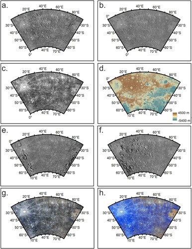
The BDR with 166 m/pixel resolution is the highest resolution globally available and the main mosaic used for mapping (Figure 1(a)). The BDR is constructed from images with an incidence angle close to 74°. A 250 m/pixel BDR mosaic produced during MESSENGER’s mission was also used for certain areas where the mosaic is more consistent, or has different illumination geometries, than the 166 m/pixel mosaic (Figure 1(b)).

Figure 1. Data used during mapping: a. Bulk data record (166 m/pixel) basemap, b. Bulk data record (250 m/pixel) basemap, c. Low incidence angle basemap, d. colour-keyed digital terrain model overlain with hillshade (Becker et al., 2016), e. High incidence west basemap, f. High incidence east basemap, g. colour basemap, and h. enhanced colour basemap (Denevi et al., 2018).

A grid of eight different basemaps showing the surface of the Debussy quadrangle.

2.2. Low incidence angle basemap

This mosaic at 166 m/pixel resolution is composed images captured close to solar noon. It was useful to identify albedo features and ejecta (Figure 1(c)).

2.3. Digital terrain model basemap

The digital terrain model helped to identify tectonic features. This has a resolution of 665 m/pixel and was derived from stereo images (Becker et al., 2016). It was displayed as colour-keyed elevation overlain by hill shaded relief during mapping (Figure 1(d)).

2.4. High incidence angle basemaps

High Incidence West/East mosaics with a resolution of 166 m/pixel were useful for identifying structures (Figure 1(e, f)).

2.5. Colour and enhanced colour basemap

We used two colour 665 m/pixel mosaics derived from the MDIS Wide Angle Camera. The colour base map (Figure 1(g)) uses 1000, 750, and 430 nm narrow-band filters in the red, green, and blue channels (Denevi et al., 2018). The enhanced colour basemap (Figure 1(h)) uses the 430, 750, and 1000 nm bands. It places the second principal component in the red, the first principal component in the green, and the ratio of 430/1000 nm bands in the blue channel (Denevi et al., 2018). We used it to map plains and surficial features.

3. Methods

3.1 Projection

The map uses a spheroid radius of 2,439,400 m, with a Lambert conformal conic projection (Lambert, 1772) with standard parallels at 30° and 58° S and a central meridian of 45° E.

3.2 Scale

The publication scale is 1:3 million, consistent with other post MESSENGER quadrangle maps features needed to be at least 3 km wide to be mappable; this forms an element at least 1 mm wide on the map. We used a mapping scale 2,000 times the basemap pixel scale (Tobler, 1987) so 1: ∼300,000 for the 166 m/pixel basemap and a streaming length (distance between vertices) of 900 m as this representing 0.3 mm at mapping scale (Tanaka et al., 2011).

3.3 Mapping strategy

We followed the mapping standards of the US Geological Survey (Tanaka et al., 2011), Planmap (Rothery & Balme, 2018), and those set out by the other 1:3 million scale quadrangle maps (e.g. Galluzzi et al., 2016; Wright et al., 2019). We first produced the linework for tectonic structures and crater rims, and then contacts between units. We converted the contacts into polygons, with attribute information applied relating to interpretation. Line styles represent both the type of feature and the relative certainty of the line’s location.

3.4 Contacts

The interface between units is known as a ‘contact’. In some cases, this occurs at a lobate scarp, but the majority of the boundaries are stratigraphic contacts. The type of boundary and the confidence in its location dictate the style of the line.

‘Certain’ contacts are unbroken lines, indicating clear, abrupt boundary and representing confidence in the precise location (±1 km) of the contact at the scale mapped and most commonly found at the edge of Smooth Plains, or at the boundary between crater floor material and its wall/central peak. ‘Approximate’ contacts are where we could not identify the exact location due to data quality or a gradual transition between units. Such contacts are usually found between Intercrater Plains and Intermediate Plains. Internal contacts occur within both Smooth plains and Intercrater Plains where the unit morphologies match the description but there is a distinct internal boundary, likely due to different generations of the same morphology.

3.5 Tectonic features

3.5.1 Lobate scarps

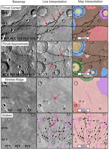
Thrusts faults typically manifest on the surface of Mercury as asymmetric lobate scarps (e.g. Watters et al., 1998). We drew linework at the break of slope at the base of the steeper side of the feature. The triangular teeth in the line symbol point towards the hanging wall. Levels of certainty reflect how clear the break in slope is; solid lines show clearly defined examples. Where the identification is uncertain, a dashed line is used (Figure 2). Faults without a clear direction are shown as a dashed line with no teeth.

Figure 2. Examples of linework for tectonic features, showing thrust faults, both certain and approximate represented by linework embellished with triangles, wrinkle ridges represented by pink linework and graben structures represented by linework embellished with circles (examples highlighted by red arrows). The background is the BDR basemap, with 30% transparency in line interpretation. The geology map has 40% transparency.

A grid of diagrams showing the different line styles of the structures the map.

3.5.2 Wrinkle ridges

Wrinkle ridges are identified by their usually symmetrical profile and lower relief than lobate scarps (e.g. Watters & Nimmo, 2010). We mapped these as a single continuous pink line placed over the crest. Due to their subtle appearance, they are represented by a solid line with no certainty levels applied (Figure 2).

3.5.3 Grabens

Grabens are the only extensional structures identified. They are manifest as negative relief (shown by shadows), linear structures. Whilst generally the width of a single line, some grabens in the Rembrandt impact basin are wider; here the linework traces the middle of the graben (Figure 2). A solid line is used where the location is confident, and dashed where uncertain.

4. Geological units

We divided the map into geological units. We continue to use the main units identified in the Mariner 10 and previous 1:3 million scale maps as they help understand the geological history within the quadrangle and allow compatibility with the other quadrangle maps. There are two principal types of unit on Mercury: crater materials and plains materials.

4.1 Craters

We mapped and classified craters within the quadrangle based on their size and degradation.

4.1.1 Crater outlines

We mapped rims of craters >5 km but <20 km with a single black outline with no unit assigned to them. We showed rims buried by ejecta from subsequent nearby impactors with a dot-dashed symbol. We mapped the rims of craters >20 km diameter with a solid line with double inwards ticks and their associated geologic materials were distinguished into units.

4.1.2 Degradation

In the majority of cases crater degradation reflects how long crater features (rim, ejecta, walls, floor, terraces) have been modified by subsequent smaller impacts and space weathering. The maps produced using Mariner 10 images and the global map use a 5-class system (Kinczyk et al., 2018, 2020; Spudis & Guest, 1988, Table 2, Figure 3). Several post-MESSENGER 1:3 million maps use a simplified 3-class system (e.g. Galluzzi et al., 2016, Table 1, Figure 4), with the aim of reducing the conflicts between degradation state and superposition relationships (because the rate of degradation is size dependent).

Figure 3. Examples of 5-class crater classification showing a progression from least degraded c5 to most degraded c1., c5 orange, c4 purple, c3 green, c2 blue, c1 light blue, red arrows point to example crater. The background is the BDR basemap, with 30% transparency in line interpretation. The geology map has 40% transparency.

A grid of diagrams showing the different crater degradation patch for the 5-class degradation system. The least degraded are c5 which have fresh ejecta and rays are symbolised in dark yellow, c4, which have lost their bright ejecta rays, are in purple. c3, where there are superposed craters and some degradation to ejecta and crater rims are in green. c2 craters have lost most of their terraces and only have a highly degraded central peak, if present, are symbolised in dark blue. c1 craters of which a highly degraded rim is the main feature to remain are illustrated in light blue.

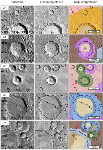
Figure 4. Examples of the 3-class system crater types: red arrows point at example craters. On the map interpretation panels, Yellow = C3 (least degraded), Green = C2 (moderately degraded), and Red = C1 (most degraded). The background is the BDR basemap, with 30% transparency in line interpretation. The geology map has 40% transparency.

A grid of diagrams showing the different crater degradation patch for the 3-class degradation system. C3, the freshest craters are in yellow. C2, where there are some superposing craters and features such as terraces are degraded in green. C1, where impact craters no longer show terraces of central peaks and have lost most of their ejecta, are shown in red.

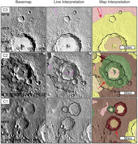
Table 1. 3-Crater Class system features (based on Galluzzi et al., 2016).

Crater class	Rim	Crater floor-wall boundary	Ejecta	Secondary craters	Superposed Craters
C3	Continuous and crisp	Crisp break, clearly defined	Continuous, highly textured	Clear secondary chains and sometimes crater rays	Rare
C2	Mostly continuous, but subdued	Gradational break, clearly defined	Continuous, but degraded (loss of distinct texture)		low to moderate density
C1	Subdued and discontinuous	subdued break and poorly defined	Discontinuous, and degraded		moderate to high density

Table 2. Description of 5 Class crater system based on (Kinczyk et al., 2020).

Class	Rays	Rim	Terraces	Floor-wall boundary	Ejecta	Secondary craters	Central peaks	Superposed craters
c5	Bright rays present	Clear, crisp, continuous	Crisp	Crisp break	Radially textured continuous	Well defined continuous field of crisp secondary craters	Crisp	None
c4	No Rays	Crisp, continuous	Crisp to slightly degraded	Crips break	Radially textured continuous	Well defined	Crisp	Rare
c3	-	Mostly Continuous, but showing degradation,	Most very degraded	Boundary subdued but still identifiable	Mostly continuous with some interruptions around the radius	Some but not continuous and highly degraded	Subdued	Low to moderate density
c2	-	Continuous to discontinuous degraded with a rounded appearance	Remnant in larger craters	Boundary indistinct unless embayed by lava in some areas	Discontinuous to absent	None	Rare central peak rings, heavily degraded	Moderate density
c1	-	Discontinuous degraded only slightly above surroundings	No wall terraces	No floor wall boundary	No deposit away from the rim, boundary unclear	None	No central peak rings	Moderate to high density

Wright et al. (2019) classified using both systems and produced two versions of their map. We likewise produced 3- and 5-class versions of our map (Main Map) where the degradation states of the craters are represented by their mapped ejecta and rim materials. We use the same convention as Wright et al. (2019), with a capitalised ‘C’ for the 3-class system (e.g. C1, C2, C3) and a lower case ‘c’ for the 5-class system (e.g. c1, c2, c3, c4, c5). Increasing degradation state usually corresponds to older craters in the stratigraphic order, but for both systems we found rare cases of more degraded craters superposed on (and hence younger than) less degraded craters. We attribute this to either: smaller craters degrading more rapidly than larger craters, or proximity to a younger impact whose ejecta has degraded the morphology of the nearest craters.

4.1.3 Crater floor material

4.1.3.1 Smooth crater floor material (scf)

Smooth material confined to crater floors. In fresh craters this is interpreted as representing ponding of impact melt (Daniels, 2018). In older craters this may be subsequent volcanic plains.

4.1.3.2 Hummocky crater floor material (hcf)

Rough textured crater floors, often with superposed small craters. These tend to occur in more degraded craters (Galluzzi et al., 2016).

4.2 Plains units

Outside of craters, we have followed previous maps of Mercury, (e.g. Galluzzi et al., 2016; Schaber & McCauley, 1980) by dividing the surface into plains with different textural features: Intercrater, Intermediate and Smooth Plains units.

4.2.1 Smooth plains (sp)

Smooth Plains are relatively flat, with few superimposed impact craters (Denevi et al., 2013). This is the youngest plains unit. It occurs as discrete patches with generally distinct boundaries and usually occupying low-lying areas such as within the Rembrandt impact basin. Smooth Plains tend to have a higher albedo and are spectrally redder in colour than Intercrater Plains (icp), however, this is not always the case. Older craters within Smooth Plains are infilled and/or embayed, whereas superposed craters retain a highly textured ejecta blanket. These plains are probably lava flows that have not been significantly degraded by subsequent cratering (Denevi et al., 2009; Head et al., 2008).

4.2.2 Intercrater plains (icp)

These plains gently undulating on scales of 10s to 100s of kilometres (Trask & Guest, 1975). Small (5–15 km) craters dominate their surfaces (Figure 5). The craters’ shallowness suggests that many are secondaries, although generally they cannot be linked to parent craters (Spudis & Guest, 1988; Whitten et al., 2014). Intercrater Plains are the most widespread plains on Mercury (Kinczyk et al., 2020; Murray et al., 1975; Strom et al., 2011; Whitten et al., 2014), and they have highly variable spectral properties and a wide range of craters sizes and all degradation stages. These are interpreted to be ancient lava flow fields significantly modified by subsequent impacts (Whitten et al., 2014).

Figure 5. Examples of the three different plains units on the BDR basemap. Red arrows point to units. The background is the BDR basemap, with 30% transparency in line interpretation. The geology map has 40% transparency.

A grid of diagrams showing the classification of plains units: Smooth plains that are very flat surfaces with few and small (<5 km) craters superposed are light pink. Intermediate plains, which have a higher density of small craters but still appear flat, are in dark pink. Intercrater plains, which are saturated with small craters and undulate, are symbolised in brown.

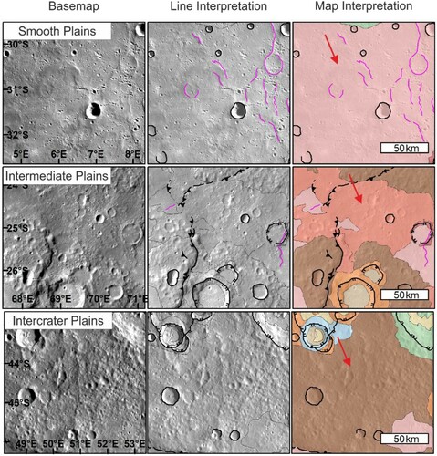
4.2.3 Intermediate plains (ip)

Intermediate Plains contrast with Smooth Plains by having a more undulating texture and more superimposed craters, many of which are subdued or mantled. Unit ip does not have a distinct boundary with underlying units (usually icp) but is less cratered than icp. The existence of the Intermediate Plains unit is controversial: Whitten et al. (2014) suggest they are not a distinct unit, but represent different levels of degradation of Intercrater Plains or Smooth Plains, and so not included in the global map (Kinczyk et al., 2020). The 1:3M maps so far produced see them as necessary in showing the whole variety of surface types. We map ip as a separate unit (Figure 5) and interpret them as an intermediate age of lava plains formation, consistent with previous 1:3M maps (e.g. Galluzzi et al., 2016; Wright et al., 2019).

4.3 Rembrandt-specific units

The Rembrandt impact basin has some noteworthy features within it and several different styles of ejecta. We elected to map these as basin-specific units. This is an approach adopted in maps of the Caloris basin (Fassett et al., 2009; McCauley et al., 1981; Guest & Greeley, 1983; Guzzetta et al., 2017; Mancinelli et al., 2016; Solomon et al., 2007; Trask & Guest, 1975) and also in previous maps of Rembrandt (Hynek et al., 2017; Semenzato et al., 2020). We preface Rembrandt-specific units with ‘Re’.

4.3.1 Hummocky unit (Reh)

Part of the basin floor of Rembrandt is uneven and mapped as a hummocky unit (Hynek et al., 2017; Semenzato et al., 2020; Watters et al., 2009). The edges of this unit are gradational. The unit is morphologically different from typical crater floor due to smooth undulating terrain between the discrete hummocks, which are 15–50 m high. The hummocky unit has a lower albedo than most of the Smooth Plains that cover much of the rest of the floor of Rembrandt. (Figure 6). This unit is interpreted to be part of the basin floor not covered over by subsequent lavas (Watters et al., 2009).

Figure 6. Examples of the Rembrandt-specific units. The background is the BDR basemap, red arrows point to particular unit. The background is the BDR basemap, with 30% transparency in line interpretation, geology map has 40% transparency.

A grid of diagrams showing the five units around Rembrandt. The hummocky material is rough, and relatively low albedo is symbolised by a lime green. The Massifs are blocks and mounds sticking out from the basin floor and symbolised in dark green. The Rim unit is a cliff on the edge of the impact basin, and that is symbolised by a mid-green. Ejecta around the basin which is rough but not lineated is symbolised a very light pastel green. Lineated ejecta unit undulates and has features that radiate away from the Rembrandt impact basin, and it is represented by a pastel green.

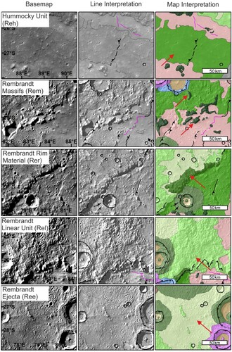
4.3.2 Rembrandt massifs (Rem)

These are blocky hills (up to 1 km high) protruding above the basin floor units Reh and sp (Figure 6). They lack strong fabric and we interpret these to be blocks of impact ejecta.

4.3.3 Rembrandt rim material (Rer)

This unit was first identified by Hynek et al. (2017). It comprises a series of massifs that make up part of the basin rim (predominantly on the northwest side) and lack strong radial feature. The outer contact is gradational and in some areas a basin-radial fabric begins to form. Rer is similar to the Caloris Montes unit which forms the elevated part of the Caloris basin rim (Fassett et al., 2009).

4.3.4 Rembrandt linear unit (Rel)

This unit is distinguished by surface texture radiating away from the basin in the form of ridges and troughs (Hynek et al., 2017; Watters et al., 2009; Whitten & Head, 2015). It includes blocky areas and smoother patches too small to map individually (Figure 6). We interpret this to be radiating ejecta, similar, and probably analogous, to the Van Eyck formation at Caloris (Fassett et al., 2009).

4.3.5 Rembrandt ejecta (Ree)

This unit comprises hills undulating at scales of tens of kilometres. It is smoother than icp, has a lower density of craters, and often contains flat ‘pools’ that look like filled craters (Figure 6).

4.4 Superficial units

Features that do not entirely obscure underlying units are mapped as superficial units. These are faculae (diffuse red patches interpreted to be explosive volcanic deposits; Gillis-Davis et al., 2009; Head et al., 2008), hollows (bright blue rimmed pits associated with volatile loss (Blewett et al., 2011)), crater chains (catenae), and bright ejecta rays (Braden & Robinson, 2013).

5. Correlation of map units

The stratigraphic column (Figure 7) summarises the inferred geological history of the quadrangle using the 5-class crater system. The formation ages of the plains units are based on global estimates (Byrne et al., 2016; Strom et al., 2011; Whitten et al., 2014). Within the map both Smooth Plains and Intermediate plains overprint Intercrater Plains, however the relationship between Intermediate Plains and Smooth Plains is not apparent. The crater ages are based on (Kinczyk et al., 2020). As noted in Section 4.1, crater degradation state usually correlates with stratigraphic position (with exceptions for some smaller craters).

Figure 7. Stratigraphic column describing the proposed temporal order of units and processes in the H-14 quadrangle. (sp: Smooth Plains, ip: Intermediate Plains, icp: Intercrater plains, Rer: Rembrandt Rim, Ree: Rembrandt Ejecta, Rem: Rembrandt Massif, Reh Rembrandt Hummocky material, Rel Rembrandt Linear unit), Eras from (Spudis & Guest, 1988; Banks et al., 2017).

The Figure is a stratigraphic column for the map showing the approximate relationships between the c5 craters and the units. Crater units c1 are the oldest and c5 the youngest. Intercrater plains match with the c1, with intermediate plains predating the smooth plains (which primarily form during the c2 and c3 formation), c4 and c5 craters postdate the plains formation.

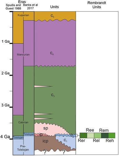
The map is dominated by the Intercrater plains unit. There is less Smooth or Intermediate plains than in the other quadrangles that have so far been published, these quadrangles include the extensive northern Smooth Plains which dominate the northern hemisphere (e.g. Denevi et al., 2013).

6. Summary

We have used data collected by the MESSENGER spacecraft to make the first geological map of the H-14 Debussy quadrangle on Mercury. We have mapped crater degradation using two schemes. The map is dominated by Intercrater plains and terrains related to the Rembrandt impact basin. We have distinguished an Intermediate plains unit, in agreement with other quadrangle maps.

Software

The basemaps were processed using USGS ISIS3, we used ESRI ArcMap 10.5 to produce the map, and the Map sheet was produced using CorelDraw.

Acknowledgements

The image data products used in this paper are publicly available from the Planetary Data System (PDS). MESSENGER data credited to NASA/Johns Hopkins University Applied Physics Laboratory/Carnegie Institute of Washington. Thank you to David Crown for reviewing the paper, and Giedrė Beconytė and Laura Guzzetta for reviewing the map sheets.

Disclosure statement

No potential conflict of interest was reported by the author(s).

Data availability statement

Digital copies of the shape files and basemaps can be found here: https://ordo.open.ac.uk/articles/dataset/Geological_map_data_for_the_H14_Debussy_quadrangle/14207174

Additional information

Funding

David Pegg was funded by the UK Science and Technology Facilities Council (STFC) under grant ST/R504993/1, the Open University’s Space Research Area and from European Commission Horizon 2020 Grant 776276 (Planmap). DAR and MJB received support from European Commission Horizon 2020 Grant 776276 (Planmap) for Mercury mapping. SJC is grateful for financial support from the French Space Agency CNES for her BepiColombo related work.

References

- Banks, M. E., Xiao, Z., Braden, S. E., Barlow, N. G., Chapman, C. R., Fassett, C. I., & Marchi, S. S. (2017). Revised constraints on absolute age limits for Mercury's Kuiperian and Mansurian stratigraphic systems. Journal of Geophysical Research: Planets, 122(5), 1010–1020.
- Becker, K. J., Robinson, M. S., Becker, T. L., Weller, L. A., Edmundson, K. L., Neumann, G. A., Perry, M. E., & Solomon, S. C. (2016). First global digital elevation model of Mercury. In Lunar and planetary science conference. No. 1903 (pp. 2959).
- Blewett, D. T., Chabot, N. L., Denevi, B. W., Ernst, C. M., Head, J. W., Izenberg, N. R., Murchie, S. L., Solomon, S. C., Nittler, L. R., McCoy, T. J., & Xiao, Z. (2011). Hollows on Mercury: MESSENGER evidence for geologically recent volatile-related activity. Science, 333(6051), 1856–1859. https://doi.org/https://doi.org/10.1126/science.1211681
- Braden, S. E., & Robinson, M. S. (2013). Relative rates of optical maturation of regolith on Mercury and the moon. Journal of Geophysical Research: Planets, 118(9), 1903–1914. https://doi.org/https://doi.org/10.1002/jgre.20143
- Byrne, P. K., Ostrach, L. R., Fassett, C. I., Chapman, C. R., Denevi, B. W., Evans, A. J., Klimczak, C., Banks, M. E., Head, J. W., & Solomon, S. C. (2016). Widespread effusive volcanism on Mercury likely ended by about 3.5 Ga. Geophysical Research Letters, 43(14), 7408–7416. https://doi.org/https://doi.org/10.1002/2016GL069412
- Daniels, J. (2018). Impact melt emplacement on mercury. Western Libraries Electronic Thesis and Dissertation Repository. 5657.
- De Hon, R. A., Scott, D. H., & Underwood Jr, J. R. (1981). Geologic map of the Kuiper (H-6) quadrangle of Mercury. United States Geological Survey, Geologic Investigations Series, Map I-1233.
- Denevi, B. W., Chabot, N. L., Murchie, S. L., Becker, K. J., Blewett, D. T., Domingue, D. L., Ernst, C. M., Hash, C. D., Hawkins, S. E., Keller, M. R., & Laslo, N. R. (2018). Calibration, projection, and final image products of MESSENGER’s mercury dual imaging system. Space Science Reviews, 214(1), 1–52. https://doi.org/https://doi.org/10.1007/s11214-017-0440-y
- Denevi, B. W., Ernst, C. M., Meyer, H. M., Robinson, M. S., Murchie, S. L., Whitten, J. L., Head, J. W., Watters, T. R., Solomon, S. C., Ostrach, L. R., & Chapman, C. R. (2013). The distribution and origin of smooth plains on Mercury. Journal of Geophysical Research: Planets, 118(5), 891–907. https://doi.org/https://doi.org/10.1002/jgre.20075
- Denevi, B. W., Robinson, M. S., Solomon, S. C., Murchie, S. L., Blewett, D. T., Domingue, D. L., McCoy, T. J., Ernst, C. M., Head, J. W., Watters, T. R., & Chabot, N. L. (2009). The evolution of Mercury’s crust: A global perspective from MESSENGER. Science, 324(5927), 613–618. https://doi.org/https://doi.org/10.1126/science.1172226
- Fassett, C. I., Head, J. W., Blewett, D. T., Chapman, C. R., Dickson, J. L., Murchie, S. L., Solomon, S. C., & Watters, T. R. (2009). Caloris impact basin: Exterior geomorphology, stratigraphy, morphometry, radial sculpture, and smooth plains deposits. Earth and Planetary Science Letters, 285(3-4), 297–308. https://doi.org/https://doi.org/10.1016/j.epsl.2009.05.022
- Galluzzi, V., Guzzetta, L., Ferranti, L., Di Achille, G., Rothery, D. A., & Palumbo, P. (2016). Geology of the Victoria quadrangle (H02), Mercury. Journal of Maps, 12(sup1), 227–238. https://doi.org/https://doi.org/10.1080/17445647.2016.1193777
- Gillis-Davis, J. J., Blewett, D. T., Gaskell, R. W., Denevi, B. W., Robinson, M. S., Strom, R. G., Solomon, S. C., & Sprague, A. L. (2009). Pit-floor craters on Mercury: Evidence of near-surface igneous activity. Earth and Planetary Science Letters, 285(3-4), 243–250. https://doi.org/https://doi.org/10.1016/j.epsl.2009.05.023
- Grolier, M. J., & Boyce, J. M. (1984). Geologic map of the Borealis region (H-1) of Mercury. United States Geological Survey, Miscellaneous Investigations Series. Map I–1660.
- Guest, J. E., & Greeley, R. (1983). Geologic map of the Shakespeare (H-3) quadrangle of Mercury. United States Geological Survey, Miscellaneous Investigations Series. Map I–1408.
- Guzzetta, L., Galluzzi, V., Ferranti, L., & Palumbo, P. (2017). Geology of the Shakespeare quadrangle (H03), Mercury. Journal of Maps, 13(2), 227–238. https://doi.org/https://doi.org/10.1080/17445647.2017.1290556
- Hawkins, S. E., Boldt, J. D., Darlington, E. H., Espiritu, R., Gold, R. E., Gotwols, B., Grey, M. P., Hash, C. D., Hayes, J. R., Jaskulek, S. E., & Kardian, C. J. (2007). The Mercury dual imaging system on the MESSENGER spacecraft. Space Science Reviews, 131(1), 247–338. https://doi.org/https://doi.org/10.1007/s11214-007-9266-3
- Head, J. W., Murchie, S. L., Prockter, L. M., Robinson, M. S., Solomon, S. C., Strom, R. G., Chapman, C. R., Watters, T. R., McClintock, W. E., Blewett, D. T., & Gillis-Davis, J. J. (2008). Volcanism on Mercury: Evidence from the first MESSENGER flyby. Science, 321(5885), 69–72. https://doi.org/https://doi.org/10.1126/science.1159256
- Hynek, B. M., Robbins, S. J., Mueller, K., Gemperline, J., Osterloo, M. K., & Thomas, R. (2017). Unlocking Mercury's geological history with detailed mapping of Rembrandt basin: Year 3. In Third planetary data workshop and the planetary geologic mappers annual meeting. Vol. 1986 (pp. 7098).
- Kinczyk, M. J., Prockter, L. M., Byrne, P. K., Susorney, H. C., & Chapman, C. R. (2020). A morphological evaluation of crater degradation on Mercury: Revisiting crater classification with MESSENGER data. Icarus, 341, 113637. https://doi.org/https://doi.org/10.1016/j.icarus.2020.113637
- Kinczyk, M. J., Prockter, L. M., Denevi, B. W., Ostrach, L. R., & Skinner, J. A. (2018). A global geological map of Mercury. In Mercury: Current and Future Science of the Innermost Planet (Vol. 2047, pp. 6123.
- King, J. S., & Scott, D. H. (1990). Geologic map of the Beethoven (H-7) quadrangle of Mercury. United States Geological Survey, Miscellaneous Investigations Series. Map I–2048.
- Lambert, J. H. (1772). Anmerkungen und Zusätze zur Entwerfung der Land-und Himmelscharten. Hrsg. von A.
- Malliband, C. C., Rothery, D. A., Balme, M. R., & Conway, S. J. (2020). 1:3M Geological Mapping of the Derain (H-10) quadrangle of Mercury. British Planetary Science Conference, 2020, 79.
- Man, B., Rothery, D. A., Balme, M. R., & Conway, S. J. (2020). Geological Mapping of the Neruda Quadrange (H13) of Mercury. Annual Meeting of Planetary Geologic Mappers. P. 7028.
- Mancinelli, P., Minelli, F., Pauselli, C., & Federico, C. (2016). Geology of the raditladi quadrangle, Mercury (H04). Journal of Maps, 12(sup1), 190–202. https://doi.org/https://doi.org/10.1080/17445647.2016.1191384
- McCauley, J. F., Guest, J. E., Schaber, G. G., Trask, N. J., & Greeley, R. (1981). Stratigraphy of the Caloris basin, Mercury. Icarus, 47(2), 184–202. https://doi.org/https://doi.org/10.1016/0019-1035(81)90166-4
- McGill, G. E., & King, E. A. (1983). Geologic map of the Victoria (H-2) quadrangle of Mercury. United States Geological Survey, Miscellaneous Investigations Series. Map I–1409.
- Murray, B. C., Strom, R. G., Trask, N. J., & Gault, D. E. (1975). Surface history of Mercury: Implications for terrestrial planets. Journal of Geophysical Research, 80(17), 2508–2514. https://doi.org/https://doi.org/10.1029/JB080i017p02508
- Prockter, L. M., Ernst, C. M., Denevi, B. W., Chapman, C. R., Head, J. W., Fassett, C. I., Merline, W. J., Solomon, S. C., Watters, T. R., Strom, R. G., & Cremonese, G. (2010). Evidence for young volcanism on Mercury from the third MESSENGER flyby. Science, 329(5992), 668–671. https://doi.org/https://doi.org/10.1126/science.1188186
- Rothery, D. A., & Balme, M. R. (2018). Planmap Mapping Standards Document. Plan Map. https://wiki.planmap.eu/display/public/D2.1-public
- Schaber, G. G., & McCauley, J. F. (1980). Geologic map of the Tolstoj (H-8) quadrangle of Mercury. United States Geological Survey, Miscellaneous Investigations Series, Map I-1199.
- Semenzato, A., Massironi, M., Ferrari, S., Galluzzi, V., Rothery, D. A., Pegg, D. L., Pozzobon, R., & Marchi, S. (2020). An integrated geologic map of the Rembrandt basin, on Mercury, as a starting point for stratigraphic analysis. Remote Sensing, 12(19), 1–33. https://doi.org/https://doi.org/10.3390/rs12193213
- Solomon, S. C., McNutt, R. L., Gold, R. E., & Domingue, D. L. (2007). MESSENGER mission overview. Space Science Reviews, 131(1-4), 3–39. https://doi.org/https://doi.org/10.1007/s11214-007-9247-6
- Spudis, P. D., & Guest, J. E.. (1988). Stratigraphy and geologic history of Mercury. In Mercury (pp. 118–164).
- Spudis, P. D., & Prosser, J. G. (1984). Geologic map of the Michelangelo (H-12) quadrangle of Mercury. United States Geological Survey, Miscellaneous Investigations Series. Map I-1659.
- Strom, R. G., Banks, M. E., Chapman, C. R., Fassett, C. I., Forde, J. A., Head III, J. W., Merline, W. J., Prockter, L. M., & Solomon, S. C. (2011). Mercury crater statistics from MESSENGER flybys: Implications for stratigraphy and resurfacing history. Planetary and Space Science, 59(15), 1960–1967. https://doi.org/https://doi.org/10.1016/j.pss.2011.03.018
- Strom, R. G., Malin, M. C., & Leake, M. A. (1990). Geologic map of the Bach (H-15) quadrangle of Mercury. United States Geological Survey, Miscellaneous Investigations Series, Map I-2015.
- Tanaka, K. L., Skinner, J. A., & Hare, T. M. (2011). Planetary Geologic Mapping Handbook – 2011. Abstracts of the Annual Meeting of Planetary Geologic Mappers. https://ntrs.nasa.gov/archive/nasa/casi.ntrs.nasa.gov/20100017213.pdf
- Tobler, W. (1987). Measuring spatial resolution. In: Proceedings of the land resource information systems conference. p. 12–16.
- Trask, N. J., & Dzurisin, D. (1984). Geologic map of the Discovery (H-11) quadrangle of Mercury. United States Geological Survey, Miscellaneous Investigations Series. Map I-1658.
- Trask, N. J., & Guest, J. E. (1975). Preliminary geologic terrain map of Mercury. Journal of Geophysical Research, 80(17), 2461–2477. https://doi.org/https://doi.org/10.1029/JB080i017p02461
- Watters, T. R., Head, J. W., Solomon, S. C., Robinson, M. S., Chapman, C. R., Denevi, B. W., Fassett, C. I., Murchie, S. L., & Strom, R. G. (2009). Evolution of the Rembrandt impact basin on Mercury. Science, 324(5927), 618–621. https://doi.org/https://doi.org/10.1126/science.1172109
- Watters, T. R., & Nimmo, F.. (2010). The tectonics of Mercury. In Planetary tectonics (Vol. 11, pp.15–80). Cambridge: Cambridge University Press.
- Watters, T. R., Robinson, M. S., & Cook, A. C. (1998). Topography of lobate scarps on Mercury: New constraints on the planet's contraction. Geology, 26(11), 991–994. https://doi.org/https://doi.org/10.1130/0091-7613(1998)026<0991:TOLSOM>2.3.CO;2
- Whitten, J. L., & Head, J. W. (2015). Rembrandt impact basin: Distinguishing between volcanic and impact-produced plains on Mercury. Icarus, 258, 350–365. https://doi.org/https://doi.org/10.1016/j.icarus.2015.06.022
- Whitten, J. L., Head, J. W., Denevi, B. W., & Solomon, S. C. (2014). Intercrater plains on Mercury: Insights into unit definition, characterization, and origin from MESSENGER datasets. Icarus, 241, 97–113. https://doi.org/https://doi.org/10.1016/j.icarus.2014.06.013
- Wright, J., Rothery, D. A., Balme, M. R., & Conway, S. J. (2019). Geology of the Hokusai quadrangle (H05), Mercury. Journal of Maps, 15(2), 509–520. https://doi.org/https://doi.org/10.1080/17445647.2019.1625821