The spatial relationship between patterns of disappeared streams and residential development in Portland, Oregon, USA

ABSTRACT

Disappeared streams are streams that have been buried, removed, or moved as part of the urbanization process. We identified disappeared streams in the Portland, Oregon metropolitan area using historical topographic maps for four time periods, and related them to the history of urban development. The historical maps were used to identify streams visible in older maps but not shown in a more recent version. From 1852 to 1895, 15% of streams disappeared, but the majority of streams disappeared between 1896 and 1953 (65%). This trend continued mainly in suburban areas after 1954 with 12% of streams being removed from 1954 to 1989 and 8% from 1990 to 2017. Stream disappearance can be linked to residential development and prior conversion of land for agriculture depending on the area and time period. Mapping disappeared streams can help urban spatial planners identify where stream daylighting or restoration could be targeted.

KEYWORDS:

• Disappeared streams
• geographic information systems (GIS)
• land use
• historical topographic maps
• urbanization
• watershed

1. Introduction

Disappeared streams are streams that have been buried, removed, or moved as part of the urbanization process. Throughout human history, streams were rerouted into pipes and tunnels (buried) as population grew and city growth increased impervious surface areas (Brown et al., 2018; Chang et al., 2020; Hopkins & Bain, 2018; Napieralski & Welsh, 2016). Urban streams have also been altered to limit flooding (Abbott, 1994) and provide building sites for homes and businesses (Willingham, 1983). Burying or otherwise removing streams can have a number of negative impacts, including increased peak flow and reduced baseflow (Chang, 2007), increased pluvial flooding (Bae & Chang 2019; Houng & Pathirana, 2013; Rosenzweig et al., 2018), and damage to aquatic ecosystems (Stammler et al., 2013). Because of their important roles in the urban environment, it is essential to know the location of urban streams and their changes over time in relation to urbanization.

A number of researchers have mapped disappeared streams using geographic information systems (GIS). Elmore and Kaushal (2008) mapped the locations of disappeared streams within a major tributary of the Chesapeake Bay using high-resolution aerial photos and land cover data paired with a 10m resolution Digital Elevation Model (DEM). They found that while 20% of all streams were buried, small streams were more likely to be buried than larger streams. They suggest multiple explanations, including the higher cost of burying larger streams and the perennial nature of larger streams compared to smaller streams. Similarly, others have mapped disappeared streams in Detroit, Michigan, comparing the amount removed in the cities of Ann Arbor and Warren while exploring the concept of urban stream deserts (Napieralski et al. 2015; Napieralski & Carvalhaes, 2016; Napieralski & Welsh, 2016). Disappeared streams have been mapped in conjunction with sewage lines in Pittsburgh, Pennsylvania (Hopkins & Bain, 2018), and with a focus on land cover changes in the Lake Thunderbird watershed in Central Oklahoma (Julian et al., 2015). Mapping urban stream burial can reveal the history of urbanization practices and subsequent impact on urban hydrology (Napieralski, 2019) but also guide city design and planning (Napieralski, 2020).

While low-impact development or best management practices can be used to lower the hydrologic impact of stream removal, the natural flow cannot be fully renewed to the stream’s original state without stream restoration (Askarizadeh et al., 2015). Stream restoration has positive impacts on hydrology, reducing peak flow and sediment delivery (Ahilan et al. 2018) while increasing house sales prices (Netusil et al., 2019). For stream restoration efforts to be effective, we first need to know where and when streams disappeared and how the history of land development is associated with stream disappearance. Thus, this study examines the spatiotemporal pattern of disappeared streams in the Portland (Oregon) Metropolitan area since 1852 and has two main objectives: (1) Map disappeared streams for four time periods (1852 - 1895, 1896 - 1953, 1953 - 1989, and 1990–2017) and (2) Relate housing development to stream disappearance.

2. Development history and study area

Many stream networks have been moved or buried due to Portland's urban development. Founded in 1851, the city initially built its economy as a shipping hub for the region (Gibson & Abbott, 2002). Portland experienced a large wave of development in the early twentieth century because of a boom in population growth following the Lewis and Clark Centennial Exposition in 1905. During the Great Depression, the city received federal aid for highway construction and built a new airport, resulting in the loss of streams and wetlands. World War II saw many workers move to the area to work in the emerging shipbuilding industry (Gibson & Abbott, 2002). As it did elsewhere in the country, 1950s suburbanization resulted in a home-building boom in the Portland metropolitan area. After a period of economic stagnation in the 1960s, the metropolitan area experienced continued growth from the 1970s until the present as residents moved back into old neighborhoods as well as the expanding suburbs.

The Columbia River, Willamette River, and Johnson Creek have a history of flooding, with notable Portland area destructive floods occurring in 1861, 1894, 1948, and 1972 ( U.S. Army Corp of Engineers, 1973; Willingham, 1983). Eight recorded major floods of the Willamette River and four of the Columbia River occurred by 1936 with the great flood of 1894 being the most significant. The United State Flood Control Act of 1936 sponsored projects to reduce flooding across the United States, which included stream channelization and the construction of floodwalls, levees, dams, and reservoirs. For example, historic wetlands and floodplains were filled in and natural streams were straightened in the Johnson Creek watershed during the Works Progressive Administration era in the 1930s, which resulted in the loss of meandering streams. The modifications of natural channels increased flood risk in low lying areas along the Johnson Creek (Chang et al. 2021; Fahy et al., 2019; Hong & Chang, 2020).

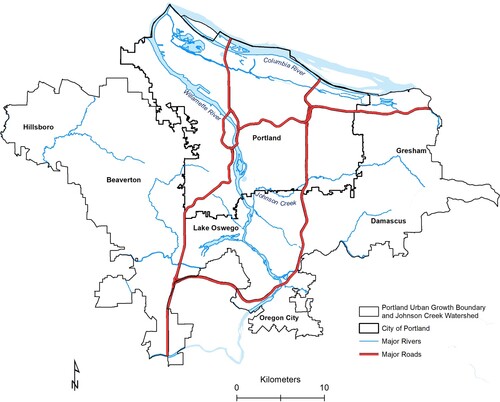
The study site encompasses the area within the Portland urban growth boundary combined with the Johnson Creek watershed boundary (Figure 1). The Portland urban growth boundary was established in 1973, and limits development outside the boundary (Abbott, 1994). While the urban growth boundary has encouraged dense development within the boundary and limited sprawl, the boundary has expanded about three dozen times to accommodate increasing population and employment growth by the regional government.

Figure 1. Map of the Portland metropolitan region with major rivers and streams.

General Map of Portland Urban Growth Boundary and Johnson Creek Watershed Boundary with major rivers, roads, City of Portland boundary depicted by different colors.

3. Materials and methods

Historical topographic maps were used to locate both where and when streams disappeared. The four periods studied, based on the availability of historical United States Geological Survey (USGS) georeferenced topographic maps, were 1852–1895, 1896–1953, 1954–1990, and 1990–2017. The range of time periods was necessary because the entire area of interest was not mapped in the same year. The 1852 map was the exception as it was not a USGS topographic map. This hand-drawn map dates from the founding of the city. Although it does not encompass the entire area of interest, it does show notable streams that were disappeared before the first USGS topographic map of the area was created. This map thus needed to be georeferenced before it could be used. Scale varied across the hand-drawn 1852 map, making any assessment of positional accuracy difficult at best. Disappeared streams in the 1896–1916 period were digitized from the topographic maps with a map scale of 1:62,500 while the topographic maps used for the 1954, 1990, and 2017 periods had a scale of 1:24,000. The smaller scale (1:62,500) maps likely had fewer features represented, and were certainly less accurate than the larger scale maps. Also, earlier maps, which relied on plane table surveying (1896-1916) where maps were drawn in the field from a high vantage point with a sighting device, are likely less accurate than those that used aerial photos to survey (1954, 2017).

Historical and current (USGS) topographic maps were downloaded from the TopoView website (Garrity, n.d.) for the study area. Table 1 shows the digital raster graphics (DRG) used within this study and their scale. Large-scale Digital Line Graphs (DLG) of hydrography lines, available from 1975 to 1990, were obtained from the USGS Earth Explorer website (US Geological Survey, 2020) in either native or Spatial Data Transfer Standard format and then converted to shapefile format using the DLG2SHP freeware program (Kerski, 2020). Both the topographic maps and DLGs were transformed into a common projected coordinate system (UTM, NAD83) using ArcMap 10.7.1 (ESRI, 2020). Both DLGs and DRGs were used as guides to help identify locations on the USGS topographic maps where streams were visible in historical maps but were not visible in more recent maps, representing disappeared streams. Each stream location was on-screen digitized using ArcMap 10.7.1.

Table 1. Sources and descriptions of maps.

Map name	Year	Method	Scale	Source
Location of streams (1852)
Portland	1852	unknown	unknown	City of Portland Archives
Location of streams (1896-1916)
Portland	1905	Surveyed in 1896	1:62500	USGS
Oregon City, Boring	1914	Surveyed in 1911–1912	1:62500	USGS
Tualatin	1915	Surveyed in 1915	1:62500	USGS
Troutdale	1918	Surveyed in 1916	1:62500	USGS
Location of streams (1954)
Camas	1954	Aerial photos and planetable survey in 1951, field check in 1954	1:24000	USGS
Damascus	1954	Aerial photos in 1952, field check in 1954	1:24000	USGS
Gladstone, Linnton	1954	Aerial photos, stereioplanisgraph in 1952, field check in 1954	1:24000	USGS
Mount Tabor	1954	Aerial photos, planetable survey, photogrammetric methods in 1951-1952, field check in 1954	1:24000	USGS
Lake Oswego, Sandy	1954	Aerial photos, planetable survey, photogrammetric methods in 1952, field check in 1954	1:24000	USGS
Portland, Vancouver	1954	Aerial photos, planetable survey, photogrammetric methods in 1951, field check in 1954	1:24000	USGS
Sauvie Island	1954	Aerial photos, planetable survey, photogrammetric methods in 1951, topo 1953–54	1:24000	USGS
Location of streams (1982-1996)
Linnton	1990	Aerial photos in 1952, revised 1990, edited in 1995	1:24000	USGS
Mount Tabor	1990	Aerial photos in 1951-1952, revised 1990, edited in 1995	1:24000	USGS
Oregon City	1982	Aerial photos in 1955-1974, 1981, edited in 1982	1:100000	USGS
Beaverton	1984	Aerial photos in 1981, edited In 1984	1:24000	USGS
Portland, Sauvie Island, Vancouver	1990	Aerial photos in 1951, Revised in 1990, edited in 1995	1:24000	USGS
Camas	1993	Aerial photos in 1951, revised in 1993, field checked in 1994, edited in 1996	1:24000	USGS
Location of streams (2014-2017)
Damascus, Gladstone, Lake Oswego, Linton, Mount Tabor, Portland, Sandy, Sauvie Island, Camas	2017	Imagery 2014	1:24000	USGS

After the disappeared streams were identified, each location was compared against a high resolution (0.15m) aerial photo from 2013 and also compared to the Regional Land Information System (RLIS) stream routes layer obtained from the Portland Metro Data Resource Center in 2003 (Oregon Metro, 2020). RLIS stream route data includes both existing streams and buried streams, but it does not identify type within its attributes. Thus, the aerial photo was used to validate that an identified stream disappeared. Streams that were re-routed were also identified as disappeared streams.

NHDplus hydrologic geospatial data layers were used for Hydrologic Unit Code (HUC) 12 watershed boundaries, as well as water body areas, which were used to show the major rivers in the study area (USGS, 2017). The Federal Emergency and Management Agency (FEMA) 100-year (1 percent annual chance) National Flood Hazard Layer (NFHL) representing floodplains was obtained from the NFHL ArcGIS Viewer.

The year that a building was constructed was obtained from RLIS tax lot data. Tax lots that intersected disappeared streams were selected and then the average and oldest year of building construction for each disappeared stream segment using the spatial join tool in ArcMap 10.7.1. We used both average and oldest year built since the former represents neighborhood age while the latter indicates the initial stage of development. The intersect tool (ArcMap 10.7.1) was used to create points where the disappeared streams intersected the boundaries of Portland’s Census Block Groups (CBG). Subsequently, the Split line at point tool was used to split each disappeared stream by CBG to calculate the stream density (m/km²). Stream density was calculated by dividing the total length of disappeared streams in each CBG by the area of that CBG.

4. Results and discussion

The initial 15% of stream length loss documented by this study occurred before the first USGS topographic maps were released. This accounts only for stream loss in the city of Portland as covered by the 1852 map, but most of the study area was sparsely populated prior to the twentieth century. Portland's population grew from 46,385 inhabitants in 1890–301,815 inhabitants in 1930 (Abbott, 1994). The surrounding regions within Portland's urban growth boundary did not witness the same amount of population growth as Portland in the same time frame (Abbott, 1994). The oldest houses still in existence (built starting in 1879) adjacent to disappeared streams in the study area are located in downtown Portland (Figure 2). The majority (65%) of identified stream length loss occurred between the years 1896–1953. Many houses built on these disappeared streams were likely constructed many years after the stream was removed. A possible explanation is that the stream was first removed for agriculture, and the same land was later developed into housing (Han et al., 2020; Julian et al., 2015). A 1908–1910 report from the Bureau of Labor Statistics confirmed the prevalence of agriculture and fruit orchards in Gresham, Beaverton, and Hillsboro (Hoff, 1911). The City of Damascus, Oregon, was founded in 1867 and was incorporated into the Portland Urban Growth Boundary in 2004. However, most of the streams disappeared in Damascus were already removed before 1954. In contrast, in Lake Oswego and along the Columbia River, streams disappeared from 1990 to 2017, likely associated with new infill commercial and residential development.

Figure 2. Map of disappeared streams symbolized by the oldest house construction date in the proximity of the former stream locations.

Map of Portland Urban Growth Boundary and Johnson Creek Watershed Boundary with disappeared streams symbolized by different colors associated with the oldest house construction date on the disappeared stream.

Suburban growth heightened from 1970 to the present within Portland's urban growth boundary. For example, the City of Gresham’s population increased by 229% from 1970 to 1980 and 107% from 1980 to 1990 and the City of Lake Oswego’s population increased by 54% and 36%, respectively, during the same period. The City of Beaverton’s population increased by 72% from 1970 to 1980 and 67% from 1980 to 1990, while the City of Portland’s population decreased 3% and grew 19%, respectively, during the same period (US Bureau of Census, 1992). Population growth outside of urban core likely led to development that covered or moved streams that were identified as disappeared between 1954-1989. Many of the streams disappeared after 1954 are in the western suburbs of the metropolitan area.

The oldest year when a house was built (Figure 2) near a disappeared stream is an indication of when an area was first developed, and the average house age (Figure 3) is an indication of when the area had a higher development level and house density. Most disappeared streams (68%) intersected parcels with a building that was constructed between the years 1896–1953. However, most buildings (52%) adjacent to disappeared streams were constructed between 1954–1989. Figure 4 shows an example of a disappeared stream with houses symbolized by the year of construction. The houses adjacent to the disappeared streams were built during the same time period when the stream was removed. New houses were built in subsequent years on top of historical streams (now disappeared streams). The highest density of disappeared streams occurred in areas where the average house was constructed between 1954 and 1989. However, the most recent development period (1990-2017) has a low density of disappeared streams (Figure 5). This low density of disappeared streams is likely attributed to either new stormwater management practices that minimize the alteration of existing streams or stream restoration efforts that result in daylighting covered streams (Fahy & Chang, 2019). There are many potential benefits of daylighting urban streams since they provide multiple ecosystem services (Palmer & Ruhi, 2019; Wolch et al., 2014; Yeakley et al., 2016). Streams in urban environments reduce nutrient pollution (Beaulieu et al., 2015), support wildlife and biodiversity in and around the streams (Meyer et al., 2007), and offer aesthetic value to residents and visitors (Kenney et al., 2012).

Figure 3. Map of disappeared streams symbolized by the average house construction date in the proximity of the former stream locations.

Map of Portland Urban Growth Boundary and Johnson Creek Watershed Boundary with disappeared streams symbolized by different colors associated with the average house construction date on the disappeared stream.

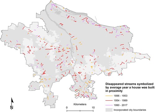
Figure 4. A high-resolution aerial photo showing examples of houses that were built in the proximity of a disappeared stream in the City of Portland, Oregon.

A map showing one disappeared stream in a neighborhood and different houses symbolized by the house construction date. Below the legend is three historic topographic maps of the same area showing how the stream disappeared over time.

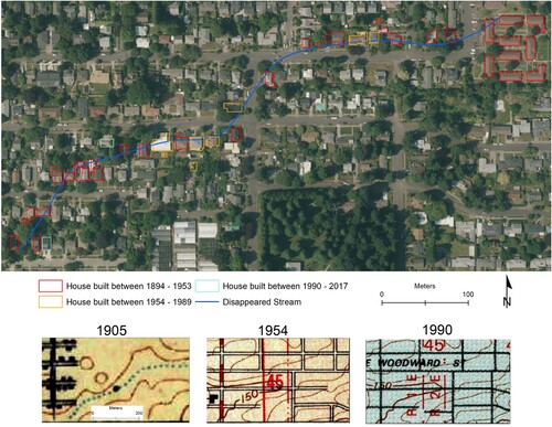
Figure 5. Density of streams per census block group (m of stream/km²).

Map of Portland Urban Growth Boundary and Johnson Creek Watershed Boundary with circles ranging in sizes according to the density of disappeared streams per census block group (m of stream/km2). The color of the census block groups represent the average house construction date where light blue is oldest (1896-1953), and the darkest blue is more recent (1990-2017).

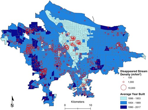
The density of disappeared streams in the study area (212 m/km²) exceeded rates calculated for other cities. Cities in Michigan, for example, ranged from 75 m/km² (Flint) to 153 m/km² (Ann Arbor) (Napieralski & Welsh, 2016). Notably, the density of disappeared streams (131 m/km²) identified from the oldest maps in this study (1852 to 1896-1916), was similar to the cities in Michigan. Both the maps in the Michigan study and the 1896–1916 maps used in this study were created at a 1:62,500 scale, which likely did not include smaller streams. The maps used to digitize the streams in the other periods within this study were digitized at a 1:24,000 scale, which likely showed additional streams within the study area. This map scale difference may explain the higher disappeared stream density over time.

5. Conclusions

Using historical topographic maps can be useful to study disappeared streams from urbanization over time. By relating stream disappearance to the year of building construction near disappeared streams, this study found that streams disappeared well before buildings were constructed, possibly due to agricultural land development, as indicated by the expansion of farmlands in the region. With the comprehensive collection of scanned and georeferenced topographic maps available from the USGS encompassing the twentieth century, it is possible to replicate the methodology used in this article for other cities. Depending on the development history of an urban area, using multiple periods of maps may help both identify a higher number of disappeared streams and understand the stream removal process over the twentieth century. The age of houses in proximity to where streams disappeared can offer important historical context of when and why a stream was lost.

There are some limitations of the current study. These limitations stem from primarily relying on the USGS historical topographic maps created after some of the initial development in Portland had occurred. An earlier, non-USGS topographic map did not cover the entire study region. As a result, the current approach is likely to have underestimated the lengths of disappeared streams for early development periods. Additionally, while the USGS topographic maps are good sources to describe what happened to urban streams, they do not provide answers as to why streams were rerouted or culverted. Thus, future studies can take advantage of using other archival information such as council planning minutes, stream engineering project design, and historic photographs. Together with USGS topographic maps, such supplementary information can enrich our understanding of the social and cultural context of urban streams removal processes.

The findings of the study have implications for spatial and environmental planning of the city. City planners and developers can learn from the history of disappeared streams and incorporate streams into their planning to limit ecological damage. Disappeared streams’ locations can be useful to identify areas where stream daylighting and ecological stream restoration may be possible. Areas of cities with disappeared streams may be less resilient to extreme weather events such as flooding since water flows into low-lying old channel areas when water levels increase (Chang et al., 2020). Thus, original hydrologic networks are beneficial for city climate resilience planning with their relationship with green spaces (Napieralski, 2020).

Software

Data creation including digitizing disappeared streams and cartographic design was done using ArcMap 10.7.1.

Acknowledgments

Funding for this project was provided by the Economics Internship Award from the Reed Institute. Additional support was provided by the U.S. National Science Foundation under Award number SES 1444755. We appreciate Dr. Jacob Napieralski, Dr. Martin Dodge, Dr. Giedre Beconyte and Editors Dr. Fleur Visser and Dr. Mike Smith for their careful review of our manuscripts. Views expressed are our own and do not necessarily reflect those of the sponsoring agencies.

Disclosure statement

No potential conflict of interest was reported by the author(s).

Data Availability Statement

The USGS topographic maps are available at https://ngmdb.usgs.gov/topoview/.

Regional Land Information System (RLIS) stream routes layer and parcel layer are available at the Oregon Metropolitan RLIS Discovery system https://gis.oregonmetro.gov/. The digitized disappeared stream GIS data that support the findings of this study are available at https://github.com/greggreg1/PDX_Disappeared_Streams.

Additional information

Funding

This work was supported by NSF: [Division of Chemical, Bioengineering, Environmental and Transport Systems (CBET), Grant Number 1444755, Urban resilience to extreme weather related events]; Reed College.

References

- Abbott, C. (1994). Settlement patterns in the Portland region: A historical overview. Portland Regional Planning History. Available at: http://archives.pdx.edu/ds/psu/14628.
- Ahilan, S., Guan, M., Sleigh, A., Wright, N., & Chang, H. (2018). The influence of floodplain restoration on flow and sediment dynamics in an urban river. Journal of Flood Risk Management, 11(S2), S986–S1001.
- Askarizadeh, A., Rippy, M. A., Fletcher, T. D., Feldman, D. L., Peng, J., Bowler, P., Mehring, A. S., Winfrey, B. K., Vrugt, J. A., AghaKouchak, A., Jiang, S. C., Sanders, B. F., Levin, L A. , Taylor, S., & Grant, S. B. (2015). From rain tanks to catchments: Use of low-impact development to address hydrologic symptoms of the urban stream syndrome. Environmental Science & Technology, 49(19), 11264–11280.
- Bae, S., & Chang, H. (2019). Urbanization and floods in the Seoul metropolitan area of South Korea: What old maps tell us. International Journal of Disaster Risk Reduction, 37, 101186.
- Beaulieu, J. J., Golden, H. E., Knightes, C. D., Mayer, P. M., Kaushal, S. S., Pennino, M. J., Arango, C. P., Balz, D. A., Elonen, C. M., Fritz, K. M., & Hill, B. H. (2015). Urban stream burial increases watershed-scale nitrate export. PLoS One, 10(7), e0132256.
- Brown, A. G., Lespez, L., Sear, D. A., Macaire, J. J., Houben, P., Klimek, K., Brazier, R. E., Van Oost, K., & Pears, B. (2018). Natural vs anthropogenic streams in Europe: History, ecology and implications for restoration, river-rewilding and riverine ecosystem services. Earth-Science Reviews, 180, 185–205.
- Chang, H. (2007). Comparative streamflow characteristics in urbanizing basins in the Portland metropolitan area, oregon, USA. Hydrological Processes, 21(2), 211–222.
- Chang, H., Eom, S., Yasuyo, M., & Bae, D. (2020). Land use change, extreme precipitation events, and flood damage in South Korea: A spatial approach. Journal of Extreme Events, 07((03|3)), 2150001.
- Chang, H., Yu, D., Markolf, S., Hong, C., Eom, S., Song, W., & Bae, D. (2021). Understanding urban flood resilience in the anthropocene: A social-ecological-technological systems (SETS) learning framework. Annals of the American Association of Geographers, 111(3), 837–857.
- Earth System Research Institute (ESRI). (2020). ArcMap 10.7. Redland, CA.
- Elmore, A. J., & Kaushal, S. (2008). Disappearing headwaters: Patterns of stream burial due to urbanization. Frontiers in Ecology and the Environment, 6(6), 308–312.
- Fahy, B., Brenneman, E., Chang, H., & Shandas, V. (2019). Spatial analysis of urban flooding and extreme heat hazard potential in portland, OR. International Journal of Disaster Risk Reduction, 39, 101117.
- Fahy, B., & Chang, H. (2019). Effects of stormwater Green infrastructure on watershed outflow: Does spatial distribution matter? International Journal of Geospatial and Environmental Research, 6(1), Article 5.
- Garrity, C. (n.d.). TopoView: USGS. Retrieved August 02, 2020, from https://ngmdb.usgs.gov/topoview/.
- Gibson, K., & Abbott, C. (2002). Portland, Oregon. Cities, 19(6), 425–436.
- Han, L., Xu, Y., Deng, X., & Li, Z. (2020). Stream loss in an urbanized and agricultural watershed in China. Journal of Environmental Management, 253, 109687.
- Hoff, O. P. (1911). Fourth Biennial Report of the Bureau of Labor Statistics and Inspector of Factories and Workshops of the State of Oregon From October 1, 1908, to September 30, 1910.
- Hong, C.-Y., & Chang, H. (2020). Residents' perception of flood risk and urban stream restoration using multi-criteria decision analysis. River Research and Applications, 36(10), 2078–2088.
- Hopkins, K. G., & Bain, D. (2018). Research note: Mapping spatial patterns in sewer age, material, and proximity to surface waterways to infer sewer leakage hotspots. Landscape and Urban Planning, 170, 320–324.
- Huong, H. T. L., & Pathirana, A. (2013). Urbanization and climate change impacts on future urban flooding in can Tho city, Vietnam. Hydrology and Earth System Sciences, 17(1), 379–94. https://doi.org/10.5194/hess-17-379-2013.
- Julian, J. P., Wilgruber, N. A., de Beurs, K. M., Mayer, P. M., & Jawarneh, R. N. (2015). Long-term impacts of land cover changes on stream channel loss. Science of the Total Environment, 537, 399–410.
- Kenney, M. A., Wilcock, P. R., Hobbs, B. F., Flores, N. E., & Martínez, D. C. (2012). Is urban stream restoration worth It?1 JAWRA Journal of the American Water Resources Association, 48(3), 603–615.
- Kerski, J. (2020). A data converter for SDTS DLG Vector GIS files and DEM files. Retrieved August 02, 2020, from https://spatialreserves.wordpress.com/2018/04/02/spatial-data-converter-for-dlg-files/.
- Meyer, J. L., Strayer, D. L., Wallace, J. B., Eggert, S. L., Helfman, G. S., & Leonard, N. E. (2007). The contribution of headwater streams to biodiversity in river networks. JAWRA Journal of the American Water Resources Association, 43(1), 86–103.
- Napieralski, J. (2019). Changes in surface water distribution in America's boomburbs. City and Environment Interactions, 3.
- Napieralski, J. (2020). Where the rivers were: Connecting indigenous blue space to contemporary city design. In J. Breuste, M. Artmann, C. Ioja, & S. Qureshi (Eds.), Making Green cities – concepts, challenges and practice (pp. 194–203). Springer Nature Switzerland AG.
- Napieralski, J. A., & Carvalhaes, T. (2016). Urban stream deserts: Mapping a legacy of urbanization in the United States. Applied Geography, 67, 129–139.
- Napieralski, J., Keeling, R., Dziekan, M., Rhodes, C., Kelly, A., and Kobberstad, K. (2015). Urban stream deserts as a consequence of excess stream burial in urban watersheds. Annals of the Association of American Geographers, 105(4), 649–664.
- Napieralski, J. A., & Welsh, E. S. (2016). A century of stream burial in Michigan (USA) cities. Journal of Maps, 12(sup1), 300–303.
- Netusil, N., Jarrad, M., & Moeltner, K. (2019). Research note: The effect of stream restoration project attributes on property sale prices. Landscape and Urban Planning, 185, 158–162.
- Oregon Metro (2020). GIS data accessed January 25 at https://gis.oregonmetro.gov/
- Palmer, M., & Ruhi, A. (2019). Linkages between flow regime, biota, and ecosystem processes: Implications for river restoration. Science, 365(6459), eaaw2087.
- Rosenzweig, B. R., McPhillips, L., Chang, H., Cheng, C., Welty, C., Matsler, M., Iwaniec, D., & Davidson. C. I. (2018). Pluvial flood risk and opportunities for resilience. WIREs Water, 5(6): e1302. https://doi.org/10.1002/wat2.1302.
- Stammler, K. L., Yates, A. G., & Bailey, R. C. (2013). Buried streams: Uncovering a potential threat to aquatic ecosystems. Landscape and Urban Planning, 114, 37–41.
- U.S. Army Corp of Engineers. (1973). PostFlood Report, Floods of January 1972 Johnson Creek, Oregon. Portland, OR.
- U.S. Census Bureau (1992). Census of population and housing, 1990. https://www.census.gov/prod/www/decennial.html.
- U.S. Geological Survey, Earthexplorer, accessed March 20, 2020 at URL https://earthexplorer.usgs.gov/
- U.S. Geological Survey. (2017). National Hydrography Dataset Plus High Resolution (NHDPlus HR) - USGS National Map Downloadable Data Collection.
- Willingham, W. F. (1983). Army engineers and the development of Oregon: A history of the Portland District, US Army Corps of Engineers. https://usace.contentdm.oclc.org/digital/collection/p16021coll4/id/139/rec/3.
- Wolch, J. R., Byrne, J., & Newell, J. P. (2014). Urban Green space, public health, and environmental justice: The challenge of making cities ‘just Green enough’. Landscape and Urban Planning, 125, 234–244.
- Yeakley, J. A., Ervin, D., Chang, H., Granek, E., Dujon, V., Shandas, V., & Brown, D. (2016). Chapter 17: Ecosystem services of streams and rivers. In D. J. Gilvear, M. T. Greenwood, M. C. Thoms, & P. J. Wood (Eds.), River Science: Research and Management for the 21st century. Wiley.