Geology of the Kuiper quadrangle (H06), Mercury

ABSTRACT

The Kuiper quadrangle (H06) is located at the equatorial zone of Mercury and encompasses the area between 288°E – 360°E and 22.5°N – 22.5°S. Using the NASA MESSENGER data, we compiled a geological map of the quadrangle at a 1:3,000,000 scale. The mapping was mainly based on photo-interpretation of an MDIS (Mercury Dual Imaging System) monochrome 166 m/pixel basemap. Additional datasets were also considered: stereo-DTM of the region, mosaics with high-incidence illumination, and the MDIS global color mosaic. The map shows that the quadrangle is characterized by the prevalence of crater materials which are distinguished into three classes based on their degradation degree. Different plain units were also identified and classified on the basis of their density of cratering. Several structures, mainly represented by contractional faults, were mapped in all quadrangle areas. The map represents the first complete geologic survey of H06 at this scale and provides a highly detailed analysis of the Kuiper quadrangle’s surface geology.

KEYWORDS:

• Mercury
• planetary geology
• planetary mapping
• Kuiper quadrangle

1. Introduction

Mercury geological mapping had a main impetus in the 1970s thanks to data produced by the NASA space mission Mariner10 flybys, which allowed us to observe about 45% of the planet’s surface.

For mapping purposes, the surface was divided into 15 quadrangles, from H1 to H15 (where H stands for Hermes). Each quadrangle was named after a prominent feature well recognizable within their area. Before Mariner 10, such features were represented by albedo features. After the mission, the surface of nine quadrangles (i.e. H01, H02, H03, H06, H07, H08. H11, H12, and H15) was visible at a higher resolution for distinguishing their morphology. Consequently, these quadrangles were renamed after the prominent features observable within them (Strom & Sprague, 2003). Finally, thanks to the images released by the NASA MESSENGER mission, the remaining 6 quadrangles (i.e. H04, H05, H09, H10, H13, H14) were designated with their present names.

The Kuiper quadrangle (H06), originally called Tricrena, was renamed after the Kuiper crater, a rayed 55 km diameter crater with the highest albedo recorded on the planet (Hapke et al., 1975). Kuiper crater and its ejecta define the base of the youngest of the five chrono-stratigraphic systems, the Kuiperian, which spans from 1 Ga to the present. Note , however, that narrower periods have been proposed recently (i.e. 130 Ma-present according to Le Feuvre & Wieczorek, 2011; 280 Ma-present according to Banks et al., 2017).

The quadrangle was mapped by De Hon et al. (1981), who were able to classify only a part of the quadrangle, since the inadequate illumination conditions of its western part (approximately west of 55°) did not permit to distinguish the surface features, and the areas east of 10° were beyond the evening terminator (De Hon et al., 1981). The spatial resolution of the images varied from 2 to 1.5 km/pixel due to the different altitudes of the Mariner10 spacecraft during the acquisition of the images (De Hon et al., 1981).

The main units identified were intercrater plains, cratered plain materials, and crater and basin materials. The former unit groups, the heavily cratered terrains, represent the oldest unit of the quadrangle. They were considered volcanic in origin but include ejecta of ancient craters and basins. Cratered plains material embays or fills the larger, older craters and is also considered volcanic. It is densely cratered but less than the intercrater plains. Crater and basin material includes floor, rim and wall of craters. It was divided into 5 categories on the basis of the different degradation stages (from 5 for the freshest craters to 1 for the most degraded ones).

Because of unfavourable high-sun illumination, the western part of the quadrangle was mapped with lower definition, and the terrain was classified a general ‘plains material’, which includes cratered terrains and smooth plains, sparsely cratered surfaces considered volcanic or generated by impacts.

Also, lineaments were poorly characterized and mostly represented by crater rims. Indeed, very few tectonic structures were detected, largely associated with craters or confined within smooth plains.

The present work provides a complete geological map of the quadrangle at a scale of 1:3,000,000. This was possible thanks to a large amount of the NASA MESSENGER (MErcury Surface, Space ENvironment, GEochemistry and Ranging) images that provide global coverage of the planet with different sun angles at higher spatial resolution for Mariner10.

Our map of the Kuiper quadrangle is part of a more extensive project devoted to the mapping of the entire surface of Mercury (Galluzzi et al., 2021). Several quadrangles have been already mapped (Galluzzi et al., 2016; Guzzetta et al., 2017; Mancinelli et al., 2016; Pegg et al., 2021; Wright et al., 2019), and mapping of others is in progress (Guzzetta et al., 2021, 2018).

2. Data

2.1. Basemaps

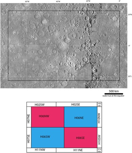
The main basemap used for the Kuiper geological map was the MDIS (Mercury Dual Imaging System) BDR (Basemap reduced Data Record) product (Table 1). BDRs are mosaics of WAC (wide-angle camera) and NAC (narrow-angle camera) images at the highest available spatial resolution (166 m/pixel). They include images with low emission angles at moderate to high incidence angles, which best highlight the topography. The images were received in several mosaics to have four tiles for each quadrangle (NE, SE, SW, NW). To map the Kuiper quadrangle, we considered a 5° of overlap with the surrounding quadrangles to allow a globally consistent interpretation of the geological units at the boundaries. Therefore, for the geological map, we used 14 tiles (Figure 1).

Figure 1. BDR mosaicked basemap of the Kuiper (H06) quadrangle in equirectangular projection with 5° overlap. Black square defines the boundary of the quadrangle. The mosaic includes 14 tiles: 4 for the Kuiper quadrangle and the remaining 10 for the adjacent quadrangles. Notes: Kuiper quadrangle BDR mosaicked basemap used for the mapping and a sketch indicating the mosaic's tales.

In addition to the BDRs, we used HIW and HIE Basemaps (Table 1), which include images with high incidence angle illuminated from the west and east, respectively. These helped us discern low relief topography (Figure 2(a, b)).

Figure 2. H06 supplementary basemaps. (a) 166 m/pixel HIE BDR MDIS mosaic; (b) 166 m/pixel HIW BDR MDIS mosaic; (c) 665 m/pixel enhanced color mosaic (Denevi et al., 2016); (d) 221.7 m/pixel DLR DTM mosaic (Preusker et al., 2017); (e) 332 m/pixel 3 color MDIS mosaic; (f) 665 m/pixel 8 color MDIS mosaic. Notes: Six tales showing the supplementary Kuiper quadrangle basemaps used for the mapping.

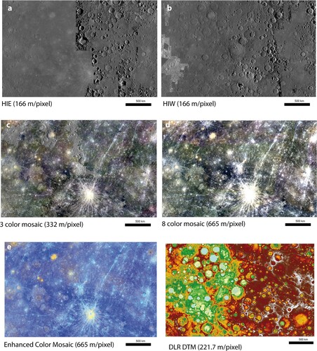
Coupled with the monochrome images, we used the MDIS WAC global color mosaic, with three and eight colors (Figure 2(c, d)) (Table 1). The spatial resolution of the mosaics, about 332 and 665 m/pixel for the three and eight colors, respectively, does not allow a detailed mapping, but they were useful to distinguish the boundaries of some geological units. Particularly suitable were the mosaics seen with R: 1000, G: 750, B: 430 nm. Also, the Enhanced color mosaic was used (Figure 2(e)), which, despite its moderate resolution (665 m/pixel), highlights the different color units well, and in particular, was useful to identify and map the volcanic deposits.

Table 1. Basemaps used for H06 geological mapping.

Original basemaps	Spatial resolution
MDIS_BDR_256PPD_Hxxdd^a	166 m/pixel
M1_M2_M3_M10Filt (Becker et al., 2009)	500 m/pixel
MDIS_v0_3color (MD3 basemap)	332 m/pixel
MDIS_v5_8color (MDR basemap)	665 m/pixel
MDIS_Basemap_Enhanced_color_mosaic	665 m/pixel
MDIS_HIE_256PPD_Hxxdd^a	166 m/pixel
MDIS_HIW_256PPD_Hxxdd^a	166 m/pixel
MSGR_DEM_DLR_EQ_H06_DM_222_I_v01	221 m/pixel

^a xx indicates the quadrangles and dd indicates the tiles NW, NE, SW, SE as shown in Figure 1.

The available basemaps based on MASCS (Mercury Atmospheric and Surface Composition Spectrometer) and XRS (X-ray spectrometer) data did not contribute significantly to the definition of the unit boundaries due to their lower resolution. For this reason, although some spectral studies have been carried out with those data on specific H06’s targets by other authors (e.g. D’Incecco et al., 2015; Weider et al., 2015), they have not been considered in this work.

2.2. Digital Terrain Model (DTM)

The main support for the analysis of the H06 topography came from the Deutsches Zentrum für Luft- und Raumfahrt (DLR) DTM (Figure 2(f)), built using stereo photogrammetry (Preusker et al., 2017) (Table 1). About 10.500 NAC and WAC MDIS stereo images, with an average resolution of 150 m/pixel, were collected to produce a final DTM with a spatial resolution of 221.7 m/pixel and vertical accuracy of about 30 m.

DTM was used to constrain the mapping and better to assess the stratigraphic relationship between the geological units.

3. Method

3.1. Projection and scale

To proceed with the mapping of H06 we firstly projected the basemaps. Because the Kuiper quadrangle is located in the equatorial area, we used an equirectangular projection. The reference datum for the projection was a sphere with a radius of 2440 km. For BDR images we projected each tile and then we mosaicked them to obtain the final BDR basemap. For projection and mosaicking, we used ISIS software.

The projected basemaps were then imported into the ArcGIS environment, which allows the geological features to be drawn as vector layers.

The output map scale is 1:3,000,000, which derives from a mapping scale with a two to five larger factors, following USGS guidelines (Tanaka et al., 2011). According to Galluzzi et al. (2016), five scale time larger mapping allows a cleaner and smoother linework; therefore, a map scale up to 1:600,000 can be used. However, considering the image resolution, the mapping scale (Sm) should be: $\mathrm{Sm}=\mathrm{Rr}\times 2000$where Rr is the raster resolution (Tobler, 1987). Since the BDR basemap is 166 m/pixel, the resulting mapping scale is 1:300,000. Hence, we mapped the Kuiper quadrangle at a scale ranging from 1:300,000 to 1:600,000.

3.2. Mapping method

To map the Kuiper quadrangle, we considered three main feature classes: (i) geological units, (ii) lineaments, and (iii) surface features. Following USGS guidelines (Tanaka et al., 2011), we classified the surface characterized by the same morphology/texture, albedo/color characteristic, and stratigraphic position as a geological unit. We indicated geological contacts between units in two ways: certain, where the contact is detected with confidence (the boundary between the units is clear and sharp); and approximate, where there is uncertainty in drawing the contact because the boundary between adjacent units is not well defined.

Lineaments include tectonic structures, crater rims, and pit rims. The tectonic structures are subdivided into (i) thrusts, including lobate scarps and high relief ridges (Watters & Nimmo, 2010); (ii) wrinkle ridges, appearing as a low relief arch with a narrow superposed ridge, localized mainly in smooth plains, considered to be formed by a combination of folding and thrust faulting (Watters et al., 2009); and (iii) general contractional faults, including all the reverse faults with no significant break nor a lobate trace, classified in this mode based on the observation of the dominant contractional nature of Mercury tectonics (e.g. Byrne et al., 2014). Normal faults have not been detected in the quadrangle.

Crater rims are mapped differently according to their diameter: for diameters equal to or higher than 20 km, craters are mapped with geological contacts defining the crater floor and crater material (i.e. crater walls, central peak and ejecta), whereas a continuous line with ornamental ticks, oriented inwards, defines their crests. For diameters between 5 and 20 km (small craters), only the crater crests are traced with a simple continuous line; no geological contacts are drawn to define their terrain. Finally, buried or degraded craters are mapped with a dashed line defining their crests.

Pit rims represent the edge of irregular pits that are interpreted to be volcanic vents.

Surface features include crater chains and clusters, hollows and faculae; these are diffuse bright red areas (Pegg et al., 2021; Wright et al., 2019) that have been considered as explosive volcanic deposits (Gillis-Davis et al., 2009; Goudge et al., 2014; Head et al., 2009; Jozwiak et al., 2018; Kerber et al., 2009, 2011; Murchie et al., 2008; Rothery et al., 2014; Thomas et al., 2014); . They have been mapped with polygons superposed on the geological units. Only features greater than 10 km (in length or width) were considered.

3.2.1. Crater classification

Previous geological maps classified craters into 5 classes (c1–c5), on the basis of their morphologies, assigning to each class a stratigraphic position (McCauley et al., 1981, recently reviewed by Kinczyk et al., 2016). However, using this classification, morphologically degraded craters often overly craters with a fresher aspect. To avoid this contradiction, following previous high-resolution maps (Galluzzi et al., 2016; Guzzetta et al., 2017; Mancinelli et al., 2016), we used a 3 classes classification. Other researchers (Pegg et al., 2021; Wright et al., 2019) chose to adopt 3 and 5 classes classification. In the 3 classes system, c1 and c3 are the end-members: c1 includes the oldest craters, characterized by a very degraded morphology, whereas c3 consists of the youngest craters, showing a fresh appearance. Finally, c2 includes the craters with intermediate morphologies between the two end-members. This classification avoids any conflict between relative ages implied by the crater degradation state and their relative stratigraphic ages.

4. Geological map description

The Kuiper quadrangle is mainly represented by crater material since several large craters and basins are found in the quadrangle. Some of them are very recent, and their ejecta blankets cover large areas. The second most extensive terrain in H06 is intercrater plains representing the oldest surface on Mercury. Smooth plains are limited and confined to some of the largest basin and crater floors.

4.1. Crater material

c3: craters with sharp, intact rims and well-preserved central peaks. The crater walls are extensively terraced. The floor appears rough or covered by smooth deposits, with a sharp contact between wall and floor. Ejecta can extend over 1 diameter from the crater rim, and be rayed and bright, with a hummocky surface texture (Figure 3(a, b)). The boundaries of distal ejecta are sharp. Numerous crater chains, radial to the crater rims, are often observed.

Figure 3. Crater classes of H06. (a) Kuiper crater as an example of c3 class; (b) 3-color image highlights the rayed ejecta of crater; (c) Brunelleschi crater as an example of c2 class. (d) Tchaikovsky crater as an example of c1 crater class (see text for more details about crater classification criteria). Notes: Four panels describing the different classes of craters mapped in the Kuiper quadrangle.

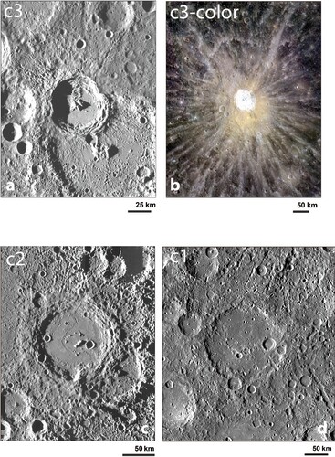
c2: craters with intermediate morphologies between c1 and c3. The rims are complete but not fresh. Terraces, if present, are not sharp. Ejecta are extensive, but distal ejecta lack clear boundaries (Figure 3(c)).

c1: degraded craters, with eroded, almost erased, rims. The crater floor of these craters shows a rough surface or it is covered by smooth deposits. Central peaks are absent or heavily eroded. Only the proximal ejecta are seldom detected. c1 craters are heavily affected by secondaries (Figure 3(d)).

Cfs: crater floor material, smooth. Planar floor affected by few craters, typical of craters c3 and c2. In c1 this feature may result from resurfacing. In c2 and c3 it could impact melt or lava flows.

Cfh: crater floor material, hummocky. Floor with a rough texture, moderately affected by craters. In c3 and c2 it represents mass wasting deposits coming from crater walls and emplaced on the floor, whereas in c1 it represents a degraded floor resulting from subsequent impacts.

4.2. Plains

Three different plains are recognized in H06: intercrater, intermediate, and smooth plains.

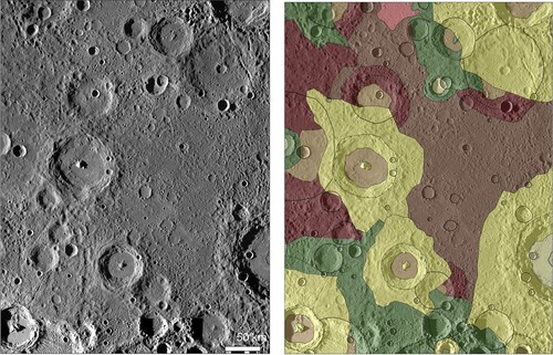
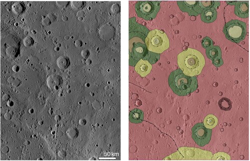
Intercrater plains (icp): they are the most extensive plains of H06 and Mercury in general. Heavily cratered terrains. The surface texture is rough and hummocky (Figure 4). In color images they do not have a peculiar color, showing from yellow to blue shades. Icp is the oldest surface present on the planet, with assigned Tolstojan to pre-Tolstojan age (> 3.9 Ga; Whitten et al., 2014). The origin of these plains is debated: they are commonly thought to represent effusive volcanic deposits although an impact origin cannot be excluded (Denevi et al., 2013; Whitten et al., 2014). They are superposed by craters belonging to all three classes (c1–c3).

Figure 4. Example area of intercrater plains in H06. This type of plain shows a rough texture and is heavily cratered. This leads to this terrain considering to be the oldest surface of Mercury. Basemap: 166 m/pixel BDR mosaic in equirectangular projection. Notes: An example of intercrater plains as shown in BDR mosaic and corresponding geological map of the same view.

Intermediate plains (imp): they are plains with intermediate characteristics between intercrater and smooth plain. Indeed, they are more cratered than the smooth plains but less than the intercrater ones (Figure 5). On H06, the boundaries of intermediate plains are not sharp and definable. Instead, a progressive transition with the intercrater plains is visible. In the transition area, the surface becomes progressively less cratered with crater rims progressively embayed by intermediate plains. Color maps do not help distinguish the boundary between intercrater and intermediate plains because they show a similar color to the surrounding plains. Some wrinkle ridges are observed, which helped us distinguish between intermediate and intercrater plains, because the latter have no wrinkle ridges. Imp are considered effusive volcanic deposits; however, their nature is not defined yet, and even the opportunity of mapping them as a distinct terrain is debated. Indeed, Imp were firstly detected and classified in the maps based on Mariner10 images, according to their morphological characteristics (e.g. Grolier & Boyce, 1984; Spudis & Prosser, 1984). Denevi et al. (2009), described them based on their spectral behaviour, which is different from smooth plains and low-reflectance material. Lately, Whitten et al. (2014) suggested that intermediate plains are composed of intercrater and smooth plains and consequently that they should be grouped into the latter units. In this work, we refer mainly to their morphological characteristics to distinguish the intermediate plains. This terrain is superposed only by c3 and c2 craters. Some c1 craters are detected, but they appear embayed or filled by the plains.

Figure 5. Example area of intermediate plains in H06. Intermediate plains show a less rough texture and are less cratered than intercrater plains. Basemap: 166 m/pixel BDR mosaic in equirectangular projection. Notes: An example of intermediate plain as shown in BDR mosaic and corresponding geological map of the same view.

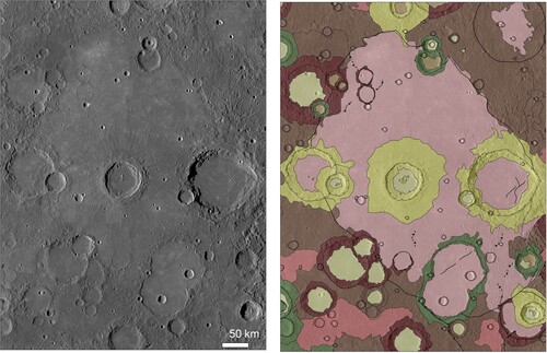
Smooth plains (sp): they are poorly cratered surfaces that show a smooth texture (Figure 6). In H06 smooth plains are not common and mainly localized into the larger basins. Frequently, wrinkle ridges are observed on the smooth plains. Smooth plains show distinctive color for the surrounding areas, which allows easy detection of the unit. The most extensive smooth plains of the quadrangle surround the Rudaki crater, and it has been classified by Denevi et al. (2013) as ‘intermediate reflectance plains’. The remaining smooth plains of H06 show a similar color, suggesting comparable reflectance characteristics. Smooth plains are thought to be recent effusive volcanic deposits (Denevi et al., 2013) with a Calorian age (3.7–3.9 Ga) (Denevi et al., 2013; Fassett et al., 2009; Head et al., 2011; Ostrach et al., 2011; Strom et al., 2008, 2011). They are superposed by c2 and c3 classes craters. Well-defined patches of smooth plains have also been detected in the proximal ejecta of some of the greater basins (i.e. Giotto, Lermontov, Handel basin), within their ejecta. These patches are interpreted as ponds of impact melt (Wright et al., 2019).

Figure 6. Example area of smooth plains in H06. This type of plain shows a smooth surface and is little affected by cratering. Basemap: 166 m/pixel BDR mosaic in equirectangular projection. Notes: An example of smooth plain as shown in BDR mosaic and corresponding geological map of the same view.

4.3. Units’ relative age

To establish the time relationship between the different units, we dated them through crater counting, following the method described in Crater Analysis Techniques Working Group (1979). We chose four sample areas: two intercrater, one intermediate and one smooth plain. For the latter two we chose the only extensive outcrops present on H06, for which a better statistic can be collected.

The obtained counts were arranged in cumulative size-frequency distribution (CSFD) and compared to each other to establish their relative ages (Figure 7(b)). Subsequently, the CSFDs were related with the Le Feuvre and Wiekzoreck Production Function (LWPF) to estimate their absolute model age (Figure 7(c–f)). The CSFD and the corresponding model ages confirm that icps are the oldest terrain in the quadrangle, with an age of 3.8 (±0.01) Ga (non-porous scaling law). This places the unit formation at the Late Heavy Bombardment (LHB) (Marchi et al., 2013).

Figure 7. Crater size-frequency distributions and age assessments for the four areas taken into account. (a) The location where crater counting was performed. Two intercrater plains (outlined in blue), one intermediate (outlined in green) and one smooth plain (outlined in pink) have been considered. (b) cumulative plot highlighting the relative ages of the different units. Intercrater plains (c–d), intermediate plains (e), and smooth plains (f) absolute ages obtained using the Le Feuvre and Wiekzoreck Production Function (LWPF) absolute model age. Notes: Series plots showing the crater-size frequency distributions resulting from the crater counting of different sample areas for intercrater, intermediate and smooth plains.

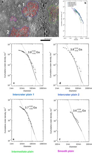
The intermediate plains’ age stands between smooth and intercrater, with a value of 3.7 (±0.02) Ga (non-porous scaling law). An overlap with intercrater plain CSFDs is observed for craters smaller than 20 km, which is probably due to the presence of secondaries, which in this range of diameter could influence the statistics. For intercrater and intermediate plains, the non-porous scaling law has been chosen since only craters larger than 20 km were considered as the best fit with LWPF. Therefore, hard rock terrain is involved.

The smooth plains are the youngest geological unit, with an age of 3.6 (+0.04–0.01) Ga, based on a porous scaling law. We used this scaling law due to the modest dimension of craters that affected only the upper surface, which is likely fractured by subsequent impacts and lava flows cooling (Giacomini et al., 2020; Schultz, 1993).

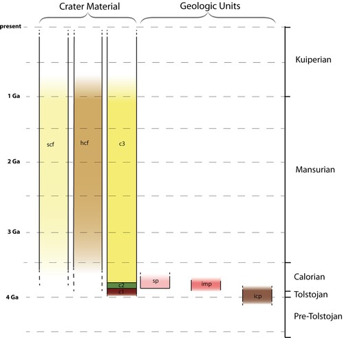
On the basis of the observed superposition relationships among the different units and the absolute model ages obtained in this work, and from the estimations of previous authors (Byrne et al., 2016; Marchi et al., 2013; Neukum et al., 2001; Ostrach et al., 2015; Whitten et al., 2014), we propose the stratigraphic scheme shown in Figure 8.

Figure 8. Schematic correlation of H06 map units based on superposition relations and the estimated ages of SP, IMP and ICP from the literature (Byrne et al., 2016; Marchi et al., 2013; Neukum et al., 2001; Ostrach et al., 2015; Whitten et al., 2014). Basal ages for the chrono-stratigraphic systems are from Spudis and Guest (1988). In this scheme, no spectral units have been taken into account. For a correlation among geological units, MDIS color units, and MASCS units see D’Incecco et al., 2015. Notes: Diagram showing the time-relationship between the different units mapped in Kuiper quadrangle.

5. Conclusion

We compiled a geological map of the Kuiper quadrangle (H06) using MESSENGER data at a scale of 1:3M. The available dataset has allowed building a more detailed map than the previous 1:5M map of the quadrangle (De Hon et al., 1981), based on Mariner10 images. The criteria used for the mapping follow previous quadrangle geological maps (Galluzzi et al., 2016; Guzzetta et al., 2017; Mancinelli et al., 2016; Wright et al., 2019).

We mapped geological units, lineaments and surface features. The mapped geological units were grouped into crater material, belonging to three classes (c1–c3) based on degradation degree, and plains (smooth, intermediate and intercrater plains). Lineaments were distinguished in crater rims and structures. Finally, surface features include crater chains, hollows and pyroclastic materials.

The crater counting performed on the geological units confirms the classification of IMP as a distinct unit, distinguishable morphologically and stratigraphically from smooth plains, following Galluzzi et al. (2016). This map is part of a wider project devoted to the global mapping of the Mercury surface (Galluzzi et al., 2021).

Software

To produce our map we used ESRI ArcGIS software. Some images have been processed using ISIS3 (Integrated Software for Imagers and Spectrometers v3) software (Eliason, 1997; Gaddis et al., 1997; Torson & Becker, 1997), developed by the USGS (United States Geological Survey). To perform the crater counting we used Crater Tools (Kneissl et al., 2011), whereas to plot the results of the counts, we used the Craterstats2 (e.g. see Michael & Neukum, 2010).

Acknowledgments

We thank D.A. Rothery, H. Apps, and P. D’Incecco, who provided detailed and helpful suggestions that improved the quality of the manuscript and map. The authors acknowledge the use of MESSENGER data processed by NASA/Johns Hopkins University Applied Physics Laboratory/Carnegie Institution of Washington.

Disclosure statement

No potential conflict of interest was reported by the author(s).

Data availability statement

The data and materials that support the results of this work are freely available upon reasonable request.

Additional information

Funding

Part of this work was funding from the Italian Space Agency (ASI) under ASI-INAF agreement 2017-47-H.0.

References

- Banks, M. E., Xiao, Z., Braden, S. E., Barlow, N. G., Chapman, C. R., Fassett, C. I., & Marchi, S. (2017). Revised constraints on absolute age limits for Mercury's Kuiperian and Mansurian stratigraphic systems. Journal of Geophysical Research: Planets, 122(5), 1010–1020. https://doi.org/10.1002/2016JE005254
- Becker, K. J., Robinson, M. S., Becker, T. L., Weller, L. A., Turner, S., Nguyen, L., Selby, C., Denevi, B. W., Murchie, S. L., McNutt, R. L., & Solomon, S. C. (2009, December 14-18). Near global mosaic of mercury. AGU. Fall meeting 2009, abstract #P21A-1189.
- Byrne, P. K., Klimczak, C., Celâl Şengör, A. M., Solomon, S. C., Watters, T. R., & Hauck, S. A. (2014). Mercury’s global contraction much greater than earlier estimates. Nature Geoscience, 7(4), 301–307. https://doi.org/10.1038/ngeo2097
- Byrne, P. K., Ostrach, L. R., Fassett, C. I., Chapman, C. R., Denevi, B. W., Evans, A. J., & Solomon, S. C. (2016). Widespread effusive volcanism on Mercury likely ended by about 3.5 Ga. Geophysical Research Letters, 43(14), 7408–7416. https://doi.org/10.1002/2016GL069412
- De Hon, R. A., Scott, D. H., & Underwood, J. R. (1981). Geologic map of the Kuiper (h-6) quadrangle of Mercury. USGS Geological Survey. Map I, 1233.
- Denevi, B. W., Ernst, C. M., Meyer, H. M., Robinson, M. S., Murchie, S. L., Whitten, J. L., & Peplowski, P. N. (2013). The distribution and origin of smooth plains on Mercury. Journal of Geophysical Research: Planets, 118(5), 891–907. https://doi.org/10.1002/jgre.20075
- Denevi, B. W., Ernst, C. M., Prockter, L. M., Robinson, M. S., Spudis, P. D., Klima, R. L., & Kinczyk, M. J. (2016). The origin of Mercury’s oldest surfaces and the nature of intercrater plains resurfacing. In Lunar and Planetary Science Conference, 47th, #1624, bibcode: 2016LPI … 47.1624D.
- Denevi, B. W., Robinson, M. S., Solomon, S. C., Murchie, S. L., Blewett, D. T., & Domingue, D. L., … Chabot, N. L. (2009). The evolution of Mercury's crust: A global perspective from MESSENGER. Science, 324(5927), 616–618. https://doi.org/10.1126/science.1172226
- D’Incecco, P., Helbert, J., D’Amore, M., Maturilli, A., Head, J. W., Klima, R. L., Izenberg, N. R., McClintock, W. E., Hiesinger, H., & Ferrari, S. (2015). Shallow crustal composition of Mercury as revealed by spectral properties and geological units of two impact craters. Planet. Space Sci, 119, 250–263. https://doi.org/10.1016/j.pss.2015.10.007
- Eliason, E. M. (1997, March 17-21). Production of digital image modelsusing the ISIS system. In 28th Annual Lunar and Planetary Science Conference. Houston, TX.
- Fassett, C. I., Head, J. W., Blewett, D. T., Chapman, C. R., Dickson, J. L., Murchie, S. L., & Watters, T. R. (2009). Caloris impact basin: Exterior geomorphology, stratigraphy, morphometry, radial sculpture, and smooth plains deposits. Earth and Planetary Science Letters, 285(3), 297–308. https://doi.org/10.1016/j.epsl.2009.05.022
- Gaddis, L., Anderson, J., Becker, K., Becker, T., Cook, D., Edwards, K., Eliason, E., Hare, T., Kieffer, H., Lee, E. M., Mathews, J., Soderblom, L., Sucharski, T., Torson, J., Mcewen, A. (1997, March 17-21). An overview of the integrated software for imaging spectrometers (ISIS). 28th Annual Lunar and Planetary Science Conference. Houston, TX.
- Galluzzi, V., Guzzetta, L., Ferranti, F., Di Achille, G., Rothery, D. A., & Palumbo, P. (2016). Geology of the Victoria quadrangle (H02), Mercury. Journal of Maps, 12(Suppl 1), 227–238. https://doi.org/10.1080/17445647.2016.1193777
- Galluzzi, V., Rothery, D. A., Giacomini, L., Guzzetta, L., El Yazidi, M., Ferranti, L., Lennox, A. R., Malliband, C., Man, B., Massironi, M., Palumbo, P., Pegg, D. L., Tognon, G., & Wright, J. (2021). European quadrangle mapping of Mercury: Status report. Planetary Geologic Mappers 2021, (LPI Contrib. No. 2610), p. 7027.
- Giacomini, L., Massironi, M., Galluzzi, V., Ferrari, S., & Palumbo, P. (2020). How old are the Mercury’s thrust systems? New clues on the thermal evolution of the planet. Geoscience Frontiers, 11(3), 855–870. https://doi.org/10.1016/j.gsf.2019.09.005
- Gillis-Davis, J. J., Blewett, D. T., Gaskell, R. W., Denevi, B. W., Robinson, M. S., Strom, R. G., Solomon, S. C., & Sprague, A. L. (2009). Pit-floor craters on Mercury: Evidence of near-surface igneous activity. Earth and Planetary Science Letters, 285(3-4), 243–250. https://doi.org/10.1016/j.epsl.2009.05.023
- Goudge, T. A., Head, J. W., Kerber, L., Blewett, D. T., Denevi, B. W., Domingue, D. L., Gillis-Davis, J. J., Gwinner, K., Helbert, J., Holsclaw, G. M., Izenberg, N. R., Klima, R. L., McClintock, W. E., Murchie, S. L., Neumann, G. A., Smith, D. E., Strom, R. G., Xiao, Z., Zuber, M. T., & Solomon, S. C. (2014). Global inventory and characterisation of pyroclastic deposits on Mercury: New insights into pyroclastic activity from MESSENGER orbital data. Journal of Geophysical Research: Planets, 119(3), 635–658. https://doi.org/10.1002/2013JE004480
- Grolier, M. J., & Boyce, J. M. (1984). Geologic map of the Borealis region (H-1) of Mercury. USGS Misc. Investig. Ser. Map I–, 1660.
- Guzzetta, L., Galluzzi, V., Ferranti, L., & Palumbo, P. (2017). Geology of the Shakespeare quadrangle (H03), Mercury. Journal of Maps, 13(2), 227–238. https://doi.org/10.1080/17445647.2017.1290556
- Guzzetta, L., Lewang, A., Hiesinger, H., Ferranti, L., & Palumbo, P. (2021). Geologic map of the Beethoven Quadrangle (H07), Mercury. SGI2021, abstract.
- Hapke, B., Danielson, G. E., Klaasen, K., & Wilson, L. (1975). Photometric observations of Mercury from Mariner 10. Journal of Geophysical Research, 80(17), 2431–2443. https://doi.org/10.1029/JB080i017p02431
- Head, J. W., Chapman, C. R., Strom, R. G., Fassett, C. I., Denevi, B. W., Blewett, D. T., & Nittler, L. R. (2011). Flood volcanism in the northern high latitudes of Mercury revealed by MESSENGER. Science, 333(6051), 1853–1856. https://doi.org/10.1126/science.1211997
- Head, J. W., Murchie, S. L., Prockter, L. M., Solomon, S. C., Chapman, C. R., Strom, R. G., Watters, T. R., Blewett, D. T., Gillis-Davis, J. J., Fassett, C. I., Dickson, J. L., Morgan, G. A., & Kerber, L. (2009). Volcanism on mercury: Evidence from the first MESSENGER flyby for extrusive and explosive activity and the volcanic origin of plains. Earth and Planetary Science Letters, 285(3-4), 227–242. https://doi.org/10.1016/j.epsl.2009.03.007
- Jozwiak, L. M., Head, J. W., & Wilson, L. (2018). Explosive volcanism on Mercury: Analysis of vent and deposit morphology and modes of eruption. Icarus, 302, 191–212. https://doi.org/10.1016/j.icarus.2017.11.011
- Kerber, L., Head, J. W., Blewett, D. T., Solomon, S. C., Wilson, L., Murchie, S. L., Robinson, M. S., Denevi, B. W., & Domingue, D. L. (2011). The global distribution of pyroclastic deposits on Mercury: The view from MESSENGER flybys 1-3. Planetary and Space Science, 59(15), 1895–1909. https://doi.org/10.1016/j.pss.2011.03.020
- Kerber, L., Head, J. W., Solomon, S. C., Murchie, S. L., Blewett, D. T., & Wilson, L. (2009). Explosive volcanic eruptions on Mercury: Eruption conditions, magma volatile content, and implications for interior volatile abundances. Earth and Planetary Science Letters, 285(3-4), 263–271. https://doi.org/10.1016/j.epsl.2009.04.037
- Kinczyk, M. J., Prockter, L. M., Chapman, C. R., & Susorney, H. C. M. (2016, March 21-25). A morphological evaluation of crater degradation on mercury: Revisiting crater classification using MESSENGER data. Lunar Planetary Science Conference, 47th, #1573, bibcode: 2016LPI … 47.1573 K.
- Kneissl, T., Van Gasselt, S., & Neukum, G. (2011). Map-projection-independent crater size-frequency determination in GIS environments - New software tool for ArcGIS. Planetary and Space Science, 59(11), 1243–1254. https://doi.org/10.1016/j.pss.2010.03.015
- Le Feuvre, M., & Wieczorek, M. A. (2011). Nonuniform cratering of the moon and a revised crater chronology of the inner Solar System. Icarus, 214(1), 1–20. https://doi.org/10.1016/j.icarus.2011.03.010
- Malliband, C. C., Rothery, D. A., Balme, M. R., & Conway, S. J. (2018). 1:3M geological mapping of the Derain (H-10) quadrangle of Mercury. Mercury: Current and Future Science, 2018, abstract #2047.
- Mancinelli, P., Minelli, F., Pauselli, C., & Federico, C. (2016). Geology of the raditladi quadrangle, Mercury (H04). Journal of Maps, 5647, 1–13. https://doi.org/10.1080/17445647.2016.1191384
- Marchi, S., Chapman, C. R., Fassett, C. I., Head, J. W., Bottke, W. F., & Strom, R. G. (2013). Global resurfacing of Mercury 4.0–4.1 billion years ago by heavy bombardment and volcanism. Nature, 499(7456), 59–61. https://doi.org/10.1038/nature12280
- McCauley, J. F., Guest, J. E., Schaber, G. G., Trask, N. J., & Greeley, R. (1981). Stratigraphy of the Caloris basin, Mercury. Icarus, 47(2), 184–202. https://doi.org/10.1016/0019-1035(81)90166-4
- Michael, G. G., & Neukum, G. (2010). Planetary surface dating from crater size-frequency distribution measurements: Partial resurfacing events and statistical age uncertainty. Earth and Planetary Science Letters, 294(3), 223–229. https://doi.org/10.1016/j.epsl.2009.12.041
- Murchie, S. L., Watters, T. R., Robinson, M. S., Head, J. W., Strom, R. G., Chapman, C. R., Solomon, S. C., Mcclintock, W. E., Prockter, L. M., Domingue, D. L., & Blewett, D. T. (2008). Geology of the Caloris basin, Mercury: A view from MESSENGER. Science, 321(5885), 73–76. https://doi.org/10.1126/science.1159261
- Neukum, G., Oberst, J., Hoffmann, H., Wagner, R., & Ivanov, B. A. (2001). Geologic evolution and cratering history of Mercury. Planetary and Space Science, 49(14-15), 1507–1521. https://doi.org/10.1016/S0032-0633(01)00089-7
- Ostrach, L. R., Robinson, M. S., Denevi, B. W., & Thomas, P. C. (2011, March 7-11). Effects of incidence angle on crater counting observations. In Lunar and Planetary Science conference. 42nd, #1202, bibcode: 2011LPI … 42.1202O.
- Ostrach, L. R., Robinson, M. S., Whitten, J. L., Fassett, C. I., Strom, R. G., Head, J. W., & Solomon, S. C. (2015). Extent, age, and resurfacing history of the northern smooth plains on Mercury from MESSENGER observations. Icarus, 250, 602–622. https://doi.org/10.1016/j.icarus.2014.11.010
- Pegg, D. L., Rothery, D. A., Balme, M. R., Conway, S. J., Malliband, C. C., & Man, B. (2021). Geology of the Debussy quadrangle (H14), Mercury. Journal of Maps, 17(2), 859–870. https://doi.org/10.1080/17445647.2021.1996478
- Preusker, F., Stark, A., Oberst, J., Matz, K.-D., Gwinner, K., & Watters, T. R. (2017). Toward high-resolution global topography of Mercury from MESSENGER orbital stereo imaging: A prototype model for the H6 (Kuiper) quadrangle. Planetary and Space Sci, 142, 26–37. https://doi.org/10.1016/j.pss.2017.04.012
- Rothery, D. A., Thomas, R. J., & Kerber, L. (2014). Prolonged eruptive history of a compound volcano on Mercury: Volcanic and tectonic implications. Earth and Planetary Science Letters, 385, 59–67. https://doi.org/10.1016/j.epsl.2013.10.023
- Schultz, R. A. (1993). Brittle strength of basaltic rock masses with applications to Venus. Journal of Geophysical Research, 98(E6), 10883–10895. https://doi.org/10.1029/93JE00691
- Spudis, P. D., & Guest, J. E. (1988). Stratigraphy and geologic history of Mercury. In F. Vilas, C. R. Chapman, & M. S. Matthews (Eds.), Mercury (pp. 118–164). University of Arizona Press. ISBN: 0816510857.
- Spudis, P. D., & Prosser, J. G. (1984). Geologic map of the Michaelangelo (H-12) Quadrangle of Mercury, I-1659. USGS, Reston, VA.
- Strom, R. G., Banks, M. E., Chapman, C. R., Fassett, C. I., Forde, J. A., Head, J. W., & Solomon, S. C. (2011). Mercury crater statistics from MESSENGER flybys: Implications for stratigraphy and resurfacing history. Planetary and Space Science, 59(15), 1960–1967. https://doi.org/10.1016/j.pss.2011.03.018
- Strom, R. G., Chapman, C. R., Merline, W. J., Solomon, S. C., & Head, J. W. (2008). Mercury cratering record viewed from MESSENGER’s first flyby. Science, 321(5885), 79–81. https://doi.org/10.1126/science.1159317
- Strom, R. G., & Sprague, A. L. (2003). Exploring Mercury. Springer Praxis. ISBN: 9781852337315.
- Tanaka, K. L., SkinnerJr.J. A., & Hare, T. M. (2011). Planetary geologic mappers handbook. USGS Astrogeology Science Center. Retrieved fromhttp://astrogeology.usgs.gov/search/details/Docs/Mappers/PGM_Handbook_2011/pdf
- Thomas, R. J., Rothery, D. A., Conway, S. J., & Anand, M. (2014). Mechanisms of explosive volcanism on Mercury: Implications from its global distribution and morphology. Journal of Geophysical Research: Planets, 119(10), 2239–2254. https://doi.org/10.1002/2014JE004692
- Tobler, W. (1987). Measuring spatial resolution. Proceedings of the Land Resources Information Systems Conference, Beijing, pp. 12–16.
- Torson, J. M., & Becker, K. J. (1997, March 17-21). ISIS – A software architecture for processing planetary images. 28th Annual Lunar and Planetary Science Conference. Houston, TX.
- Watters, T. R., & Nimmo, F. (2010). Tectonism on Mercury. In R. A. Schultz, & T. R. Watters (Eds.), Planetary tectonics (pp. 15–80). Cambridge Univ Press.
- Watters, T. R., Solomon, S. C., Robinson, M. S., Head, J. W., André, S. L., Hauck IIS. A., & Murchie, S. L. (2009). The tectonics of Mercury: The view after MESSENGER’s first flyby. Earth and Planetary Science Letters, 285(3-4), 283–296. https://doi.org/10.1016/j.epsl.2009.01.025
- Weider, S. Z., Nittler, L. R., Starr, R. D., Crapster-Pregont, E. J., Peplowski, P. N., Denevi, B. W., Head, J. W., Byrne, P. K., Hauck II, S. A., Ebel, D. S., & Solomon, S. C. (2015). Evidence for geochemical terranes on Mercury: Global mapping of major elements with MESSENGER's X-ray spectrometer. Earth and Planetary Science Letters, 416, 109–120. https://doi.org/10.1016/j.epsl.2015.01.023
- Whitten, J. L., Head, J. W., Denevi, B. W., & Solomon, S. C. (2014). Intercrater plains on Mercury: Insights into unit definition, characterization, and origin from MESSENGER datasets. Icarus, 241, 97–113. https://doi.org/10.1016/j.icarus.2014.06.013
- Wright, J., Rothery, D. A., Balme, M. R., & Conway, S. J. (2019). Geology of the Hokusai quadrangle (H05), Mercury. Journal of Maps, 15(2), 509–520. https://doi.org/10.1080/17445647.2019.1625821