Geomorphological slope units of the Himalayas

ABSTRACT

Slope units represent surface slopes by means of polygons delimited by drainage and divide lines obtained on a digital topography. Objective slope unit delineation for a given digital elevation model is still an open issue and, often, a limitation that may dictate the use of a more traditional pixel-based approach for spatial analysis. Availability of slope unit maps facilitates many kinds of studies and allows scholars to focus on specific scientific issues rather than on preparing sound mapping units from scratch for their research. Here, we present a slope unit map of a large portion of the Himalayas. The map is prepared following a widely tested, parameter-free optimization algorithm. The area encompassed by the map is relevant to studies of the well-known 2015 Gorkha earthquake and monsoons, which makes it relevant to a vast portion of the scientific community working in natural hazards including, but not limited to, landslide scientists and practitioners. The map contains 112,674 polygons with average area of 0.38 km${}^2$ and is published in vector form. The map is accompanied by a selection of data including morphometric and thematic quantities. In addition to describing the rationale behind the delineation of the polygonal map and selected data, we describe an application devoted to unsupervised terrain classification. We applied a k-means clustering procedure with two strategies: one at (coarser) basin scale and one at (finer) slope unit scale. We show similarities and differences between the two classification strategies, highlighting the role of the slope unit subdivision in the two cases.

KEYWORDS:

• Geomorphometry
• Gorkha
• mapping units
• terrain classification
• natural hazards
• automatic delineation

1. Introduction

Slope units (SU) are becoming a popular choice as mapping units for a variety of studies, mostly related to natural hazards. Although SU were proposed long ago as an alternative to pixel-based approaches, it took a long time for them to be considered as an effective tool. Recently, automated tools and objective delineation criteria made it possible to efficiently obtain SU maps in large areas, independently on any data beyond a digital elevation model (DEM). Moreover, well-defined optimization criteria allow for overcoming common pitfalls in SU delineation, mostly related to subjectivity and to narrow-scope requirements of specific applications.

Reliable SU maps are an effective tool for a few reasons. First and foremost, a pre-delineated map is readily available for scientists, practitioners and possibly decision makers with a professional interest in the area. They may focus on applications of the map for their particular purpose, instead of spending time to delineate mapping units. Second, adoption of a common map, either at different times by the same working group or by different working groups, provides a baseline for comparison and/or update of existing models and results.

In this paper, we focused on a large part of the Himalayas, mostly overlapping Central Nepal and a small part of China. The area covers about 43,000 km${}^2$ and is of great interest for it is a seismically active area, also subject to monsoons and extensive landslide phenomena. The area has average population density of about 178 people/km${}^2$, with larger density in the Southern lower-elevation belts. Most of the study area was affected by the 2015 Gorkha earthquake, which killed more than 9,000 people, damaged over 600,000 structures and triggered over 20,000 landslides (Gnyawali & Adhikari 2017; Kargel et al. 2016; Roback et al. 2018, 2017; Zhang et al. 2016). Thus it is of vast scientific interest and the subject of many publications (Cook et al. 2018; Marc et al. 2019; Pokharel et al. 2021).

We describe an optimized SU map containing 112,674 polygons of various shapes and sizes. We obtained the map using the software and methods of Alvioli et al. (2020, 2016). Slope units produced with the same method were used before for landslide studies by some of us (Alvioli et al. 2018, 2021; Bornaetxea et al. 2018; Doménech et al. 2020; Jacobs et al. 2020; López-Vinielles et al. 2021; Schlögel et al. 2018; Tanyaş, Rossi, et al. 2019; Tanyaş, van Westen, et al. 2019) and other scholars as well (Amato et al. 2020; Camilo et al. 2017; Li & Lan 2020). Different delineation methods exist; the most simplistic ones are based on DEM inversion technique, while others rely on different morphometric considerations, e.g. Chen et al. (2020). We publish the map in vector format, with an attribute table including the values of data variables as well as morphometric and thematic quantities for each row, i.e. for each SU polygon.

Eventually, as an application of the map, we propose a terrain classification of the area (i.e. subdivision into a given number of sub-areas using geomorphological considerations) considering either (larger) basins, or (much smaller) individual SU, as aggregation domains. A similar effort was proposed by Alvioli et al. (2020) in the case of Italy, at basin level. The classification at SU level, performed aggregating morphometric variables within each SU, is novel to this work as it was obtained using different sets of classification variables fed to the k-means clustering algorithm.

This work is organized as follows. Section 2 describes the data used in this work. Section 3 describes SU delineation (main goal) and terrain classification (an application of the map). Results are shown in Section 4; in Section 5, results are discussed and conclusions are drawn. Section 6 describes the published digital map and attribute table, along with download link; Section 7 lists software used here; Section 9 gives geolocation information. Appendix 1 (supplement) described alternative terrain classifications, for the interested reader. Appendix 2 describes the published printable map (supplement).

2. Materials

We implemented an automatic procedure to delineate slope units based on the software r.slopeunits (Alvioli et al. 2016) and an upgraded optimization strategy, introducing an improved way to get rid of very local effects. The procedure uses Shuttle radar topography mission (SRTM) elevation data at 30-m resolution, selecting the data tiles overlapping with a polygonal area of interest. Figure 1(a) shows the location of the study area (filled purple contour).

Figure 1. The study area, about 43,000 km${}^2$ mostly in Nepal and with a small portion in China. (a) The background is a shaded relief of terrain, overlain to the Cartosat DEM and colorized with the typical elevation color ramp; the study area is the purple contour. (b) The extent of the 15 SRTM DEM tiles used for this work; black lines: hydrological basins used as local domains of the procedure for SU delineation (Alvioli et al. 2020, 2016). Purple filled polygons: basins corresponding to the study area. Yellow and green filled polygons: first- and second-order basins, respectively, ranked by proximity to the most peripheral purple ones. All maps in EPSG:32645.

Subdivision in hydrological basins of the Gorkha area, in Himalaya.

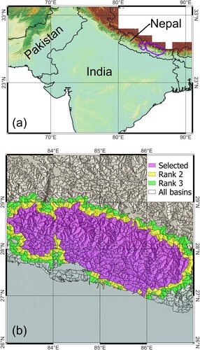
We selected 15 SRTM tiles,¹ whose spatial extent is shown in Figure 1(b). SRTM elevation data was only used to run the r.slopeunit software in a parametric way. In fact, the software depends on a few parameters, and the values of the most relevant parameters must be selected, i.e. optimized, in a sound way. The first step of the optimization procedure is to draw hydrological basins, shown in Figure 1(b) as polygons of different colors; purple polygons represent the area of interest. Next, we used Cartosat elevation data obtained specifically for the Indian sub-continent, to perform further morphometric analysis within slope units (https://bhuvan.nrsc.gov.in).

None other than the above-mentioned data was used for this work, as delineation and optimization of slope units only rely on the digital topography. The same is true for the subsequent terrain classification with k-means clustering. Ancillary data was used, however, to populate the attribute table associated with the map published here. Namely, we added geological information (Hartmann & Moosdorf 2012), presence of landslides induced by the Gorkha Earthquake of 2015 (Pokharel et al. 2021; Roback et al. 2017), and mean daily and annual precipitation (Funk et al. 2015).

3. Methods

We have run the r.slopeunits, a specialized code for automatic and parametric delineation of slope units (Alvioli et al. 2016). We further optimized input parameters of the code using the aspect segmentation metric, first introduced by Espindola et al. (2006) and adapted to optimize SU delineation (Alvioli et al. 2020).

We first obtained hydrological basins for the whole area within the selected SRTM tiles, ending up with 1,436 basins with an average area of 92.2 km${}^2$, shown as black polygons, either filled with colors or transparent, in Figure 1(b). The transparent basins were not used in the remaining of this work; the actual basins of interest, here, are in purple (450 basins); yellow polygons are the first-adjacent basins, and green polygons the second-adjacent. Ranking of the basins based on proximity is useful for the optimization of the software's input parameters, as described below.

3.1. Optimized slope unit delineation

The software r.slopeunits is an adaptive tool, in that it delineates SU polygons of different shapes and sizes according to the local surface roughness. It is a parametric software, because it uses a few key parameters that need tuning, in specific areas, to obtain the best result. The most relevant input parameters are called minimum area, $a_{min}$, a tentative minimum area for output polygons, and minimum circular variance, $c_{min}$, representing a measure of homogeneity of each polygon in terms of slope aspect.

The optimization procedure for the input parameters of the r.slopeunits software was described in detail in Alvioli et al. (2020); here, we slightly modified such procedure to remove somewhat arbitrary steps. The following steps summarize the essentials of the optimization method:

Optimization of slope units: convergence of numerical parameters.

Figure 2. The series of optimal parameters $a_{min}$ (a) and $c_{min}$ (b) for domains of increasing size with increasing rank, up to rank 3 (cf. Section 3.1). Each curve in the two boxes represents one of the 450 purple basins in Figure 1, for a random subset of 30 basins. Horizontal error bars represent the range of distances existing between any two points within the spatial domain under consideration. For each curve, the limit for large distances represents the optimal value of the parameter.

(1)	Run r.slopeunits with a pre-defined set of parameter combinations, in each basin. For each of the colored basins in Figure 1, which cover the actual area of interest, we run the r.slopeunits software for 49 different combinations of the ($a_{min}$, $c_{min}$) input parameters. This is a grid of combinations with $a_{min}$ varying in (50 k, 100 k, 150 k, 200 k, 250 k, 250 k, 300 k, 400 k) m${}^2$ and $c_{min}$ varying in (0.01, 0.1, 0.15, 0.2, 0.3, 0.4, 0.5). This resulted in 49 different sets of SU for each of the 658 colored (either in purple, yellow or green) basins in Figure 1; in fact, the optimization procedure involves a larger number of basins than those of actual interest (in purple), because it requires nearest- (in yellow) and second-nearest (in green) neighboring basins. The requirement of considering neighboring basins to optimize parameters in each specific basin stems from avoiding SU delineation to be overly specific on very local features and to obtain a smooth transition across borders of adjacent basins.
(2)	Calculate aspect segmentation function $F(a_{min},c_{min})$ for each combination (i.e. in each SU set). For each of the 450 purple basins of Figure 1, and for each set of SU in the basin, we calculated the aspect segmentation function F($a_{min}$, $c_{min}$). The function F($a_{min}$, $c_{min}$) is our measure of how well each slope unit map (i.e. each ($a_{min}$, $c_{min}$) combination) splits the topography into well-defined areas, in terms of terrain aspect. Maximization of F($a_{min}$, $c_{min}$) in each basin of interest provides the rank-1 optimal combination ($a_{opt}^{(1)}$, $c_{opt}^{(1)}$), for that specific basin. Thus, after this step, each basin is associated with a parameter combination which locally optimizes SU delineation.
(3)	Maximize $F(a_{min},c_{min})$ within different spatial domains, of increasing size. The optimized values in each basin can be spatially correlated with those in adjacent basins. For this reason, we seek for convergence of values optimized over spatial domains of increasing size. To this end, for each of the purple basins we calculated the function F($a_{min}$, $c_{min}$) for SU sets delineated in the area encompassed by of all the neighboring basins. Maximization of such function provides rank-2 optimized values of the parameters, ($a_{opt}^{(2)}$, $c_{opt}^{(2)}$). Iterating the procedure of spatial domain expansion, calculation of F($a_{min}$, $c_{min}$) in the newly selected (larger, at each iteration) area, and maximization of the function F in that area, we obtained rank-n optimized parameters: ($a_{opt}^{(n)}$, $c_{opt}^{(n)}$), with n = 2, 3. Figure 2 shows the series of the parameters $a_{min}$ and $c_{min}$ (for a random subset of 30 basins out of the total 450, for illustration purposes) up to rank-3 basins. Optimized values at each rank are plotted as a function of the average distance of any two points within the spatial domain considered in the calculation; a horizontal bar describes the distribution of distances, for each calculated point.
(4)	Fit of the series of optimal values obtained from maximization in the different domains. We modified the optimization procedure of Alvioli et al. (2020) in two ways. First, we calculated optimized values ($a_{opt}^{(n)}$, $c_{opt}^{(n)}$) within all of the basins at rank-n at the same time, instead of considering all of the possible n-tuple of basins; this reduced the computing time without loss of accuracy. Second, we weighted each point in Figure 2 with a distribution of distances from the centroid of the basin of interest (denoted here as rank-1 basin). This is an improvement on the method of Alvioli et al. (2020), in that the previous series was weighted with an (arbitrary) inverse-rank criterion. The distribution of distances is obtained calculating the distance of any point within the rank-n aggregation domain from the centroid of the basin of interest.
(5)	Extract the limiting values of each series (for each basin) and delineate the final SU map. Optimized values $a_{opt}$ and $c_{opt}$ are the limits of the corresponding series ($a_{opt}^{(1)}$, $a_{opt}^{(2)}$, $a_{opt}^{(3)}$). Fit of the series (taking into account horizontal error bars using the ‘xerror’ option in the Gnuplot software, http://www.gnuplot.info/) for individual basins, with a function $y(x)=A+B/x$, provide the limiting value, A, where the series is strictly monotonic; we used a simple average, otherwise. A few examples of strictly decreasing, constant, and strictly increasing series are shown in Figure 2. We performed the fit for both parameters $a_{min}$ and $c_{min}$. The limiting values of each series, if monotonic, and the simple average, for non-monotonic series, are the values used for initializing the parameters $a_{min}$ and $c_{min}$ in r.slopeunits, for a final (single) run of the software, for each of the basins of interest. The collection of the resulting SU maps in each basin of interest (purple polygons in Figure 1) is the final map and the main result of this work.

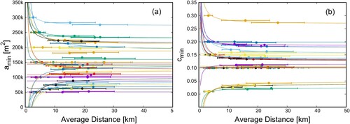The final SU map is published as a vector layer. We furnished the published digital map with a database of morphometric and thematic variables, to make it more useful and easy to use by third parties.

Morphometric variables include: elevation, slope, relief (elevation range), planar and tangential curvature, topographic wetness index (TWI) and vector ruggedness index (VRM); for each such variable, we inserted in the database a column listing the mean value and standard deviation of the variable (calculated within each slope unit). Additional morphometric information is the percentage presence of landforms defined by the geomorphons model (Jasiewicz & Stepinski 2013). We found that the five most common such landforms are ridge, spur, slope, hollow, and valley; presence of other landforms is negligible (Pokharel et al. 2021).

Thematic variables include a flag denoting presence of earthquake induced landslides, from the 2015 Gorkha earthquake event (Pokharel et al. 2020, 2021). We considered the three larger landslide inventories prepared by three different groups, namely Zhang et al. (2016), Gnyawali and Adhikari (2017) and Roback et al. (2017). Thematic variables also included geology and rainfall data. They were not used in terrain classification, here, because the geology of the area was not known to us at sufficiently high resolution, as compared to morphometric quantities, and we did not consider rainfall as relevant for terrain classification – while it can be useful for potential users of the final map.

3.2. Terrain classification: spatial clustering

We performed unsupervised classification of the area, relevant for a wide range of geo-scientific studies. Automated terrain classification superseded man-made maps over the years. A few examples of applications of classified maps are the estimation of soil types (Panagos et al. 2012), studies of sediment connectivity dynamics (Heckmann et al. 2018), estimation of local velocity of seismic waves (Mori et al. 2020), preparation of seismic hazard maps (Falcone et al. 2021), study of the relationship between orography and precipitations (Mazzoglio et al. 2022), identification of numerical parameters for physically-based slope stability models (Alvioli et al. 2021), flood hazard assessment (Marchesini et al. 2021) and many others.

In unsupervised terrain classification, possible choices are about (i) spatial aggregation domains, (ii) input variables and (iii) the classification method itself. Grid cells are by far the most common choice as initial aggregation domains in the literature. This is the easiest choice, but not the only possible one.

A wide range of morphometric variables is usually considered for terrain classification, along with land cover and other thematic variables (Iwahashi et al. 2018; Iwahashi & Yamazaki 2021). Finally, many methods exist for grid-based classification; two common ones are image segmentation (Drăguţ & Blaschke 2006) and random forest (Belgiu & Drăguţ 2016). Terrain classification is often devoted to single out specific landforms from a DEM (Minár & Evans 2008) – this is not the main focus, here, as we did not search for specific landforms, and SU cannot be deemed as such. On the other hand, classification of the many thousands of slope units into a small number of classes is useful for extended geospatial analysis, on such a large study area, in that slope units falling into the same class can be considered on similar footing for a variety of purposes – as elucidated by the literature listed above.

Here, we used two different aggregation units and various choices of input variables, within the well-known k-means method (Hartigan & Wong 1979). First, we applied clustering using the purple basins in Figure 1 as aggregation domains, as in Alvioli et al. (2020). Second, we used for clustering slope units themselves – which is new to this work.

Using basins as aggregation domains, we worked with two sets of variables for clustering:

(1a)	Nine percentiles of the distributions of area and circular variance of aspect, $c_{min}$, of the slope units contained in each basin, as in Alvioli et al. (2020)
(2a)	Mean values of morphometric variables, except area and circular variance of the aspect.

Using slope units as aggregation domains, instead, we investigated six different arrangements of variables:

(1b)	all morphometric variables, except area and mean $c_{min}$ of each slope unit;
(2b)	as in 1b, excluding elevation;
(3b)	as in 2b, excluding slope;
(4b)	as in 3b, adding mean $c_{min}$;
(5b)	using only the SU area and mean $c_{min}$ of each slope unit.
(6b)	using only the mean $c_{min}$ of each slope unit.

The rationale for using the different sets of clustering variables listed above will be clear after the presentation of the results, in the next section.

4. Results

We obtained individual optimized SU maps for each of the 450 purple basins in Figure 1 and classified the study area using unsupervised clustering. We describe the SU map and terrain classification separately.

4.1. Optimized slope unit map

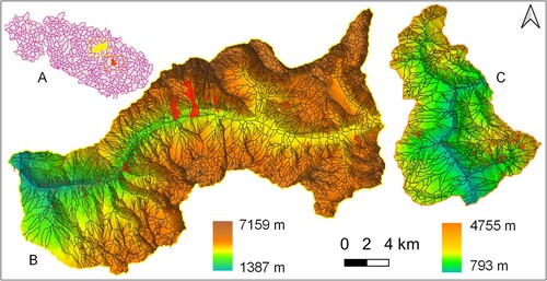
Figure 3 shows an overall view of the area of interest with the location of two selected basins, for which we show details, to allow resolving individual slope unit polygons. The map (B) shows Langtang valley and the map (C) shows a basin in Sindhupalchowk district of Nepal. Langtang is a glaciated valley in higher Himalaya that shook heavily during the 2015 Gorkha earthquake triggering hundreds of landslides including the largest coseismic avalanche, while the Sindhupalchok district lies in the mid hills and receives relatively higher precipitation and landslide number each year during monsoon season ( June–September). In both maps, we show landslides with red polygons, for illustrative purposes; they were induced by earthquake, in (B), and rainfall, in (C).

Figure 3. Slope unit maps in two sample basins selected from the set of basins considered in this work (A); sample basins are located in Langtang area, highlighted in yellow (B), and in the Sinhu area, highlighted in orange (C). Maps (B) and (C) show SU in the two areas. Red polygons show earthquake-induced (B) and rainfall-induced (C) landslides.

Slope units in Langtang and Sinhu basins, Himalaya.

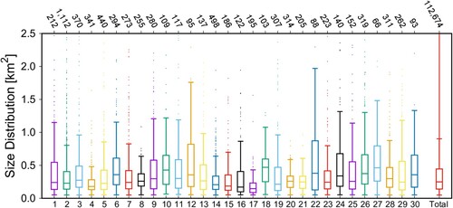
The overall, final SU map is a vector layer, consisting of 112,674 polygons, with an attribute table containing the planimetric area of each polygon and additional morphometric information. The average area of slope units in the map is 0.38 km${}^2$ (minimum area is 49,970 m${}^2$, maximum area is 8.03 km${}^2$, standard deviation 0.42 km${}^2$). Figure 4 shows box plots of the distribution of the size of slope units in a random subset of the individual purple basins of Figure 1, for illustrative purposes, and in the aggregated, final map of Figure 3.

Figure 4. Box plots of the distribution of the size of SU in a subset of 30 purple basins of Figure 1, chosen at random (see also Figure 3), and in the aggregated, final map. The bottom horizontal axis shows a progressive number for the 30 different basins, and the aggregated SU maps (Total); the top horizontal axis shows the number of SU in each set.

Size distributions of slope units in Himalaya.

The map is published with ancillary information, namely an attribute table with mean and standard deviation of morphometric variables, and percentage presence of landforms and thematic variables described in Section 3. Figure 5 shows miniatures of the values of a subset of such variables, one for each variable associated with individual slope units. The full set of variables included in the table distributed with the map is described in Section 6.

Figure 5. Maps of a selection of the variables included in this work, calculated in each SU, either as mean (average, AVG), standard deviation (S.D), percent, presence/absence. A, slope${}_{\mathrm{AVG}}$; B, slope${}_{\mathrm{S}.\mathrm{D}}$; C, elevation${}_{\mathrm{AVG}}$; D, elevation${}_{\mathrm{A}.\mathrm{D}}$; E, relief${}_{\mathrm{AVG}}$; F, relief${}_{\mathrm{STD}}$; G, VRM${}_{\mathrm{AVG}}$; H, VRM${}_{\mathrm{S}.\mathrm{D}}$; I, planar curvature${}_{\mathrm{AVG}}$; J, planar curvature${}_{\mathrm{STD}}$; K, tangential curvature${}_{\mathrm{AVG}}$; L, tangential curvature${}_{\mathrm{STD}}$; M, ‘ridge’${}_{\mathrm{percent}}$; N, ‘slope’${}_{\mathrm{percent}}$ (landform); O, ‘spur’${}_{\mathrm{percent}}$; P, ‘hollow’${}_{\mathrm{percent}}$; Q, ‘valley’${}_{\mathrm{percent}}$; R, $c_{min}^{\mathrm{AVG}}$; S, SU area [km${}^2$]; T, landslide presence (after Roback et al. 2017). Additional variables included in the digital version of the map, published with this work, are described in Section 6.

Spatial distributions of morphometric variables in Himalaya.

4.2. Basin-scale and SU-scale terrain classification

For terrain classification at basin level, we considered purple basins in Figure 1 as spatial aggregation domains. First, we tried to produce a result similar to the terrain classification proposed in Italy by Alvioli et al. (2020). In that case, input variables for k-means were percentiles of the distribution of values of area $a_{min}$ and $c_{min}$ for individual slope units in each basin (as in strategy 1a, in Section 3.2). This strategy produced no sensible result. In fact, using such inputs, we obtained a classification that we could not make sense of, either in terms of topographic nor geo-lithological considerations. We understood this difference as due to an additional level of knowledge used in the previous work, (i.e. basins were first aggregated according to broad physiographic classes); we discarded this result.

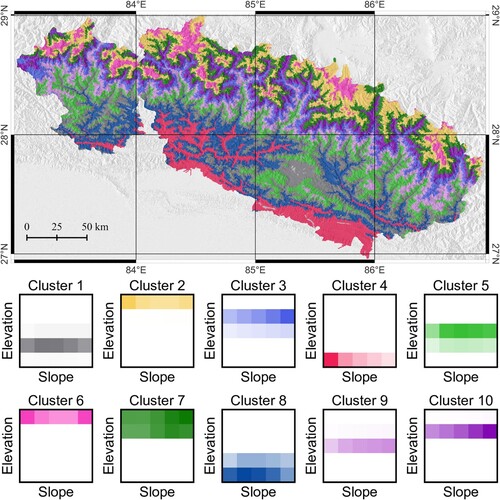
The second arrangement of input variables (morphometric variables, except for area and $c_{min}$; strategy 2a) produced a more interesting result. Figure 6 shows the classification of 450 basins into ten different clusters, denoted with different colors. The boxes below the maps are 2D histograms (joint elevation-slope histograms) with colors matching those in the map; the shade of colors represents the relative frequency of values (darker colors meaning higher values). The subdivision in ten clusters was decided heuristically, after preliminary runs of k-means with a variable number of clusters which revealed that a larger number of clusters would produce redundant classes with similar features.

Figure 6. Top: Unsupervised k-means clustering at basin level, using morphometric and thematic variables, shown in Figure 5. The map contains 10 clusters. Bottom: Joint elevation-slope distribution on the grid cells in each cluster; the color of each box corresponds to one cluster in the top figure; color shade corresponds to the relative frequency of elevation-slope values. The top figure is also included in the supplemental material map.

Terrain classification in Himalaya: basin aggregation level.

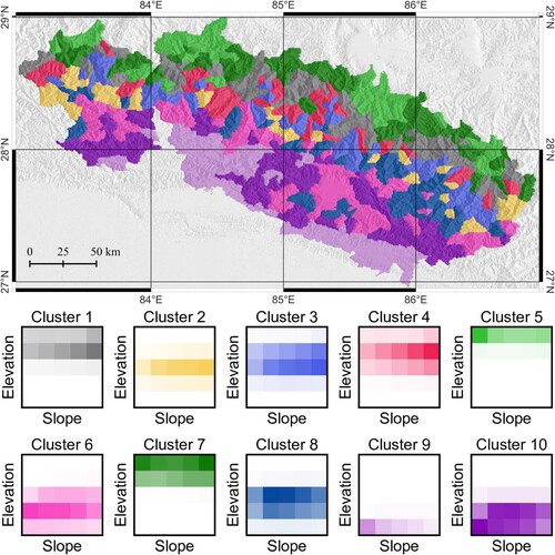
An alternative classification strategy, implemented for the first time in this work, considered SU polygons as spatial aggregation domains. We found the most relevant clustering result, among the six different ones, using all of the morphometric variables except area and mean $c_{min}$ of each slope unit (strategy 1b). Figure 7 shows the outcome of the classification, using ten clusters, as in the case of Figure 6. We note that, in the classification of Figure 7, clusters are mostly correlated with elevation. This is not surprising as in this area large values of relief exist.

Figure 7. Unsupervised k-means clustering at slope unit level, using the same morphometric and thematic variables, but not area and mean $c_{min}$ of each SU. The top figure is the main result of this work, and it is the main map in the supplementary material; the plots in the bottom are included in the supplement as well.

Terrain classification in Himalaya: slope unit aggregation level, result number one.

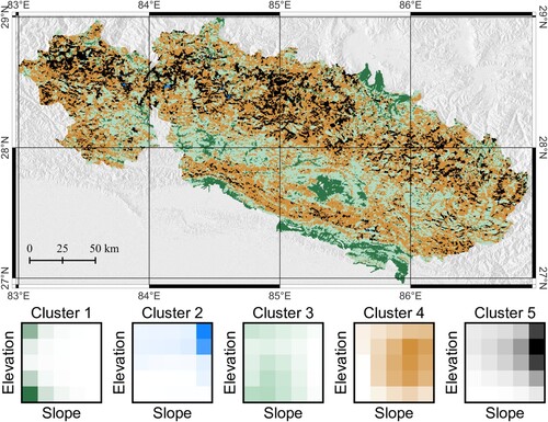
For completeness, we also show the result obtained using the same input variables but elevation (strategy 2b); Figure 8 shows the corresponding map. We selected only five clusters in this case: as a matter of fact, only four of them are represented in the map, since the blue class is seldom found. This result is equally interesting, in our opinion, because there may be applications for which a classification into the five (actually, four) clusters of Figure 8 could be more appropriate than that of Figure 7, if one needs not to consider information about elevation in an explicit way.

Figure 8. As in Figure 7, but removing elevation from clustering, i.e. clustering included all morphometric variables, but not the area, mean $c_{min}$ and elevation of each SU.

Terrain classification in Himalaya: slope unit aggregation level, result number two.

Results of the points 3b–6b were either very similar to the 2b case (3b and 4b), or almost random results (5b and 6b); for illustration purposes, they are shown and discussed in Appendix 1, but we did not consider them interesting enough to be published. In the published SU map, we included three classification schemes resulting from strategies 2a, 1b and 2b corresponding to Figures 6–8.

5. Discussion and conclusion

We presented an SU map of the Himalayas, obtained with state-of-the-art SU delineation and optimization methods. The extent of the area covered by the map delineated for this work, consisting of about 43,000 km${}^2$, required a computationally demanding optimization process, and we only selected the area of interest for the Gorkha earthquake and for the impact of monsoons in Central Nepal. We stress that, since the optimization method relies on a subdivision in hydrological basins, the SU map can be extended in the foreseeable future to basins for which we did not perform optimization yet (see Section 6).

Existing applications of SU maps mainly concern natural hazards; specifically, landslides (Pokharel et al. 2021). For this reason, the collection of variables associated with each SU in the table associated with the map in vector format, we added a binary flag denoting presence/absence of landslides triggered by the Gorkha earthquake contained in three different inventories in the area. We maintain that applications of the proposed map, and of SU in general, may be diverse and interesting.

Terrain classification is a possible application of the map. In this work, we presented various alternative classification strategies, described in Section 3 and whose results are nicely shown in three maps (Figures 6–8). Classification in Figure 6 is fundamentally different with respect to those in Figures 7 and 8. In the first case, classes were assigned to (larger; cf. Figure 1) hydrological basins, while in the second case they are assigned to (much smaller; cf. Figure 3) SU polygons.

Results of terrain classification at basin aggregation level are in Figure 6. The 2D elevation–slope histograms show that the ten different classes are clearly correlated with elevation, and with slope to a lesser degree, similarly to what was shown by Alvioli et al. (2020), in Italy. This was the most interesting result among various attempts to classify individual basins, based on the properties of SU contained therein.

Results of classification of SU level are new to this work and deserve further discussion. The only difference between the two maps presented here is the inclusion of elevation, which was present in Figure 7 and removed in Figure 8. The two results are different: in the first place, the map in Figure 7 admits a larger number of classes (clusters). The elevation–slope histograms below the map in the figure show that most of the classes provide a distinct segmentation in terms of elevation. The classes which could be grouped, had only elevation been considered, are distinct in terms of slope.

For example, we can examine clusters 2 and 6. These encompass areas with very similar elevation, both within the upper division considered in the histograms. Instead, the slope values are different, in that cluster 6 contains steeper slopes than cluster 2. This can be understood, on the one hand, because most of the mountain peaks are in cluster 6 (pink). On the other hand, the smaller values of slope in cluster 2 (yellow) correspond to more gentle relief: this is consistent with the fact that this cluster is mostly located in the northern edge of the study area, in correspondence with the beginning of the Tibetan plateau, and also contain large glaciers.

We did not dig further into the individual contributions from other variables, which were many and diverse, for the sake of simplicity, and relegated alternative classifications to Appendix 1. We stress that classification at SU aggregation level revealed more challenging than at basin level, due to the number and size of polygons involved. This is not related to an increased computational demand related to the number of SU in the maps; the k-means algorithm implemented in R is fast. On the other hand, we found it difficult to find an arrangement of variables used as an input to k-means which produced groups of neighboring polygons classified within the same cluster – elevation and slope aside. As a matter of fact, a cluster with member polygons scattered several kilometers away from each other is arguably not very useful.

On the other hand, classification with k-means initialized with all of the variables used in the previous case, except elevation, provides a substantially different result. Elevation–slope histograms in Figure 8 clearly show a bit fuzzier segmentation, despite the smaller number of classes. This confirms the dominant role of elevation in unsupervised clustering – not surprisingly – and the less relevant role of slope, and other variables. Again, we did not attempt all of the possible combinations of the available variables; a few variations on the theme presented in Section 4 are briefly described in Appendix 1.

The main map in the supplementary material shows the principal result of this work, i.e. the SU map of the area, as in Figure 7. Below the main map, the figures show the SU size distribution, grouped within individual clusters, and slope–elevation distributions, built as two-dimensional normalized histograms; the latter is the same as in Figure 7.

The supplementary material contains, besides the main map, additional maps showing selected morphometric information, and terrain classification at basin level. Smaller maps show: (i) the full collection of 10 landforms (geomorphons), at pixel level; (ii) the average value of elevation, aggregated at SU level; (iii) the average value of slope, aggregated at SU level as well; (iv) alternative terrain classification, at basin level. The difference of pixel-level maps and maps aggregated at basin and SU level is manifest and, in our experience, the latter is useful for geo-spatial analysis on large areas.

We believe that the two different classifications at SU level may be relevant for a variety of applications and represent an interesting step forward, or an alternative, with respect to grid-based classification. Although the latter has a higher resolution, the congruence of SU polygons with natural landforms (i.e. hill slopes, defined by scale-dependent drainage and divide lines) makes the former easier to interpret in morphological terms and gives advantages for terrain classification, analysis and visualization.

Geolocation information

The map proposed in this work is encompassed by the bounding box: 26:57:26.5N–29:00:00.5N, 82:59:59.5E–86:54:33.5E (EPSG:4326), mostly in Nepal.

Software

All of the analyses described in this work were performed in GRASS GIS running in a Linux OS, using extensive bash scripting and parallel computing. The main slope unit delineation was performed using the r.slopeunits module, by Alvioli et al. (2016); Table 1 lists details about additional specific software modules and references. Figures were prepared using QGIS (maps) and using Gnuplot (plots). The whole manuscript was typesetted using LaTeX, including the supplemental map.

Table 1. Description of the content of the table associated with the slope unit map. References may refer to the original work where a software tool was developed, where the concept was introduced and/or used in a context similar to the present one, or to where data was extracted from.

Field	Description	Units	Software	Reference
su_area	area of the polygon	[m${}^2$]	–	–
cvar_avg	mean circular variance	–	r.mapcalc	Alvioli et al. (2016)
elev_avg	mean elevation	[m]	–	https://bhuvan.nrsc.gov.in
elev_sd	S.D of elevation	[m]	–
relief_avg	mean elevation range	[m]	r.neighbors	–
relief_sd	S.D of relief	[m]
slope_avg	mean slope	[deg]	r.slope.aspect	Hofierka et al. (2009)
slope_sd	S.D of slope	[deg]
pcurv_avg	mean planar curvature	[m${}^{-1}$]
pcurv_sd	S.D of planar curvature	[m${}^{-1}$]
tcurv_avg	mean transversal curvature	[m${}^{-1}$]
tcurv_sd	S.D transversal curvature	[m${}^{-1}$]
vrm_avg	av. vector ruggedness measure	–	r.vector.ruggedness	Sappington et al. (2007)
vrm_sd	S.D of VRM	–
twi_avg	av. topographic wetness index	–	r.topidx	–
twi_sd	S.D of TWI	–
form_valley	percent of ‘valley’ landform	–	r.geomorphon	Jasiewicz and Stepinski (2013)
form_ridge	percent of ‘ridge’ landform	–
form_spur	percent of ‘spur’ landform	–
form_slope	percent of ‘slope’ landform	–
form_hollow	percent of ‘hollow’ landform	–
annual_rain	mean annual precipitation	[mm/y]	–	Funk et al. (2015)
daily_rain	mean daily precipitation	[mm/d]
Field	Description
cat	unique SU polygon identifier
glim_code	dominant geology, using GLiM codes from Hartmann and Moosdorf (2012)
landslides	landslide presence/absence (given as 1/0), using polygons from Roback et al. (2017)
cluster_basin	cluster classification at basin level (cf. point 2a Section 3.2 and Figure 6)
cluster_su_A	cluster classification at slope unit level (cf. point 1b Section 3.2 and Figure 7)
cluster_su_B	cluster classification at slope unit level (cf. point 2b Section 3.2 and Figure 8)
basin	unique basin identifier: allows recovering the purple basins of Figure 1

Disclosure statement

No potential conflict of interest was reported by the authors.

Data availability statement

The slope unit map introduced in this work is available for download at the main slope units project page, on the CNR IRPI web server: http://geomorphology.irpi.cnr.it/tools/slope-units. We distribute the map in OGC GeoPackage vector format (readable by most GIS software); reference system is EPSG:4326.

The attribute table contains the fields listed in Table 1. Among the fields listed in the table, only a few were used for terrain classification, as explained in detail in Section 3.2. The remaining fields, such as mean annual and daily rainfall, geological GLiM code, landslide presence and TWI, were added to enrich the content of the published map. Eventually, the three cluster_⋆ fields are the results of the classification proposed in this work as an application of the map. A few of these fields are shown explicitly in the maps in Figure 5. The four additional classification results described in Appendix 1 are available upon request.

Additional information

Funding

B.P. thanks the Australian Government Research Training Program at the University of New South Wales, Australia, for sponsoring her research. K.G. thanks the University of British Columbia for sponsoring his research. B.P. thanks the HPC-Europa3 consortium for a mobility grant and use of HPC facilities, and CNR IRPI, Perugia, Italy, for hospitality.

Notes

1 The SRTM tiles used in this work are: N26E83, N26E84, N26E85, N26E86, N27E83, N27E84, N27E85, N27E86, N28E83, N28E84, N28E85, N28E86, N29E83, N29E84, N29E85.

Appendix 1.

Alternative k-means classifications

In Section 3, we described different strategies for terrain classification in the area of interest. The differences between the various strategies were (i) spatial aggregation domains and (ii) variables fed to the k-means algorithm, for actual classification. Considering hydrological basins as aggregation domains, we found a consistent terrain classification using as an input all of the morphometric variables calculated within SU polygons; actual inputs where their mean values, at basin level. On the other hand, classification at SU level revealed a bit more challenging and required experimenting different combinations of variables to obtain consistent results. Figures 7 and 8 show two different classifications, with ten and five clusters, respectively.

Here, we show four further variations on those two approaches, i.e. four additional combinations of input variables, corresponding to the following points, already described in Section 3:

Terrain classification in Himalaya: slope unit aggregation level, alternative results.

Figure A1. Clustering of individual slope units, using the different approximations (3b)–(6b) listed in Section 3.2 and described in Appendix A. (a) Corresponding to strategy (3b): as in Figure 7, but removing elevation and slope from clustering, i.e. clustering included all morphometric variables, but not the area, mean $c_{min}$, slope and elevation of each SU. (b) Strategy (4b): as in (a), but adding mean $c_{min}$; there is no sensible change in the results. (c) Strategy (5b): clustering of individual SU, using only mean $c_{min}$ as a variable. The pattern of the different cluster looks random, and the number of clusters is redundant, as shown in the slope-elevation 2D histograms. (d) Strategy (6b): only the mean $c_{min}$ of each SU was used for clustering; in this case, we used three clusters.

(3b)	all morphometric variables, excluding elevation and slope; the resulting classified map is in Figure A1(a). The results are very similar to the one of point 2b, though minor differences could be spotted.
(4b)	as in (3b), except adding mean $c_{min}$; the resulting classified map is in Figure A1(b). Same comment as above.
(5b)	k-means classification using only the area and mean $c_{min}$ of each SU; the resulting map is in Figure A1(c). The map shows an almost completely random pattern, making it useless for any further discussion. The figure shows the typical output of classification attempted with many other combinations of input variables, if we leave out most of the morphometric variables.
(6b)	k-means classification using only mean $c_{min}$ of each SU, and using only three clusters; the resulting map is in Figure A1(d). Conclusion is similar to the ones of point (5b).

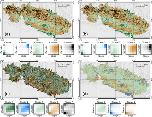One last comment is that the use of mean $c_{min}$ is almost irrelevant is an indication that there is no memory of the optimization procedure, in individual slope units. In fact, results of strategies 4b–6b show that $c_{min}$ only produces a pattern in k-means classification when used alone.

Appendix 2.

Description of the printable map

The map proposed in this work consists of 112,674 slope units polygons of varying shape and size, covering a total area of about 43,000 km${}^2$, mostly in Nepal (inset within the main map), and it is intended for printing in A3 format. The main map is also distributed in digital format (cf. Section 6).

As the average area of the polygons is below 0.5 km${}^2$, with many outliers (cf. boxplots of SU size distributions), a graphical representation of the whole area would necessarily be unable to show details of individual polygons. To cope with that and present an appealing map, we show one of the applications of the polygonal map proposed in our work, i.e. a terrain classification in ten clusters. The main map in the supplement shows such classification, in ten clusters, with 10 different colors. Matching colors are used to show the distribution of the size of slope units within each cluster and two-dimensional histograms of values of elevation and slope, within each cluster as well (shown in the plots below the main map). From the main map, the reader can appreciate the aggregation at slope unit level – one of the main result of the proposed work – and have a good grasp on the spatial distribution of slope unit polygons, though the boundaries of individual polygons can only be appreciated on the digital map.

To give further insight on the meaning of aggregation of spatial variables at slope unit level, we included four additional figures in the supplemental map, on the right. From top to bottom: the first one shows specific quantities at pixel level (00:00:01 degree resolution), namely landforms. The second and third maps show, respectively, elevation and slope values at the slope unit aggregation level (mean values). Eventually, the fourth map shows terrain classification at the basin level – an additional result from this work.

We believe that the supplemental map accomplishes the aim of (i) being self-contained, (ii) representing the difference between pixel, slope unit and basin level, and (iii) summarizing the main results of the proposed work.

References

- Alvioli, M., Guzzetti, F., & Marchesini, I. (2020). Parameter-free delineation of slope units and terrain subdivision of Italy. Geomorphology, 358(9), 107124. https://doi.org/10.1016/j.geomorph.2020.107124.
- Alvioli, M., Marchesini, I., Reichenbach, P., Rossi, M., Ardizzone, F., Fiorucci, F., & Guzzetti, F. (2016). Automatic delineation of geomorphological slope units with r.slopeunits v1.0 and their optimization for landslide susceptibility modeling. Geoscientific Model Development, 9(11), 3975–3991. https://doi.org/10.5194/gmd-9-3975-2016.
- Alvioli, M., Mondini, A. C., Fiorucci, F., Cardinali, M., & Marchesini, I. (2018). Topography-driven satellite imagery analysis for landslide mapping. Geomatics, Natural Hazards and Risk, 9(1), 544–567. https://doi.org/10.1080/19475705.2018.1458050.
- Alvioli, M., Santangelo, M., Fiorucci, F., Cardinali, M., Marchesini, I., Reichenbach, P., Rossi, M., Guzzetti, F., & Peruccacci, S. (2021). Rockfall susceptibility and network-ranked susceptibility along the Italian railway. Engineering Geology, 293(3), 106301. https://doi.org/10.1016/j.enggeo.2021.106301.
- Amato, G., Fiorucci, M., Martino, S., Lombardo, L., & Palombi, L. (2020, January). Earthquake-triggered landslide susceptibility in Italy by means of artificial neural network. https://doi.org/10.31223/X59W39.
- Belgiu, M., & Drăguţ, L. (2016). Random forest in remote sensing: A review of applications and future directions. ISPRS Journal of Photogrammetry and Remote Sensing, 114(Part A), 24–31. https://doi.org/10.1016/j.isprsjprs.2016.01.011.
- Bornaetxea, T., Rossi, M., Marchesini, I., & Alvioli, M. (2018). Effective surveyed area and its role in statistical landslide susceptibility assessments. Natural Hazards and Earth System Sciences, 18(9), 2455–2469. https://doi.org/10.5194/nhess-18-2455-2018.
- Camilo, D. C., Lombardo, L., Mai, P. M., Dou, J., & Huser, R. (2017). Handling high predictor dimensionality in slope-unit-based landslide susceptibility models through lasso-penalized generalized linear model. Environmental Modelling & Software, 97(1), 145–156. https://doi.org/10.1016/j.envsoft.2017.08.003.
- Chen, Z., Liang, S., Ke, Y., Yang, Z., & Zhao, H. (2020). Landslide susceptibility assessment using different slope units based on the evidential belief function model. Geocarto International, 35(15), 1641–1664. https://doi.org/10.1080/10106049.2019.1582716.
- Cook, K. L., Andermann, C., Gimbert, F., Adhikari, B. R., & Hovius, N. (2018). Glacial lake outburst floods as drivers of fluvial erosion in the Himalaya. Science (New York, NY), 362(6410), 53–57. https://doi.org/10.1126/science.aat4981.
- Doménech, G., Alvioli, M., & Corominas, J. (2020). Preparing first-time slope failures hazard maps: from pixel-based to slope unit-based. Landslides, 17(2), 249–265. https://doi.org/10.1007/s10346-019-01279-4.
- Drăguţ, L., & Blaschke, T. (2006). Automated classification of landform elements using object-based image analysis. Geomorphology, 81(3–4), 330–344. https://doi.org/10.1016/j.geomorph.2006.04.013.
- Espindola, G. M., Câmara, G., Reis, I. A., Bins, L. S., & Monteiro, A. M. (2006). Parameter selection for region-growing image segmentation algorithms using spatial autocorrelation. International Journal of Remote Sensing, 14(14), 3035–3040. https://doi.org/10.1080/01431160600617194.
- Falcone, G., Acunzo, G., Mendicelli, A., Mori, F., Naso, G., Peronace, E., Porchia, A., Romagnoli, G., Tarquini, E., & Moscatelli, M. (2021). Seismic amplification maps of Italy based on site-specific microzonation dataset and one-dimensional numerical approach. Engineering Geology, 289, 106170. https://doi.org/10.1016/j.enggeo.2021.106170.
- Funk, C., Peterson, P., Landsfeld, M., Pedreros, D., Verdin, J., Shukla, S., Husak, G., Rowland, J., Harrison, L., Hoell, A., & Michaelsen, J. (2015). The climate hazards infrared precipitation with stations – A new environmental record for monitoring extremes. Scientific Data, 2(1), 150066. https://doi.org/10.1038/sdata.2015.66.
- Gnyawali, K. R., & Adhikari, B. R. (2017). Spatial relations of earthquake induced landslides triggered by 2015 Gorkha earthquake Mw = 7.8. In M. Mikoš, N. Casagli, Y. Yin, and K. Sassa (Eds.), Advancing culture of living with landslides (pp. 85–93). Springer International Publishing. ISBN 978–3–319–53485–5.
- Hartigan, J. A., & Wong, M. A. (1979). Algorithm AS 136: A k-means clustering algorithm. Journal of the Royal Statistical Society. Series C (Applied Statistics), 28(1), 100–108. https://doi.org/10.2307/2346830.
- Hartmann, J., & Moosdorf, N. (2012). The new global lithological map database GLiM: A representation of rock properties at the Earth surface. Geochemistry, Geophysics, Geosystems, 13(12), 119. https://doi.org/10.1029/2012GC004370.
- Heckmann, T., Cavalli, M., Cerdan, O., Foerster, S., Javaux, M., Lode, E., Smetanová, A., Vericat, D., & Brardinoni, F. (2018). Indices of sediment connectivity: opportunities, challenges and limitations. Earth–Science Reviews, 187(12), 77–108. https://doi.org/10.1016/j.earscirev.2018.08.004.
- Hofierka, J., Mitášová, H., & Neteler, M. (2009). Chapter 17 geomorphometry in grass gis. In T. Hengl and H. I. Reuter (Eds.), Geomorphometry, Vol. 33 of Developments in soil science (pp. 387–410). Elsevier. https://doi.org/10.1016/S0166-2481(08)00017-2.
- Iwahashi, J., Kamiya, I., Matsuoka, M., & Yamazaki, D. (2018, January). Global terrain classification using 280 m dems: Segmentation, clustering, and reclassification. Progress in Earth and Planetary Science, 5(1), 1. https://doi.org/10.1186/s40645-017-0157-2.
- Iwahashi, J., & Yamazaki, D. (2021). Global polygons for terrain classification divided into uniform slopes and basins. Preprint.
- Jacobs, L., Kervyn, M., Reichenbach, P., Rossi, M., Marchesini, I., Alvioli, M., & Dewitte, O. (2020). Regional susceptibility assessments with heterogeneous landslide information: Slope unit- vs. pixel-based approach. Geomorphology, 356, 107084. https://doi.org/10.1016/j.geomorph.2020.107084.
- Jasiewicz, J., & Stepinski, T. F. (2013). Geomorphons -- A pattern recognition approach to classification and mapping of landforms. Geomorphology, 182(10), 147–156. https://doi.org/10.1016/j.geomorph.2012.11.005.
- Kargel, J. S., Leonard, G. J., Shugar, D. H., Haritashya, U. K., Fielding, E. J., Bevington, A., Fujita, K., Geertsema, M., Miles, E. S., Steiner, J., Bajracharya, S., Anderson, E., Bawden, G. W., Breashears, D. F., Byers, A., Collins, B., Donnellan, A., Dhital, M. R., Evans, T. L., … Young, N. (2016). Geomorphic and geologic controls of geohazards induced by Nepal's 2015 Gorkha earthquake. Science (New York, NY), 351(6269), aac8353. https://doi.org/10.1126/science.aac8353.
- López-Vinielles, J., Fernández-Merodo, J. A., Ezquerro, P., García-Davalillo, J. C., Sarro, R., Reyes-Carmona, C., Barra, A., Navarro, J. A., Krishnakumar, V., Alvioli, M., & Herrera, G. (2021). Combining satellite insar, slope units and finite element modeling for stability analysis in mining waste disposal areas. Remote Sensing, 13(10). https://doi.org/10.3390/rs13102008.
- Li, L., & Lan, H. (2020). Integration of spatial probability and size in slope–unit–based landslide susceptibility assessment: A case study. International Journal of Environmental Research and Public Health, 17(21), 8055. https://doi.org/10.3390/ijerph17218055.
- Marc, O., Behling, R., Andermann, C., Turowski, J. M., Illien, L., Roessner, S., & Hovius, N. (2019). Long-term erosion of the Nepal Himalayas by bedrock landsliding: The role of monsoons, earthquakes and giant landslides. Earth Surface Dynamics, 7(1), 107–128. https://doi.org/10.5194/esurf-7-107-2019.
- Marchesini, I., Salvati, P., Rossi, M., Donnini, M., Sterlacchini, S., & Guzzetti, F. (2021). Data-driven flood hazard zonation of Italy. Journal of Environmental Management, 294(11), 112986. https://doi.org/10.1016/j.jenvman.2021.112986.
- Mazzoglio, P., Butera, I., Alvioli, M., & Claps, P. (2022). The role of morphology on the spatial distribution of short-duration rainfall extremes in Italy. Hydrology and Earth System, 26, 1659–1672. https://doi.org/10.5194/hess-26-1659-2022
- Minár, J., & Evans, I. S. (2008). Elementary forms for land surface segmentation: The theoretical basis of terrain analysis and geomorphological mapping. Geomorphology, 95(3–4), 236–259. https://doi.org/10.1016/j.geomorph.2007.06.003.
- Mori, F., Mendicelli, A., Moscatelli, M., Romagnoli, G., Peronace, E., & Naso, G. (2020). A new Vs30 map for Italy based on the seismic microzonation dataset. Engineering Geology, 275, 105745. https://doi.org/10.1016/j.enggeo.2020.105745.
- Panagos, P., Van Liedekerke, M., Jones, A., & Montanarella, L. (2012). European soil data centre: Response to European policy support and public data requirements. Land Use Policy, 29(2), 329–338. https://doi.org/10.1016/j.landusepol.2011.07.003.
- Pokharel, B., Alvioli, M., & Lim, S. (2020). Relevance of morphometric parameters in susceptibility modelling of earthquake-induced landslides. In M. Alvioli, I. Marchesini, L. Melelli, P. Guth, and S. Peckham, (Eds), Proceedings of the sixth Geomorphometry conference: Geomorphometry 2020. CNR Edizioni. https://doi.org/10.30437/geomorphometry2020_49.
- Pokharel, B., Alvioli, M., & Lim, S. (2021). Assessment of earthquake-induced landslide inventories and susceptibility maps using slope unit-based logistic regression and geospatial statistics. Scientific Reports, 11(1), 21333. https://doi.org/10.1038/s41598-021-00780-y.
- Roback, K., Clark, M. K., West, A. J., Zekkos, D., Li, G., Gallen, S. F., Chamlagain, D., & Godt, J. W. (2018). The size, distribution, and mobility of landslides caused by the 2015 Mw7.8 Gorkha earthquake, Nepal. Geomorphology, 301(B4), 121–138. https://doi.org/10.1016/j.geomorph.2017.01.030.
- Roback, K., Clark, M. K., West, A. J., Zekkos, D., Li, G., Gallen, S. F., Champlain, D., & Godt, J. W. (2017). Map data of landslides triggered by the 25 April 2015 Mw 7.8 Gorkha, Nepal earthquake. U.S. Geological Survey data release.
- Sappington, J. M., Longshore, K. M., & Thompson, D. B. (2007). Quantifying landscape ruggedness for animal habitat analysis: A case study using bighorn sheep in the Mojave Desert. Journal of Wildlife Management, 71(5), 1419–1426. https://doi.org/10.2193/2005-723.
- Schlögel, R., Marchesini, I., Alvioli, M., Reichenbach, P., Rossi, M., & Malet, J.-P. (2018). Optimizing landslide susceptibility zonation: Effects of DEM spatial resolution and slope unit delineation on logistic regression models. Geomorphology, 301(1), 10–20. https://doi.org/10.1016/j.geomorph.2017.10.018.
- Tanyaş, H., Rossi, M., Alvioli, M., van Westen, C. J., & Marchesini, I. (2019). A global slope unit-based method for the near real-time prediction of earthquake-induced landslides. Geomorphology, 327(2), 126–146. https://doi.org/10.1016/j.geomorph.2018.10.022.
- Tanyaş, H., van Westen, C. J., Persello, C., & Alvioli, M. (2019, April). Rapid prediction of the magnitude scale of landslide events triggered by an earthquake. Landslides, 16(4), 661–676. https://doi.org/10.1007/s10346-019-01136-4.
- Zhang, J.-Q., Liu, R.-K., Deng, W., Khanal, N. R., Gurung, D. R., Murthy, M. S. R., & Wahid, S. (2016). Characteristics of landslide in Koshi River Basin, Central Himalaya. Journal of Mountain Science, 13(10), 1711–1722. https://doi.org/10.1007/s11629-016-4017-0.