Quantifying and visualizing 32 years of agricultural land use change in Kabul, Afghanistan

ABSTRACT

Agriculture is a key element of Afghanistan’s economy and plays an essential role supporting the expanding population and urban development of Kabul, the country’s capital. Over the past decades the urban landscape has changed substantially and agricultural land use has shifted in its extent, location, and density. Identifying trends in the amount of agricultural area, as an indication of food production, is important for city planning and humanitarian efforts. While many studies have investigated Afghanistan's agriculture, most are conducted at scales that preclude their use for local-scale decision-making. This study quantifies agricultural extent across 32 years from 1988 to 2020 at local scale using simple and repeatable Landsat multispectral image analysis. The volume of data in time-series analysis complicatesvisualization of key findings and long-term trends. This study also explored visualization methods such as zonal mapping, animations, and the isolation of key themes in a 2D static map.

KEYWORDS:

• Agriculture
• land-use change
• Kabul Afghanistan
• time-series visualization
• change detection

1. Introduction

Agriculture is a significant part of Afghanistan’s economy, employing a large percentage of the nation’s workforce, accounting for nearly 60% of the total licit exports, and making up approximately a quarter of the national GDP (FAO 2018). Near the capital city of Kabul agricultural production is key to feeding the city’s population, which has grown from less than 2 million in the late 1970s to a recent estimate of over 4.2 million in 2020 (The World Factbook, 2020). Farming in this region is primarily small-scale, with an average farm size of 0.4 ha, and land rental through sharecropping is common (Safi et al., 2011). In the city and peri-urban spaces of Kabul, small vegetable crops are largely grown for household or community consumption, while larger cereal crops are grown in more rural areas (Safi et al., 2011). Over the past three decades, agricultural land use in this region has substantially changed in extent, location, and density to accommodate the city’s growth and changing socio-political situation (Najmuddin et al., 2018; United Nations, 2018). More importantly, the means of irrigating crops has fundamentally shifted from redirection of snow-fed mountain runoff to groundwater pumping (Maletta, 2007; Ghulami, 2017).

There is substantial literature describing Afghanistan’s agricultural production in terms of its contribution to the economic sector (Khaliq & Boz, 2018), its effect on national recovery (Kawasaki et al., 2012), and its contribution to rural development (Pain & Shah, 2009); however, the bulk of these investigations have been conducted at the national scale (Tiwari et al., 2020; Pervez et al., 2014), focus primarily on illicit crops such as poppy cultivation (Jones et al., 2019), and do not produce data that enables local-scale policy and management decisions. Moreover, the methods of many investigations of agriculture hinge significantly on image acquisition during the peak of growing season to map healthy mature crops (Pan et al., 2015; Pervez et al., 2014). The results of such analyses do not account for fallow or recently-planted agricultural areas. Additionally, previous studies about agriculture in Afghanistan do not include geospatial datasets that enable re-application of agricultural findings for other investigative or management purposes.

This study aimed to quantify the extent and location of agricultural areas in the greater Kabul area over 32 years from 1988 to 2020. An essential objective of this work was to use simple, repeatable, and automated analysis of freely available satellite imagery to map agricultural area at the local scale. To accomplish this goal, multispectral imagery from the Landsat satellite was analyzed using band ratio analysis to map both growing and fallow agricultural areas.

Time-series land cover change analyses produce results that integrate the dimension of time with the two-dimensional (2D) space (e.g. latitude and longitude). Due to the limitations of traditional 2D mapping and the density of time series data, these results must be conveyed either through multiple maps – each representing a snapshot of the time series – or be reduced to statistical or graph form (Ott & Swiaczny, 2001). While the visualization of data using multiple maps – one per year of analysis – is a commonly adopted method of displaying change analysis results (Hawbaker et al., 2017), this method is ineffective at communicating results when many dates of observation – or years – are included in the analysis. Conveyance of results using a graph requires significant generalization of results (Chang et al., 2007) and neglects the geospatial distribution of results that can be visualized in a map format (Pătru-Stupariu et al., 2011). Thus, the third objective of this study was to develop a method to visualize 30 years of agricultural change in a traditional 2D map.

2. Materials and methods

2.1. Study area

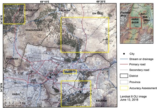
The area of interest includes the city of Kabul in the Kabul district, and encompasses the urban and peri-urban sprawl that radiates into neighboring districts of Dih Sabz, Bagrami, Shakardara, Paghman, and Mir Bacha Kot (Figure 1). This metropolitan area lies within the Kabul basin, a valley formed by the Paghman Mountains to the west and the Koh-i-Sofe Mountains to the east. The basin has a semi-arid continental climate that receives an average, though highly variable, annual precipitation of 330 mm, (Tünnermeier & Houben, 2005). Most of this precipitation falls as snow in the surrounding mountains during winter months, which subsequently recharges the Paghman, Logar, and Kabul rivers in spring. These rivers gradually run dry during warm dry summer months. Snow melt also recharges the aquifers associated with each of the rivers, which are used in the late summer to irrigate fields (Tünnermeier & Houben, 2005). While the area is underlain by a complex system of 3 different layers of aquifer (Mack and others 2014), recharge in the Kabul basin is largely unable to compensate for agricultural and other anthropogenic drawdown and evapotranspiration (Taher et al., 2014). Water quality and water table height are generally lower in Kabul than in its surrounding rural environs (Broshears et al., 2005).

Figure 1. Study area figure.

Map of study area around Kabul, Afghanistan. Within this area, 4 yellow-outline boxes denote the extent of accuracy assessment.

2.2. Data

Landsat multispectral images were acquired on near-anniversary dates at the height of the growing season, between 1988 and 2020. Due to cloud coverage or gaps in the image record, an appropriate image was not available for nine of the years during this 32-year time period. In total 24 different Landsat images (listed in Table 1) were used in the analysis. Additionally, very high-resolution images acquired by the WorldView-2 satellite on 2 November 2017 were used to assess the accuracy of analysis results.

Table 1. Landsat images used in annual NDVI analysis; NA indicates that an image was not available during the growing season with low cloud coverage.

Year	Sat/Sensor	Acquisition date
1988	L5 TM	05/09/1988
1989	–	NA
1990	L5 TM	5/15/1990
1991	–	NA
1992	L5 TM	5/4/1992
1993	L5 TM	5/23/1993
1994	L5 TM	5/10/1994
1995	L5 TM	5/13/1995
1996	L5 TM	5/15/1996
1997	L5 TM	5/18/1997
1998	L5 TM	5/21/1998
1999	L5 TM	5/8/1999
2000	L5 TM	5/10/2000
2001	L5 TM	5/13/2001
2002	L5 TM	5/16/2002
2003	L7 ETM+	5/11/2003
2004	–	NA
2005	–	NA
2006	–	NA
2007	–	NA
2008	L5 TM	5/16/2008
2009	–	NA
2010	–	NA
2011	L5 TM	5/25/2011
2012	–	NA
2013	L8 OLI	5/14/2013
2014	L8 OLI	5/1/2014
2015	L8 OLI	5/20/2015
2016	L8 OLI	5/22/2016
2017	L8 OLI	5/25/2017
2018	L8 OLI	6/13/2018
2019	L8 OLI	5/30/2019
2020	L8 OLI	6/18/2020

2.3. Band ratio analysis

Most of the moderate-scale satellite multispectral image analysis methods used to map the extent of agriculture focus on the identification of healthy growing crops. This is achieved through isolation of an absorption feature in red wavelengths caused by the chlorophyll pigments of healthy vegetation (Jensen, 2007). While there are many variations of vegetation indices which account for factors such as varying amounts of foliage cover (Haboudane et al., 2002), water moisture (Huang et al., 2002), and illumination conditions, the reliance of all on the presence of green vegetation means that fields without growing vegetation are not included in the detected cultivated land. This results in a substantial underestimation of the total cultivated area.

In this study a compound band ratio analysis was developed, wherein a vegetation index was combined with a band ratio commonly used to highlight clay and other fine-particle soils. The soil-adjusted vegetation index (SAVI), was selected because it has been shown to be successful in quantifying vegetation in arid landscapes where soil shows through the foliage (Huete, 1988). For each image, SAVI was calculated using the equation $SAVI={\displaystyle \frac{(NIR-Red)}{(NIR+Red+L)}\times (1+L),}$where L is a value indicating the amount of green vegetative cover. Selection of an L value depends on the amount of vegetative cover, where L = 1 should be adopted for areas with no green vegetation, and L = 0 should be adopted for areas with lush dense vegetative cover (Huete, 1988). Since the arid environment of Kabul promotes the natural growth of sparse green vegetation, a value of 0.75 was used for L.

Next, a clay index (Boettinger et al., 2008) was selected because of its success in highlighting the fine soil particles of Kabul’s wind-blown loess deposits (DeWitt et al., 2021). This clay band ratio was calculated for each image using the equation $ClayBandRatio={\displaystyle \frac{(SWIR1-SWIR2)}{(SWIR1+SWIR2)}}$Summary statistics (minimum, maximum, mean, standard deviation) of the SAVI and clay band ratio results for each year of analysis were then calculated for the study area.

The above methods were scripted to improve the efficiency of data analysis and to reduce the potential of human error in the processing of 24 images. The scripts were written in the integrated development environment PyCharm by JetBrains. The python site package ArcPy was used to access the ArcGIS toolbox functions. The processes that were scripted and completed by using ArcPy include geodatabase creation, table conversions, data clipping, band ratio analyses, and statistic computations among a few other environment setting commands. The output of these scripts were new raster data and tables containing global or zonal statistics. The scripts written for the analysis are published in Appendix A.

In order to differentiate between cultivated areas and all other areas in the band ratio results, a unique threshold was identified for the SAVI and the clay band ratio results for each year. It was determined that a threshold value of the band ratio mean (within the study area) plus 1 standard deviation consistently distinguished between cultivated and other areas in each band ratio result. In both the SAVI and the clay band ratio results, values above the threshold correspond to dense and healthy growing crops or to bare soil with fine grain size and high clay content (respectively). Values below the threshold correspond to all other areas. Reclassification of the SAVI and clay band ratio results generated two new images for each year of analysis, where areas of dense green vegetation or bare tilled soil (respectively) were given a value of 1 and all other areas were given a value of 0. The two reclassified rasters were then added together to fully characterize agricultural areas – both healthy vegetation and bare fields. In the result, values of 0 = not agricultural area, 1–2 = fallow or vegetated agricultural fields, and this result was then reclassified so that all values greater than zero were given a value of 1. Zonal statistics based on district boundaries were then calculated for each year to quantify the extent of agriculture within each district in each year.

The accuracy of the combined band ratio analysis for 2017 was assessed globally within the extent of the accuracy assessment areas (Figure 1) by comparison to areas of agriculture manually interpreted from very high-resolution satellite imagery acquired on 11/6/2017. Together, the four accuracy assessment areas cover 25% of the study area. The vector-based areas of agriculture interpreted from the reference imagery were converted to a 30 m raster (hereafter referred to as ‘reference raster’), where gridcells covering an agricultural area were given a value of 100 and gridcells covering all other areas were given a value of 200. The 2017 combined band ratio result was then added to the reference raster, and the count of each assessment gridcell value was compiled into a confusion matrix. The possible outcomes of the assessment are shown in Table 2. The producer’s, user’s, and overall accuracy were calculated from the confusion matrix (Table 3).

Table 2. Possible gridcell values of the accuracy assessment.

Accuracy gridcell value	Meaning
	BR Analysis indicates that the area is …	Reference raster indicates the area is …
100	Not agriculture	Agriculture
101	Agriculture	Agriculture
200	Not agriculture	Not agriculture
201	Agriculture	Not agriculture

Table 3. Accuracy assessment results.

	Producer’s	User’s
Agriculture	75.5%	84.3%
Not agriculture	93.0%	88.4%
Overall accuracy	87.1%

2.4. Visualization of change

While the annual agricultural area resultant from the combined band ratio analysis is useful for management or policy mapping purposes, it is difficult to visualize overarching trends from 24 years of detailed map results. More importantly, the nuanced, geospatial changes that occur between each year of the analysis are muted by the volume of visual data conveyed by the time series. To improve visualization of these changes and trends over time, the result for each year was generalized to a 1 square kilometer grid. The value of each gridcell reflects the area of agriculture mapped within the 1 square kilometer cell, calculated as $gridcellvalue=countofagriculturepixels\times 900{\mathrm{m}}^2$The 24 results of this zonal mapping were individually mapped using a white to green color ramp with 4 classes to show the area of agriculture in each zone. Zones with very small agricultural extent (<250,001 km²) were effectively ‘masked’ from the map by using white color; zones with small (250,001–500,000 km²) or medium (500,000–750,000 km²) agricultural areas were colored light or medium green; zones with large agricultural area (750,000–100,000 km²) were colored dark green. These 24 result maps were compiled into an animation using TechSmith Camtaisa to enable visualization of changes over time. Each of the animation frames shows a single map, organized from oldest (1988) to newest (2020), which appears in the frame for 0.20 s × the number of years between it and the next map result. In this way the viewer will understand that there may be multi-year gaps between frames of the results.

A single two-dimensional (2D) map was created to show the results of 32 years of agricultural change. The results of the band ratio zonal analyses were further synthesized down to identify the maximum extent of agricultural area in each gridcell over the 32 years of analysis. Additionally, the year in which this maximum extent occurred in each gridcell was also derived from the zonal results. These two factors were combined together in a static map using different color ramps and partial transparency. The maximum agricultural extent was given a yellow to dark red color ramp, and the year of maximum agricultural extent was given a magenta to cyan color ramp.

3. Results

3.1. Band ratio analysis results

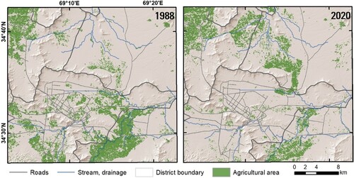
The results of the combined band ratio analysis for 2020 are shown in Figure 2. The area of detail shows that the SAVI and the clay band ratios identify different, but adjacent areas. Together these adjacent areas describe the extent of cultivated land. Figure 3 shows the final result of this procedure, where the combined band ratio result was reclassified to a single class of ‘agricultural area’. In this figure, the 1988 and 2020 results are shown side by side to allow for comparison of the agricultural areas across 32 years of change, however it should be noted that 24 individual maps were created of the results.

Figure 2. Results of the combined band ratio analysis.

Map of combined band ratio analysis results. Extent of fields with growing crop is shown in green and extent of fallow fields with vegetation are shown in orange. An area of detail map shows a zoomed in area of these results in the Dih Sabz district.

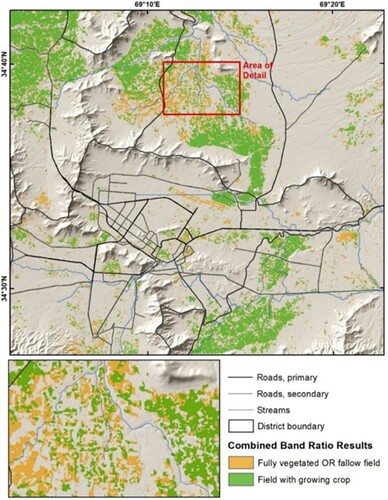
Figure 3. Results of combined band ratio analysis, indicating ‘agricultural area’ for 1988 and 2020.

Two map frames show the results of the combined band ratio analysis for 1988 (left frame) and 2020 (right frame). Agricultural area is indicated by the extent of combined band ratio analysis in each frame.

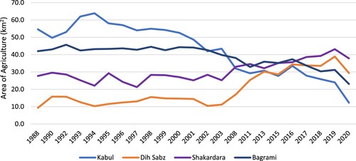
The agricultural area within each district for each year of the analysis is shown in Figure 4. The area of agriculture in the Kabul district reaches a max of 63.9 km² in 1994, then gradually declines to a minimum of 12.3 km² in 2020. Agricultural area in the Bagrami district also decreases across the 32 years of the study, from a maximum of 45.7 km² in 1992 to a minimum of 23.1 km² in 2018. Conversely, agricultural extent of the Dih Sabz district increases substantially from a minimum of 9.3 km² in 1988 to a maximum of 38.9 km² in 2019. In the Shakardara district agricultural area fluctuates around 27 km² from 1988 to 2003, before gradually increasing to a maximum of 43.2 km² in 2019. All 7 districts in the study area (including Kalakan, Mir Bacha Kot, and Shakardara) exhibited substantial decreases in agricultural area between 2019 and 2020.

Figure 4. Area of agriculture mapped within each district.

Line graph shows the area of agriculture (in square kilometers) by district for each year of analysis. The lines for the Kabul, Dih Sabz, Shakadara, and Bagrami districts indicate a range of areal extents that change over time – the Kabul and Bagrami lines both gradually decrease with time, and the Dih Sabz and Shakadara lines gradually increases with time.

The overall accuracy of the 2017 combined band ratio was found to be 87.1% with 75.5% and 84.3% producer’s and user’s accuracy (respectively) for agricultural area. Areas of obvious misclassification include the area immediately surrounding the airport runway and mountainous areas in the southwestern part of the study area.

3.2. Visualization of change results

The result of generalizing the combined band ratio result for each year to a 1 km² grid is shown in Figure 5 for the years 1988 and 2020; however, it should be noted that 24 individual maps were created of these results. In this figure, the expansion of agricultural area to the northeast of Kabul is visible in the emergence of dark green zones. The 1988 and 2020 maps were combined with the other 22 maps to create an animation of the changes in agricultural area over time (see attached files).

Figure 5. Results of combined band ratio analysis for 1988 (left) and 2020 (right).

Two map frames show the results of the combined band ratio analysis for 1988 (left frame) and 2020 (right frame) aggregated to the 1 square kilometer grid. While this aggregation appears coarse at the map scale in the two static maps, the animation of similar map frames for each year of analysis is more readily understandable than an animation of the original (non-aggregated) versions of the results.

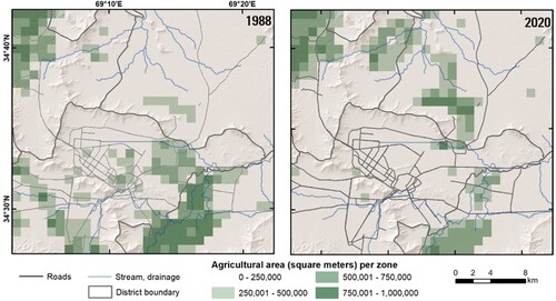
Conversely, to the southwest of the city of Kabul (but within the district of Kabul), the agricultural zones almost entirely disappear. In the Bagrami district to the southeast of the city, the green shade of the zones becomes lighter, indicating that there is approximately 25% less agricultural area in 2020 than in 1988.

Visualization of changes in agricultural land use over the past 32 years in one 2D map is shown in the map associated with this publication. The color legend for the map is shown using a matrix, where the rows indicate ranges of agricultural area (km²) and the columns indicate ranges of years. It is read from left to right, top to bottom, so that ‘The maximum extent of agriculture area in the gridcell was … . And occurred between the years of … .’ For example, the medium pink color that occurs around the Kabul city center indicates that the largest amount of agriculture that occurred in those gridcells was 0.2–0.5 km², and this extent occurred between 1988 and 2000. The extent of agricultural area in these gridcells during later dates was less than this amount. Conversely, the dark green cells that occur in the southwestern part of the Dih Sabz district indicate that a maximum area of 0.6–1.0 km² (up to 100% of the possible gridcell area) occurred in these gridcells, and this extent occurred between 2011 and 2020. Additionally, the key of the map shows the original color ramps assigned to the two attributes (area of maximum agriculture (in km²) and year of maximum agricultural extent) to provide the reader additional help in interpreting the map.

4. Discussion/conclusion

The extent of agricultural area is an important factor in assessing the food production capabilities of a region. This information is useful in the development of policies for land management, and is also sought by other government agencies. Remote-sensing based estimates of agricultural areas underestimate the extent of cultivation by not including fields that have been left fallow or just planted, yet this is a common and important practice in agronomy. By allowing fields to ‘rest’, absent of growing crops, the nutrient balance in the soil is restored, compaction is reduced, and aeration is improved. The integration of the Soil-Adjusted Vegetation Index (SAVI) with the ‘clay’ band ratio successfully highlighted areas of growing agricultural vegetation, as well as the fallow or just-planted fields. The 87.1% overall accuracy of the results suggests that this method is an accurate way to account for these oft-neglected areas of agricultural land use. The simplicity of this method is appealing because it can easily be applied to additional years of data without the need for extensive recalibration or estimation of complex variables. Moreover, all data and programming scripts used in this study have been provided to facilitate the reapplication of the results.

The success of the clay band ratio used in this study is interesting since the composition of surficial sediments in the broad flat lowlands of the Kabul basin is primarily wind-blown loess. The very-small size of these ultra-fine silt, sand, and clay particles that blanket the region, combined with the comparatively high soil moisture of agricultural fields is likely behind the success of the clay band ratio in this context. Very fine soil particles reflect higher percentages of most wavelengths compared to larger soil particles, so the fine wind-blown loam soil particles are highly reflective in VIS-SWIR wavelengths. However, the principal characteristic that differentiates cultivated fields from other areas of similar soil composition is the increased soil moisture of irrigated or plowed fields. While this increase in water enhances water absorption features in the SWIR wavelengths, it also diminishes the magnitude of the hydroxyl (clay) absorption feature that occurs near 2.2 μm. These two factors likely contribute to the success of the ‘clay’ band ratio in identifying fallow fields, a finding which is corroborated by DeWitt and others (2021). A further detailed explanation of this success would require spectral radiometer data and is beyond the scope of this analysis. Future work should also investigate the application of this combined band ratio method in other parts of Afghanistan, and other regions of the world.

The temporal detail of this study’s findings shows that substantial variability in the extent of agricultural land use occurs on an annual or semiannual basis in some districts (such as the Shakadara district), but in other districts (such as the Bagrami district) the extent of agricultural land use stayed relatively consistent for large parts of the study. The long period of study duration (24 observations covering 32 years) also allows for the identification of long-term trends in shifting land use between districts. This shift is most apparent in the Kabul district, which experienced substantial decrease in cultivated land over time, and the Dih Sabz district, which experienced a substantial increase in cultivated land over time. The decrease in agricultural extent across all districts in 2020 is also noteworthy. 

4.1. Visualization

In temporal change analyses, the inclusion of the 4th dimension via multiple ‘time stamp’ maps greatly increases the volume of information conveyed by the map(s), which necessitates generalization of results to a level appropriate for the number of time stamps included in the visualization. Essentially this ‘multi-map’ display of change results requires the audience to not only remember, but to mentally compare the map frame currently in view with previously viewed frames. This is not difficult when the frames lie next to each other (Figure 3 and Figure 5) – the maps individually are not difficult to understand, and the detailed results shown in Figure 3 are generally preferable. However, when 24 maps are viewed together side by side the map comparison becomes much more difficult. In animated form, the previous ‘time stamps’ are not simultaneously visible, and the rapidity with which the results of each map must be ingested and mentally compared by the viewer means that a simpler generalized map more effectively conveys the information. Thus, in animated form, the maps shown in Figure 5 (used to create animation 2) are generally preferable to those in Figure 3 (used to create animation 1).

While animations provide an excellent medium to convey the results of time series analysis, a single two-dimensional map is still arguably the most effective way to preserve and convey geographic information because it transcends technological changes. Thirty-two years of agricultural change were condensed into a single map by synthesizing the results down into two key concepts: the maximum agricultural extent found in each gridcell over the 32 years of analysis, and the year in which that maximum extent occurred in each gridcell. Despite the conceptual simplicity, a large volume of information is still conveyed by this 2D map product. In essence, all of the 24 frames from the zonal mapping animation are condensed down into each factor. Integration of both themes into one map requires the audience two interpret two separate color ramps and their 9 potential combined colors. This information content is visually displayed as a matrix legend, which is complex, but still the most efficient and effective way to convey mapped information.

4.2. Implications for agricultural change in Kabul

The landscape of Kabul, Afghanistan has changed substantially over the 32 years of this study. While this has been somewhat documented by other studies and reports, this report publishes the longest and most detailed analysis (24 years of analysis covering a span of 32 years between 1988 and 2020 at 30 m resolution) available of agricultural extent in the greater Kabul area. While some of the observed trends are expected, others are unanticipated. The decrease in agricultural extent in the Kabul district is a natural consequence of the expansion of development and peri-urban spaces as the city of Kabul becomes a sprawling urban center. The expanding population of this sprawling urban center still requires the foodstuffs grown in the immediate vicinity, thus it is not unexpected that the agricultural area has not disappeared, but rather shifted to other areas.

However, the substantial increase of agricultural land use in the Dih Sabz district is somewhat unexpected because of its aridity and distance from the primary drainage arteries (namely, the Kabul River). There are significant implications of this shift for planning and management to consider. In particular, the sustainability of water usage for expanding agricultural activity in an arid region should be carefully considered. Where run-off fed water supply is insufficient, there is a heavy reliance on water pumped from near-surface aquifers. These aquifers have traditionally supplied most of the drinking water for the Kabul region. With increased aquifer-based irrigation, shallow wells will run dry or need to be extended into deeper layers of the aquifer. The implications of climate change and increased variability of precipitation may also be important to the long-term sustainability of agriculture in Dih Sabz.

Finally, the substantial decrease in agricultural extent across all districts between 2019 and 2020 is an interesting change from the long-term trend of most areas. Additional observations in subsequent years will be necessary to determine if this decrease becomes a more enduring trend.

Software

Band ratio analyses and zonal statistics operations were conducted using PyCharm. Microsoft Excel was used to assess agricultural area and other statistical values over time, as well as to create graph figures. ESRI ArcMap was used to do all other geospatial analysis and map development. Map layout was further edited using Adobe Illustrator.

Acknowledgements

The authors would like to recognize Thomas Mack (internal reviewer USGS) for valuable comments on an early version of the manuscript; Robert Stamm (USGS) for valuable review and copy editing of the manuscript and data release.

Disclosure statement

No potential conflict of interest was reported by the author(s).

Data availability statement

The Landsat imagery used in this study is freely available and can be downloaded from the USGS Earth Explorer (https://earthexplorer.usgs.gov). Other files, including the band ratio analysis results for each year and the urban land cover data are available at Sciencebase.gov under https://doi.org/10.5066/P9IC4QFW.

Additional information

Funding

This work was supported by United States Agency for International Development [grant number 72030618T00002].

References

- Boettinger, J. L., Ramsey, R. D., Bodily, J. M., Cole, N. J., Kienast-Brown, S., Nield, S. J., Saunders, A. M., & Stum, A. K. (2008). Chapter 16, Landsat spectral data for digital soil mapping. In A. E. Hartemink (Ed.), Digital soil mapping with limited data (pp. 193–202). Springer.
- Broshears, R. E., Akbari, M. A., Chornack, M. P., Mueller, D. K., & Ruddy, B. C. (2005). Inventory of ground-water resources in the Kabul Basin, Afghanistan, U.S. Geological Survey Scientific Investigations Report 2005-5090.
- Chang, J., Hansen, M., Pittman, K., Carrol, M., & DiMiceli, C. (2007). Corn and soybean mapping in the United States using MODIS time-series data sets. Agronomy Journal, 99(6), 1654–1664. https://doi.org/10.2134/agronj2007.0170
- DeWitt, J. D., Chirico, P. G., Alessi, M. A., & Boston, K. M. (2021). Remote sensing inventory and geospatial analysis of brick kilns and clay mining in Kabul, Afghanistan. Minerals, 11(3), 296–317. https://doi.org/10.3390/min11030296
- FAO. (2018). 15 Years in Afghanistan a special report: 2003-2018. Rome. 126 pp. http://www.fao.org/3/CA14336EN/ca1433en.pdf.
- Ghulami, M. (2017). Assessment of climate change impacts on water resources and agriculture in data-scarce Kabul basin, Afghanistan, HAL archives-ouvertes, Université Côte d’Azur; Asian institute of technology. HAL Id: tel-01737052, https://tel.archives-ouvertes.fr/tel-01737052
- Haboudane, D, Miller, J, Tremblay, N, Zarco-Tejada, P, & Dextraze, L. (2002). Integrated narrow-band vegetation indices for prediction of crop chlorophyll content for application to precision agriculture. Remote Sensing of Environment, 81(2-3), 416–426. https://doi.org/10.1016/S0034-4257(02)00018-4
- Hawbaker, T., Vanderhoof, M., Beal, Y., Takacs, J., Schmidt, G., Falgout, J., Williams, B., Fairaux, N., Caldwell, M., Picotte, J., Howard, S., Stitt, S., & Dwyer, J. (2017). Mapping burned areas using dense time-series of Landsat data. Remote Sensing of Environment, 198, 504–522. https://doi.org/10.1016/j.rse.2017.06.027
- Huang, C., Wylie, B., Yang, L., Homer, C., & Zylstra, G. (2002). Derivation of a tasseled cap transformation based on Landsat 7 at-satellite reflectance. International Journal of Remote Sensing, 23(8), 1741–1748. https://doi.org/10.1080/01431160110106113
- Huete, A. R. (1988). A soil-adjusted vegetation index (SAVI). Remote Sensing of Environment, 25(3), 295–309. https://doi.org/10.1016/0034-4257(88)90106-X
- Jensen, J. R. (2007). Remote sensing of the environment, an earth resource perspective. Pearson Prentice Hall. 592 p.
- Jones, R., Narayan, T., & Conrad, A. (2019). Mid-term performance evaluation of the regional agriculture development program in Afghanistan, estimating percentage change in land area under licit agriculture in program areas. USAID report. Accessed online at https://pdf.usaid.gov/pdf_docs/PA00TK15.pdf
- Kawasaki, S., Watanabe, F., Suzuki, S., Nishimaki, R., & Takahashi, S. (2012). Current situation and issues on agriculture of Afghanistan. Journal of Arid Land Studies, 22(1), 345–348.
- Khaliq, A. J. A., & Boz, I. (2018). The Role of agriculture in the economy of Afghanistan, 2nd International Conference on Food and Agriculture Economics, April 2018, Alanya, Turkey.
- Mack, T. J., Chornack, M. P., & Verstraeten, I. M. (2014). Sustainability of water supply at military installations, Kabul Basin, Afghanistan, in Igor Linkov, ed., Sustainable cities and military installations: Northern Atlantic Treaty Organization Science for Peace and Security Series C: Environmental Security, http://doi.org/10.1007/978-94-007-7161-1_11
- Maletta, H. E. (2007). Food and agriculture in Afghanistan: A long term outlook. In A. Palmisano & G. Ricco (Eds.), Afghanistan – how much of the past in the new future (pp. 10). ISIG. Available at SSRN: https://ssrn.com/abstract = 644301.
- Najmuddin, O., Deng, X., & Bhattacharya, R. (2018). The dynamics of land Use/cover and the statistical assessment of cropland change drivers in the Kabul River Basin, Afghanistan. Sustainability, 10(2), 423. https://doi.org/10.3390/su10020423
- Ott, T., & Swiaczny, F. (2001). Time-Integrative geographic information systems. Springer. 248 p., https://doi.org/10.1007/978-3-642-56747-6.
- Pain, A., & Shah, S. M. (2009). Policymaking in agriculture and rural development in Afghanistan, Afghanistan Research and Evaluation Unit, Case Study Series, Paul McCann and Mia Bonarski ed., 64p.
- Pan, Z., Huang, J., Zhou, Q., Wang, L., Cheng, Y., Zhang, H., Blackburn, G. A., Yan, J., & Liu, J. (2015). Mapping crop phenology using NDVI time-series derived from HJ-1 A/B data. International Journal of Applied Earth Observation and Geoinformation, 34, 188–197. https://doi.org/10.1016/j.jag.2014.08.011
- Pătru-Stupariu, I., Stupariu, M., Cuculici, R., & Huzui, A. (2011). Understanding landscape change using historical maps. Case study Sinaia, Romania. Journal of Maps, 7(1), 206–220. https://doi.org/10.4113/jom.2011.1151
- Pervez, M. S., Budde, M., & Rowland, J. (2014). Mapping irrigated areas in Afghanistan over the past decade using MODIS NDVI. Remote Sensing of Environment, 149, 155–165. https://doi.org/10.1016/j.rse.2014.04.008
- Safi, Z., Dossa, L. H., & Buerkert, A. (2011). Economic analysis of cereal, vegetable and grape production systems in urban and peri-urban agriculture of Kabul, Afghanistan. Experimental Agriculture, 47(4), 705–716. https://doi.org/10.1017/S0014479711000482
- Taher, M. R., Chornack, M. P., & Mack, T. J. (2014). Groundwater levels in the Kabul Basin, Afghanistan, 2004–2013: U.S. Geological Survey Open-File Report 2013–1296, 51 p., http://doi.org/10.3133/ofr20131296
- The World Factbook. (2020). Washington, DC: Central Intelligence Agency, 2020, https://www.cia.gov/the-world-factbook/ on 1/25/2021
- Tiwari, V., Matin, M. A., Qamer, F. M., Ellenburg, W. L., Bajracharya, B., Vadrevu, K., Rushi, B. R., & Yusafi, W.. (2020). Wheat area mapping in Afghanistan based on optical and SAR time-series images in google earth engine cloud environment. Frontiers in Environmental Science, 8(77), 15. https://doi.org/10.3389/fenvs.2020.00077
- Tünnermeier, T., & Houben, G. (2005). Hydrogeology of the Kabul Basin Part I: Geology, aquifer characteristics, climate and hydrography, Federal Institute for Geoscience and Natural Resources (BGR), record no. 10277/05, Hannover, Germany.
- United Nations. (2018). World Urbanization Prospects: The 2018 Revision, Online Edition, Department of Economic and Social Affairs, Population Division, https://population.un.org/wup/Download/