Estimation of rainfall-induced surface runoff for the Assam region, India, using the GIS-based NRCS-CN method

ABSTRACT

The NRCS-CN method, integrated with GIS and remote sensing, can be used for estimating curve numbers (CN) and surface runoff in geohydrological systems. The study area is divided into 63 sub-basins, and the land use land cover (LULC)-hydrologic soil group (HSG) complex is identified for each sub-basin. The CN values for three antecedent soil moisture (AMC) conditions are calculated and corrected for surface slope variations. The surface runoff depth is determined using the rainfall data for 16 years (2005–2020). The average runoff depth and mean annual precipitation ranges from 444.50 to 1960.55 mm and 936.99 to 3520.55 mm, respectively. For all sub-basins, strong correlations between runoff depth and rainfall (R² ≥ 0.8) as well as between simulated runoff and measured runoff (R² ≥ 0.8) are observed. The Nash–Sutcliffe model efficiency coefficient (NSE) values suggest that the model's efficiency is good to satisfactory.

KEYWORDS:

• Curve number
• NRCS-CN method
• runoff depth
• Assam
• GIS

1. Introduction

With increased urban sprawling and changes in land-use patterns, the available water resources on the earth are experiencing excessive pressure (Bera et al., 2021; Satya et al., 2020). The threat of urban flooding is also arising due to increased impervious land, a higher ratio of rainfall to infiltration rate, and a lower groundwater recharge rate (Devi et al., 2019; Mukherjee et al., 2018; Pathak et al., 2020). The branch of hydrology plays a significant role in effective water resource management of an area by quantifying and assessing the relationship between the amount of precipitation, catchment area, length of the dry period, storage capacity, amount of runoff, evaporation, and transpiration (Psomiadis et al., 2020; Tian et al., 2020). Floods and other natural hazards affect the socio-economic scenario of a region (Agrawal et al., 2021). Accurate estimation of rainfall-induced surface runoff is essential for water resource management and flood control measures (Abdessamed & Abderrazak, 2019).

Runoff is the significant portion of the precipitation transferred as flow to the streams or nearby waterways after being captured by the terrestrial soil and vegetation (Kumari et al., 2019). It mainly occurs when the precipitation rate exceeds the infiltration rate and depends on rainfall intensity, slope, soil texture, catchment area, LULC, etc. (Garg et al., 2013; Kumar, 2021; Rao, 2020; Saran et al., 2021). The National Resources Conservation Service-Curve Number (NRCS-CN) method, developed by the NRCS, United States Department of Agriculture (USDA) in 1976, is used frequently for estimating surface runoff (Akbari et al., 2021; Farran et al., 2021).

It is based on the basic empirical formula and estimates rainfall-runoff relationships by obtaining curve number maps, so detailed information regarding the spatial distribution of LULC, and soil profile are required (Ajmal et al., 2016; Deshmukh et al., 2013; Ebrahimian et al., 2012; Zhang, 2019). Remote sensing (RS) and geographical information systems (GIS) act as efficient and powerful tools for hydrogeomorphological modeling (Gupta et al., 2021; Patil et al., 2008; Verma et al., 2017). The application of GIS has enabled the use digital elevation model for hydrological modeling based on the topography of a region. RS helps to extract the topography, LULC, soil profile, drainage characteristics, etc., of a region that can be stored as a geo-referenced database in GIS. The extracted layers are then combined with meteorological parameters in the GIS environment to analyze further, interpret, and visualize to develop rainfall-runoff models (Ebrahimian et al., 2009; Mohammad & Adamowski, 2015; Rajbanshi, 2016). Using traditional methods to calculate runoff from a given watershed, especially for inaccessible terrain, is time-consuming and complex due to the spatiotemporal variability of hydrological parameters, but the application of geospatial datasets has made it reliable, flexible, and accepted by researchers, hydrologists, and planners (Ajmal et al., 2016; Bal et al., 2021; Lian et al., 2020).

Many researchers have estimated GIS-based surface runoff using the NRCS-CN method (Al-Ghobari et al., 2020; Kumar et al., 2016; Rao, 2020; Tirkey et al., 2014; Verma et al., 2017). Satheeshkumar et al. (2017) analyzed the efficiency of GIS-based runoff estimation for the Pappiredipatti watershed using the NRCS–CN model for different AMCs. Rawat and Singh (2017) observed that rainfall and runoff, estimated by the NRCS-CN method using LANDSAT-7ETM+, NOAA data for the Jhagrabaria watershed in Allahabad district, are strongly correlated. Pathan and Joshi (2019) estimated runoff of the Karjan reservoir basin in the Narmada district by the GIS-based NRCS-CN method and found a strong correlation between measured and simulated runoff. Kumar (2021) performed the runoff estimation for the Sind river basin by integrating the NRCS-CN method with GIS and concluded that the technique is efficient for large datasets and broader environmental sites.

The present study aims to develop a GIS-based rainfall-induced Srunoff model for the Assam region, India, using the NRCS-CN method. Floodplains of the Brahmaputra river mainly cover the Assam region, and it is highly flood-prone during the monsoon. It provides a decision-making support system for implementing effective and sustainable water resource management and flood mitigation measures for the flood risk zones.

2. Material and methods

2.1. Study area

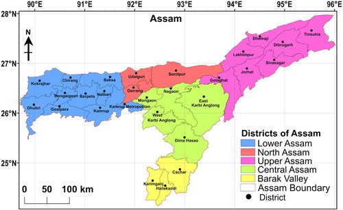
Assam region is situated in the north-east of India (24° 8′ N to 28° 2′ N latitude and 89° 42′ E to 96° E longitude), covering approximately 78,438 km², with an elevation of 45–1964 m above the mean sea level. It is mainly divided into five administrative divisions, i.e. Barak valley, Lower, Northern, Upper, and Central Assam (Figure 1). This region is prone to multiple natural hazards (Dixit et al., 2016; Raghukanth et al., 2011). The climate is tropical monsoon rainforest with heavy rainfall and high humidity (Garaga et al., 2020; Gupta & Dixit, 2022). The temperature in summers ranges from 32°C to 38°C and in winters from 8°C to 20°C. The region experiences heavy rain due to the southwest monsoon, mainly from May to September, and the annual rainfall ranges between 1500–3750 mm (Sharma et al., 2020). The population primarily depends on agriculture as their source of income, and the population growth rate is about 16.93% (Census, 2011).

Figure 1. Map of the study area.

This figure illustrates a map of the study area showing the location of Assam state, located in the north-eastern part of India. It also illustrates the five administrative divisions of Assam along with the name of the 27 districts.

Due to heavy monsoon and the Brahmaputra river, the Assam region experiences floods every year, lakhs of people become homeless, and damages to agricultural lands and crops occur. (Kumar, 2021; Pal & Singh, 2018).

2.2. Dataset used

In the present study, elevation, LULC, rainfall, etc., datasets are obtained from different sources, and details of the dataset are provided in (Supplementary Table S1).

2.3. National Resources Conservation Services-Curve Number (NRCS-CN) method

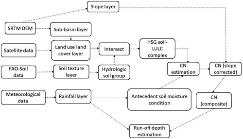
The NRCS-CN method estimates direct runoff using a simple empirical equation based on the rainfall, soil, LULC, and the curve number (CN) (Figure 2) (Mishra et al., 2018; NRCS, 2004; USDA, 1985). The HSG-LULC complex and antecedent soil moisture (AMC) determines the curve number (Ebrahimian et al., 2009; Mohammad & Adamowski, 2015). In the NRCS-CN method, the ratio of actual retention (F) to the potential maximum retention (S) is equal to the ratio of direct runoff (Q) to rainfall (P) minus initial abstraction (I) as given by equation (1) (1) ${\displaystyle \frac{F}{S}={\displaystyle \frac{Q}{(P-I)}}}$(1)

Figure 2. Methodology for the estimation of surface runoff.

This figure represents the overall methodology applied in the study. It shows the different layers and their source, and the steps required to estimate surface runoff.

Here, the unit of F, S, P, Q, and I are in mm.

Actual retention, F, can be given by the equation (2) (2) $F=P-I-Q$(2)

Combining equation (1) and equation (2), Q can be defined as shown in equation (3) (3) $Q={\displaystyle \frac{{(P-I)}^2}{(P-I+S)}}$(3)

The relation between initial abstraction (I) and potential maximum retention (S) is shown by equation (4), where λ is the initial abstraction coefficient varying from 0 to infinity, for the general use value of 0.2 is recommended. (4) $I=\lambda S$(4)

The value of Q can be expressed for two different conditions of P as given by equation (5) and equation (6).

For P > λS. (5) $Q={\displaystyle \frac{{(P-\lambda S)}^2}{P+(1-\lambda )S}}$(5) (6) $\mathrm{For}P\le \lambda SQ=0$(6)

I is a function of S, and replacing I with 0.2S, equation (7) is obtained. (7) $Q={\displaystyle \frac{{(P-0.2S)}^2}{P+0.8S}}$(7)

The relation between potential maximum retention S and Curve Number CN can be represented as (Pathak et al., 2020; Tirkey et al., 2014): (8) $S=254({\displaystyle \frac{100}{CN}-1)}$(8) where CN is a dimensionless parameter ranging between 0–100, the potential maximum retention S can vary between 0-ꝏ, and the constant 254 represents S in mm. Equation (8) establishes the relationship between S and CN to show the linear trend of the operations like averaging, weighting, and interpolation (NRCS, 2004).

Three levels of AMC are used: AMC-I, AMC-II, and AMC-III for dry, normal, and wet conditions, respectively (NRCS, 2004).

The CNII is further converted to CNI and CNIII for AMC-I and AMC-III, respectively, by equations (9) and (10). (9) $\begin{array}{rl}& CNI={\displaystyle \frac{4.2\times CNII}{10-(0.058\times CNII)}}\\ & \end{array}$(9) (10) $CNIII={\displaystyle \frac{23\times CNII}{10+(0.013\times CNII)}}$(10)

Each basin consists of a different LULC-HSG complex, so CN values are determined for each complex, and finally, the composite curve number (CN_w) is estimated by weighting the resulting CN values by using the equation (11) (11) $C{N}_W={\displaystyle \frac{\sum C{N}_i\times A_i}{A}}$(11) where CN_i is the curve number of the sub-region, A_i represents the sub-basin area with the associated curve number, and A represents the total study area.

The slope is a significant factor in determining runoff and CN, so it is essential to incorporate slope-corrected CN values (Garg et al., 2013). In the present study, the CN values are adjusted to include the slope factor using equation (12) given by Huang et al. (2006) (12) $CNI{I}_{\alpha }={\displaystyle \frac{(CNIII-CNII)}{3}(1-2e^{-13.86\alpha })+CNII}$(12)

CNII_α signifies slope-corrected CNII for normal conditions, and α is the average slope of the basin.

2.4. Delineation of sub-basins and extraction of streams using DEM data

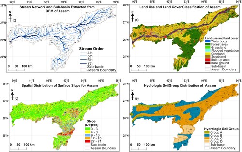
The elevation profile of the study area is generated from the SRTM Digital Elevation Model (DEM) of 1 arc-second (30 m resolution) stream network, and 63 sub-basin layers are extracted from it using GIS hydrology tools (Figure 3a) (Taesiri et al., 2020). The vertical accuracy of SRTM DEM 30 m is more accurate, and it has a better quality to extract slope and drainage network (Rawat et al., 2019).

Figure 3. (a) Sub-basin with stream network, (b) Land use and land cover, (c) Surface slope, and (d) Hydrologic soil group.

This figure illustrates the different layers required to estimate curve number (CN). Long Description: This figure illustrates the different layers required to estimate curve number (CN). In this figure (a) shows 63 delineated sub-basins of the study area with different stream orders ranging from 4 to 7, figure (b) represents eight classes of land use land cover, figure (c) shows the spatial variation of the slope of the study area, and in figure (d) Hydrologic soil group map of the study area is given, and it is derived from the soil texture map.

2.5. Accuracy assessment of LULC

The LULC map for the study area is derived from Sentinel-2 imagery (10 m resolution) and classified into eight classes (Karra et al., 2021). With the help of Google Earth satellite images, the accuracy of the LULC map is analyzed by determining overall accuracy (OA) and Kappa (K) statistics using a detailed error matrix for each classified image (Hishe et al., 2020; Vignesh et al., 2021) using equations (13) and (14), respectively. OA mainly considers the relative weight of each class and is calculated by dividing the total number of accurately classified pixels by the total number of pixels taken into consideration (Verma et al., 2017). (13) $OA=\left({\displaystyle \frac{\sum _{i=1}^n{M}_{ii}}{\sum _{i=1}^n\sum _{j=1}^n{M}_{ij}}}\right)\times 100\text{\%}$(13) where n represents the number of classes, M_ii represents the number of sample points in row i and column i of the matrix, and M_ij are row i and column j elements.

The range of the Kappa coefficient lies between 0–1, and the higher coefficient value denotes higher accuracy (Rwanga & Ndambuki, 2017). It is mainly applied to assess the random classification results and accuracy of remote sensing imagery (Talukdar et al., 2020). (14) $K={\displaystyle \frac{N\sum _{i=1}^r{M}_{ii}-\sum _{i=1}^r(M_{i+})(M_{+i})}{N^2-\sum _{i=1}^r(M_{i+})(M_{+i})}}$(14)

N denotes total sample points, M_ii represents the number of sample points on the diagonal of the matrix, M_+i and M_i+ are the number of samples of each row (r) and column (i), respectively.

For each LULC class, the User’s accuracy (UA) and Producer’s accuracy (PA) are also calculated using equations (15) and (16) (15) $UA={\displaystyle \frac{Nii}{Nirow}\times 1000/0}$(15) (16) $PA={\displaystyle \frac{Nii}{Nicolumn}\times 1000/0}$(16)

N_ii represents the number of samples of each class correctly matched in the i^th row and column, N_irow equals the total number of samples in the i^th row, and N_icolumn represents the total number of samples in the i^th column.

2.6. Determination of correlation between rainfall and runoff depth

To estimate the correlation between rainfall (P) and runoff depth (R), linear regression is performed for 63 sub-basins using the equation given by Subramanya (2006) shown in equation (17). The coefficient of determination (r) of each sub-basin is obtained from equation (18) (17) $R=mP+n$(17) (18) $r={\displaystyle \frac{N(\mathrm{\Sigma }PR)-(\mathrm{\Sigma }P)(\mathrm{\Sigma }R)}{\sqrt{[N(\mathrm{\Sigma }{P}^2)-{(\mathrm{\Sigma }P)}^2][N(\mathrm{\Sigma }{R}^2)-{(\mathrm{\Sigma }R)}^2]}}}$(18)

N denotes the number of observations, n is the intercept, and m is the slope of the linear regression straight line.

2.7. Determination of correlation between simulated and measured runoff depth

Generally, the actual runoff is calculated by the field measurement following a rainfall event. In the present study, since the conventional hydrological data were not available for all the sub-basins, so the measured runoff of each sub-basins is calculated with the help of the regression equation (19) by considering N number of observations of runoff determined by NRCS-CN (R) and rainfall (P) as input parameters (Chanu et al., 2015; Kumar et al., 2016). The constant x and y can be calculated using equations (20) and (21). (19) $\mathrm{Measured}\mathrm{runoff}=x+(y\times \mathrm{rainfall})$(19) (20) $y={\displaystyle \frac{N(\mathrm{\Sigma }PR)-(\mathrm{\Sigma }P)(\mathrm{\Sigma }R)}{N(\mathrm{\Sigma }{P}^2)-{(\mathrm{\Sigma }P)}^2}}$(20) (21) $x={\displaystyle \frac{\mathrm{\Sigma }R-y\mathrm{\Sigma }P}{N}}$(21)

2.8. Performance evaluation of the method

Performance evaluation of the method used in the present study is conducted to determine the goodness of fit between the simulated and measured values (Ritter & Munoz-Carpena, 2013). To evaluate the accuracy of the method, Nash–Sutcliffe model efficiency coefficient (NSE) values are determined as given by equation (22) (Chanu et al., 2015; Deshmukh et al., 2013; Nash & Sutcliffe, 1970; Zhang, 2019) (22) $NSE=\left(1-{\displaystyle \frac{\mathrm{\Sigma }{(Qmsd-Qsim)}^2}{\mathrm{\Sigma }{(Qmsd-Qmean)}^2}}\right)\times 100$(22)

Here, Q_msd, Q_sim, and Q_mean denote the measured, simulated, and mean of the measured runoff depth in mm. If the value of NSE is 100%, it indicates that a perfect agreement exists between measured and simulated values. The NSE will become zero for the equal measured and simulated runoff depth value.

3. Results

3.1. LULC map and its accuracy assessment

The LULC map is classified into eight classes, and its accuracy is validated by the overall accuracy assessment and Kappa coefficient determination method. A total of 884 sampling points are taken and validated by Google Earth images. The value of overall accuracy and Kappa coefficient are 89.81% and 0.87, respectively. The User’s and Producer’s accuracy for each LULC class is greater than 80% (Table 1) (Zhou et al., 2018).

Table 1. Accuracy assessment of LULC map.

LULC Class	WB	FA	GL	FV	CL	SL	BLT	BL	Total User	UA (%)
WB	97	0	3	0	0	0	0	3	103	94.17
FA	0	100	8	0	0	2	0	0	110	90.91
GL	1	5	103	2	3	4	0	1	119	86.55
FV	2	0	2	94	4	2	0	1	105	89.52
CL	0	2	3	2	102	3	0	3	115	88.70
SL	2	0	3	0	2	99	0	8	114	86.84
BLT	0	0	0	0	4	0	98	2	104	94.23
BL	3	0	0	0	3	4	3	101	114	88.60
Total Producer	105	107	122	98	118	114	101	119	884
PA (%)	92.38	93.46	84.43	95.92	86.44	86.84	97.03	84.87

WB- Water body; FA- Forest area; GL- Grassland; FV- Flooded Vegetation; CL- Cropland; SL- Scrubland; BLT- Built-up area; BL- Barren land; UA- User’s Accuracy; PA- Producer’s Accuracy

According to the LULC map, most of the study area is covered by forest and agricultural land (Figure 3b). Forest areas are predominant in Central Assam, the hilly region, whereas agricultural lands are dominant around the flood plains of the Brahmaputra river and Barak river basin extending from Lower to Upper Assam. A high built-up area density is observed in Lower, Northern, And Upper Assam. The areas with low vegetation cover like the urban, barren land, and scrubland have higher runoff volumes and show a good correlation between rainfall and runoff. Similar results were shown by Bal et al. (2021), Koneti et al. (2018), and Mukherjee et al. (2018), where a strong correlation between vegetation cover and runoff depth is observed.

3.2. Variation of surface slope

In the present study, the slope map is derived from SRTM DEM (30 m resolution) and classified into five classes nearly flat (0°−3°), gentle (4°−8°), moderate (9°−16°), steep (17°−26°), and very steep (27°−71°) (Figure 3c). Most of the study region is nearly flat, and moderate to very steep slope classes are observed in Central Assam.

3.3. Hydrologic soil group (HSG)

The HSG map is classified into four classes of HSG, i.e. A, B, C, and D (Figure 3d). According to NRCS US (2009), the four groups of HSG differ in texture, water transmission rate, and infiltration capacity as (i) Group A (sand, loamy sand, or sandy loam soil) has low runoff potential, high infiltration rates, and high water transmission rate. (ii) Group B (silt loam or loam soil) is characterized by having a moderate infiltration rate (iii) Group C (sandy clay loam soil) with moderately fine to fine texture has a low infiltration rate. (iv) Group D (clay loam, silty clay loam, sandy clay, silty clay, or clay) are clay soils with the highest runoff potential and very low infiltration rates.

The Brahmaputra basin is predominantly covered by HSG C, and the Barak river basin is dominated by HSG D. In some parts of Lower, Central, and Barak valley HSG B (loam) is present. HSG A is mainly present in the upper part of Lower Assam and has the highest infiltration rate (NRCS, 2009). Due to the dominance of HSG C and HSG D, the study region have a slow transmission rate and infiltration rate; as a result, it can contribute to a large amount of surface runoff during a rainfall event (Al-Ghobari et al., 2020). Therefore, the sub-basins with HSG C and HSG D will have higher runoff depth.

3.4. Estimation of curve number (CN)

In the present study, the CN values of each sub-basin are determined by intersecting the LULC and HSG layers. The CNI, CNII, and CNIII values are determined for all corresponding AMCs, i.e. AMC-I, AMC-II, and AMC-III conditions (Table 2). The CNI values for Lower and Upper Assam fall from 52 to 67, for Northern and Central Assam from 42 to 51, and for Barak valley from 48 to 56 (Figure 4a). The CNII values vary between 72–83 for Lower and Upper Assam, 68–74 for Barak valley, and 63–71 for Northern and Central Assam (Figure 4b). In CNIII, the values lie between 86–93 for Lower and Upper Assam, 83–87 for Barak valley, and 80–85 for Northern and Central Assam (Figure 4c).

Figure 4. Spatial distribution of (a) Curve number I, (b) Curve number II, (c) Curve number III, (d) Slope-corrected curve number I, (e) Slope-corrected curve number II, and (f) Slope-corrected curve number III.

This figure represents the calculated value of curve number (CN) for the different sub-basins of the study area. Long Description: This figure represents the calculated value of curve number (CN) for the different sub-basins of the study area. In this figure (a) shows CNI for AMCI, figure (b) shows the CNII value for AMC II, and figure (c) describes CNIII for AMC III. The three Curve numbers are then corrected according to the slope and given in figure (d) as slope-corrected CNI, figure (e) as slope-corrected CNII, and figure (f) as slope-corrected CNIII.

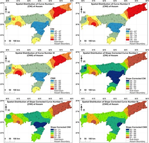
Table 2. Estimation of curve number for each LULC-HSG complex of the study area.

Land use land cover (LULC)	Hydrologic soil group (HSG)	Area (km^2)	Curve number (CN)	CN*Area	WCN
Waterbody	A	225.39	98	22088.09	AMC-II-76.37
	B	676.16	98	66263.30	AMC-I-57.58
	C	2408.30	98	236013.43	AMC-III-88.14
	D	128.16	98	12559.68
Forest area	A	1406.89	45	63310.05
	B	12240.90	53	648767.67
	C	11576.73	67	775641.19
	D	5157.67	72	371352.24
Grassland	A	68.66	61	4188.36
	B	163.81	77	12613.39
	C	403.62	85	34307.65
	D	21.83	91	1986.53
Flooded vegetation	A	1.40	77	107.63
	B	78.95	80	6316.12
	C	145.29	83	12059.28
	D	8.12	86	698.14
Cropland	A	1077.33	62	66794.66
	B	8208.76	71	582821.78
	C	15899.17	88	1399126.66
	D	1558.74	91	141845.34
Scrubland	A	307.79	63	19390.85
	B	657.92	77	50660.18
	C	1898.91	85	161407.66
	D	167.77	88	14763.76
Built-up area	A	368.93	89	32835.04
	B	3399.64	92	312767.22
	C	5959.50	94	560193.06
	D	600.35	95	57033.25
Barren land	A	379.02	77	29184.27
	B	334.59	86	28774.43
	C	2905.46	91	264397.27
	D	2.64	94	248.16
	Total	78438.41		5990516.34

Higher values of CNs are observed for Upper, and Lower Assam, moderate to low CN values are found in Barak valley, and very low to low CN values for the Northern and Central Assam region. The spatial distribution of CNs indicates that areas with a higher value of CN, like Lower Assam, represent the presence of impervious areas with little vegetation cover along with high built-up area, and areas having low to moderate CNs values like Barak valley will exhibit lower runoff due to dense vegetation cover in the form of forest area (Al-Ghobari et al., 2020; Kumar et al., 2016).

Shi and Wang (2020) and Huang et al. (2006) highlighted the significance of slope corrected curve number, the surface runoff generation increases with a steeper slope. So, the CNI, CNII, and CNIII values are further corrected according to the surface slope variation of the study area (Garg et al., 2013; Huang et al., 2006; Shi & Wang, 2020). The slope corrected CNI, CNII, and CNIII are estimated between 48-72, 69-86, and 83-93, respectively, which slightly varies from the slope uncorrected curve numbers (Figure 4d-f). Due to the small area falling under the steep slope class, LULC and HSG exceeded the effect of the slope factor and thus causing only a slight variation of the spatial distribution of curve number in the study area. In the case of Central Assam and Barak valley, the slope corrected curve numbers are less than floodplains because of high vegetation density.

3.5. Rainfall data

The spatial distribution of the mean annual precipitation (MAP) is estimated using the inverse distance weighting (IDW) interpolation method (Caloiero et al., 2020; Al-Ghobari et al., 2020). MAP ranges between 1552-3520 mm for Lower, and Upper Assam, 1956 - 3520 mm for Barak valley, 1552 −1955mm for Northern Assam, and 936-1551 mm is observed for the Central Assam region (Figure 5a). The daily rainfall data is further analyzed to determine the AMC condition to estimate CN values associated with AMC, initial abstraction for each year, and corresponding maximum retention value (Farran & Elfeki, 2020; Karunanidhi et al., 2020; Sanz-Ramos et al., 2020).

Figure 5. (a) Mean annual precipitation and (b) Surface runoff depth.

This figure consists of figure (a) Mean annual precipitation map for the study area and 5(b) Surface runoff depth map for the study area. Long Description: This figure consists of two figures, Figure (a) represents the mean annual precipitation for the study area derived from 16 years of rainfall data, and the unit is given in mm. Figure (b) shows the surface runoff depth map for the study area, estimated from the rainfall data and Curve number values (CN).

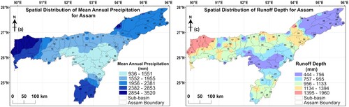
3.6. Estimation of surface runoff

The runoff depth ranges from 444 mm to 1724mm (Figure 5b). In the Lower Assam, most of the site shows moderate to very high runoff depth ranging between 956-1724mm due to high built-up area, high CN, high precipitation, and less vegetation cover. For the Northern and Upper Assam, the runoff depth falls in 444-1394 mm, a very low to high range. In the case of Central Assam, due to dense vegetation cover, low precipitation, and lower value of CN, the estimated runoff depth lies in very low to low class, i.e. 444-955 mm. Areas with high rainfall, less vegetation cover, and impervious soil profiles are experiencing high surface runoff due to decreased infiltration rate and water abstraction (Deshmukh et al., 2013). More runoff depth is generated on steep slopes than on flat plains due to increased slope angle, the infiltration rate, initial abstraction, and recession period decrease (Ajmal et al., 2016; Ebrahimian et al., 2012).

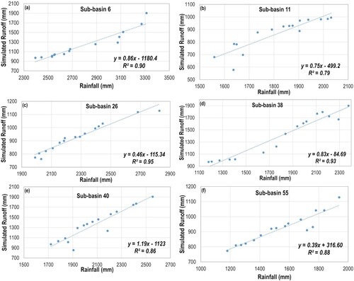
3.7. Estimation of correlation between rainfall and simulated runoff

The present study analyzes the relationship between rainfall and simulated runoff by estimating the correlation coefficient using linear regression for each sub-basin (Subramanya, 2006; Tirkey et al., 2014). The value of R² for each sub-basin is greater than 0.80, which shows that a strong correlation exists between rainfall and runoff depth (Supplementary Table S2). The result of the linear regression is illustrated for some of the sub-basins (Figure 6a-f).

Figure 6. Correlation between rainfall and simulated runoff depth.

This figure consists of 6 figures showing a graphical representation of the correlation between rainfall and runoff depth for the sub-basins 6, 11, 26, 38, 40, and 55. The coefficient of determination value for all the selected sub-basins is greater than 0.80 which suggests that the parameters are strongly correlated.

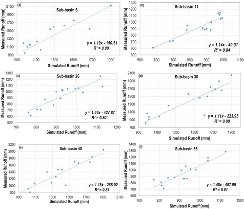
3.8. Estimation of correlation between simulated and measured runoff depth

The correlation between the measured and simulated runoff is estimated for each sub-basin, and the value of R² is found to be greater than 0.80. It shows that the measured runoff of each sub-basin is strongly correlated with the simulated runoff (Supplementary Table S2). The correlation coefficient values of sub-basin 6,11, 26, 38, 40, and 50 are shown ((Figure 7a-f)).

Figure 7. Correlation between simulated and measured runoff depth.

This figure consists of 6 figures showing a graphical representation of the correlation between simulated and measured runoff depth for the sub-basins 6, 11, 26, 38, 40, and 55. The coefficient of determination value for all the selected sub-basins is greater than 0.80 which suggests that the parameters are strongly correlated.

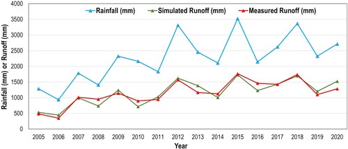
The temporal variation among rainfall, simulated, and measured runoff from 2005 to 2020 shows that with the increase in precipitation, the simulated and measured runoff depth is also increasing (Figure 8).

Figure 8. Temporal variation of rainfall, simulated and measured runoff depth.

This figure represents the temporal variation of rainfall, simulated and measured runoff depth for the present study. Long Description: In this figure represents temporal variation and relation between rainfall, simulated and measured runoff depth from 2005 to 2020. It shows linear relation exists in rainfall, simulated and measured runoff depth.

3.9. Validation of the model

The NSE assessment reveals that the NRCS-CN method is efficient and reliable in predicting runoff depth for the Assam region. The range of the NSE coefficient estimated for the study area lies between 0.623–0.786 (Supplementary Table S2). According to Moriasi et al. (2007), the model's performance falls under the satisfactory class for NSE coefficient values ranging between 0.50–0.70, and in the good class from 0.70–0.80. Out of 63 sub-basins, the NSE value of 45 sub-basins falls under the good category.

4. Discussion

For effective flood risk management in flood-prone regions like Assam, it is essential to analyze the relationship between precipitation and runoff within a watershed. LULC and soil condition of land affect its infiltration capacity, and surface runoff occurs when precipitation rates exceed the infiltration rate. (Bal et al., 2021; Bera et al., 2021; Deshmukh et al., 2013; Satya et al., 2020). The study results indicate that the NRCS-CN model is effective and reliable for the Assam region, and it can also be applied to other areas with a high potential of waterlogging during heavy rainfall scenarios. The areas with the dominance of soil groups like HSG C and HSG D, with low infiltration rates, and settlement areas with impervious land experience higher runoff (Akbari et al., 2021; Kumari et al., 2019). For some parts of the study area, the effect of surface slope variation is also shown on the curve number estimation (Ajmal et al., 2016; Ebrahimian et al., 2012; Garg et al., 2013). The correlation coefficient estimated for the rainfall vs. simulated runoff and simulated runoff vs. measured runoff of each sub-basin shows a strong positive correlation and the results are comparable with the studies conducted by Al-Ghobari et al. (2020), Zhang (2019), Ajmal et al. (2016), Chanu et al. (2015), and Tirkey et al. (2014). The strong positive correlation obtained in the present study enhances the suitability of the NRCS-CN model to estimate surface runoff. Further, the model's efficiency is examined by carrying out an NSE assessment for each sub-basin, and the majority of the correlation value falls under the good category (Oliveira et al., 2016;). It is also evident that geospatial techniques can aid in establishing the precise relationship between rainfall and runoff by providing accurate information on watershed characteristics located in rugged and inaccessible terrains (Verma et al., 2017; Zhang, 2019). The study also shows that social and ecological components of a system interact in a complex and non-linear manner. It is essential to give attention to better irrigation practices, water conservation policies, developments of green urban spaces, and improvement of drainage networks.

5. Conclusion

The present study conducts runoff estimation for the Assam region using the GIS-based NRCS-CN method. The study area is divided into 63 sub-basins, and the LULC-HSG complex is generated using GIS for each sub-basin. The study area shows the dominance of forest and agricultural land with HSG C and HSG B types of soils. The mean annual rainfall is estimated from 2005 to 2020, and the study area receives a relatively good amount of precipitation ranging from 936 mm to 3520 mm. For each LULC-HSG complex, CNI, CNII, and CNIII for AMC-I, AMC-II, and AMC-III, respectively, are estimated and are further corrected according to the surface slope variation. It is found that higher values of CN are associated with steeper slopes. The rainfall and simulated runoff of each sub-basin are strongly correlated with R² greater than 0.800. A similar result is observed for the correlation coefficient between simulated and measured runoff depth for each sub-basin. The runoff depth for the study area ranges from 1960 to 444 mm. Moderate to very high runoff is observed in the Lower Assam, very low to high range in the Northern and Upper Assam, and very low to low for Central Assam. The study also reveals that the spatial variation of runoff depends on the distribution of LULC, soil permeability, and rainfall intensity. The value of the NSE coefficient of each sub-basin also suggests that the model's performance falls from satisfactory to good. Compared with the conventional hydrological method, the NRCS-CN method is more suitable for estimating rainfall-induced surface runoff for the Assam region.

Estimation of surface runoff is critical as it demands accurate LULC, soil, meteorological conditions, and assigning correct CN values. The use of remote sensing and GIS helps in the extraction and simulation of the required parameters and provides a better technique to estimate the hydrological characteristics of the watershed. The result of the study helps to understand the rainfall-runoff behavior of the study area. It will also enhance the development of water resources and flood management systems at the sub-basin or watershed level by integrating remote sensing and GIS applications where data availability is limited.

Software

ESRI ArcGIS 10.5 is used for the spatial analysis of data, generation of different layers used in the study, and calculation of the estimated parameters.

DEM data of the study area is derived from; https://earthexplorer.usgs.gov/

Soil data is obtained from; https://www.fao.org/soils-portal/data-hub/soil-maps-and-databases/harmonized-world-soil-database-v12/en/ in the vector format.

Daily Gridded Rainfall Data with a Spatial Resolution of 0.25×0.25 is collected from; https://www.imdpune.gov.in/Clim_Pred_LRF_New/Grided_Data_Download.html.

LULC map is extracted from; https://livingatlas.arcgis.com/landcover/

Google Earth Pro is utilized for the accuracy assessment of the LULC map.

The coordinate system utilized for the analysis is UTM-WGS 1984, zone 46N.

Declaration of Competing Interests

The authors declare that they have no known competing financial interests or non-financial interests or personal relationships that are directly or indirectly related to the work submitted for publication that could have appeared to influence the work reported in this paper.

Data Availability Statement

The authors confirm that the data supporting the findings of this study are available within the article and some of the raw data were generated at our laboratory and derived data supporting the findings of this study are available upon reasonable request.

Disclosure statement

No potential conflict of interest was reported by the author(s).

References

- Abdessamed, D., & Abderrazak, B. (2019). Coupling HEC-RAS and HEC-HMS in rainfall–runoff modeling and evaluating floodplain inundation maps in arid environments: Case study of Ain sefra city. Ksour Mountain. SW of Algeria. Environmental Earth Sciences, 78(19), 1–17. https://doi.org/10.1007/s12665-019-8604-6
- Agrawal, N., Gupta, L., & Dixit, J. (2021). Assessment of the socioeconomic vulnerability to seismic hazards in the national capital region of India using factor analysis. Sustainability, 13(17), 9652. https://doi.org/10.3390/su13179652
- Ajmal, M., Waseem, M., Ahn, J. H., & Kim, T. W. (2016). Runoff estimation using the NRCS slope-adjusted curve number in mountainous watersheds. Journal of Irrigation and Drainage Engineering, 142(4), 04016002. https://doi.org/10.1061/(ASCE)IR.1943-4774.0000998
- Akbari, A., Daryabor, F., Abu Samah, A., & Shirmohammadi Aliakbarkhani, Z. (2021). Improving runoff estimation by raster-based natural resources conservation service-curve number adjustment for a new initial abstraction ratio in semi-arid climates. River Research and Applications, 37(9), 1333–1342. https://doi.org/10.1002/rra.3840
- Al-Ghobari, H., Dewidar, A., & Alataway, A. (2020). Estimation of surface water runoff for a semi-arid area using RS and GIS-based SCS-CN method. Water, 12(7), 1924. https://doi.org/10.3390/w12071924
- Bal, M., Dandpat, A. K., & Naik, B. (2021). Hydrological modeling with respect to impact of land-use and land-cover change on the runoff dynamics in budhabalanga river basing using ArcGIS and SWAT model. Remote Sensing Applications: Society and Environment, 23, 100527. https://doi.org/10.1016/j.rsase.2021.100527
- Bera, D., Kumar, P., Siddiqui, A., & Majumdar, A. (2021). Assessing impact of urbanisation on surface runoff using vegetation-impervious surface-soil (VIS) fraction and NRCS curve number (CN) model. Modeling Earth Systems and Environment, 1–14. https://doi.org/10.1007/s40808-020-01079-z
- Caloiero, T., Coscarelli, R., & Pellicone, G. (2020). A gridded database for the spatiotemporal analysis of rainfall in southern Italy (calabria region). Environmental Sciences Proceedings, 2(1), 6. https://doi.org/10.3390/environsciproc2020002006
- Census of India. (2011). Census of India 2011 provisional population totals. Office of the Registrar General and Census Commissioner.
- Chanu, S. N., Thomas, A., & Kumar, P. (2015). Estimation of curve number and runoff of a micro-watershed using soil conservation service curve number method. Journal of Soil & Water Conservation, 14(4), 317–325.
- Deshmukh, D. S., Chaube, U. C., Hailu, A. E., Gudeta, D. A., & Kassa, M. T. (2013). Estimation and comparision of curve numbers based on dynamic land use land cover change, observed rainfall-runoff data and land slope. Journal of Hydrology, 492, 89–101. https://doi.org/10.1016/j.jhydrol.2013.04.001
- Devi, N. N., Sridharan, B., & Kuiry, S. N. (2019). Impact of urban sprawl on future flooding in chennai city, India. Journal of Hydrology, 574, 486–496. https://doi.org/10.1016/j.jhydrol.2019.04.041
- Dixit, J., Raghukanth, S. T. G., & Dash, S. K. (2016). Spatial distribution of seismic site coefficients for Guwahati city. In N. Raju (Ed.), Geostatistical and geospatial approaches for the characterization of natural resources in the environment (pp. 533–537). Springer. https://doi.org/10.1007/978-3-319-18663-4_80
- Ebrahimian, M., Nuruddin, A. A. B., Soom, M. A. B. M., Sood, A. M., & Neng, L. J. (2012). Runoff estimation in steep slope watershed with standard and slope-adjusted curve number methods. Polish Journal of Environmental Studies, 21(5), 1191–1202.
- Ebrahimian, M., See, L. F., Ismail, M. H., & Malek, I. A. (2009). Application of natural resources conservation service–curve number method for runoff estimation with GIS in the kardeh watershed, Iran. European Journal of Scientific Research, 34(4), 575–590.
- Farran, M. M., Elfeki, A., Elhag, M., & Chaabani, A. (2021). A comparative study of the estimation methods for NRCS curve number of natural arid basins and the impact on flash flood predications. Arabian Journal of Geosciences, 14(2), 1–23. https://doi.org/10.1007/s12517-020-06341-3
- Farran, M. M., & Elfeki, A. M. (2020). Statistical analysis of NRCS curve number (NRCS-CN) in arid basins based on historical data. Arabian Journal of Geosciences, 13(1), 1–15. https://doi.org/10.1007/s12517-019-4993-9
- Garaga, R., Chakraborty, S., Zhang, H., Gokhale, S., Xue, Q., & Kota, S. H. (2020). Influence of anthropogenic emissions on wet deposition of pollutants and rainwater acidity in guwahati, a UNESCO heritage city in northeast India. Atmospheric Research, 232, 104683. https://doi.org/10.1016/j.atmosres.2019.104683
- Garg, V., Nikam, B. R., Thakur, P. K., & Aggarwal, S. P. (2013). Assessment of the effect of slope on runoff potential of a watershed using NRCS-CN method. International Journal of Hydrology Science and Technology, 3(2), 141–159. https://doi.org/10.1504/IJHST.2013.057626
- Gupta, L., Agrawal, N., & Dixit, J. (2021). Spatial distribution of bedrock level peak ground acceleration in the national capital region of India using geographic information system. Geomatics, Natural Hazards and Risk, 12(1), 3287–3316. https://doi.org/10.1080/19475705.2021.2008022
- Gupta, L., & Dixit, J. (2022). A GIS-based flood risk mapping of Assam, India, using the MCDA-AHP approach at the regional and administrative level. Geocarto International, 1–33. https://doi.org/10.1080/10106049.2022.2060329.
- Hishe, S., Bewket, W., Nyssen, J., & Lyimo, J. (2020). Analysing past land use land cover change and CA-markov-based future modelling in the middle suluh valley, Northern Ethiopia. Geocarto International, 35(3), 225–255. https://doi.org/10.1080/10106049.2018.1516241
- Huang, M., Gallichand, J., Wang, Z., & Goulet, M. (2006). A modification to the soil conservation service curve number method for steep slopes in the loess plateau of China. Hydrological Processes, 20(3), 579–589. https://doi.org/10.1002/hyp.5925
- Karra, K., Kontgis, C., Statman-Weil, Z., Mazzariello, J. C., Mathis, M., & Brumby, S. P. (July 2021). Global land use/land cover with sentinel 2 and deep learning. In 2021 IEEE international geoscience and remote sensing symposium IGARSS (pp. 4704–4707). IEEE.
- Karunanidhi, D., Anand, B., Subramani, T., & Srinivasamoorthy, K. (2020). Rainfall-surface runoff estimation for the lower bhavani basin in south India using SCS-CN model and geospatial techniques. Environmental Earth Sciences, 79(13), 1–19. https://doi.org/10.1007/s12665-020-09079-z
- Koneti, S., Sunkara, S. L., & Roy, P. S. (2018). Hydrological modeling with respect to impact of land-use and land-cover change on the runoff dynamics in Godavari river basin using the HEC-HMS model. ISPRS International Journal of Geo-Information, 7(6), 206. https://doi.org/10.3390/ijgi7060206
- Kumar, P. S., Praveen, T. V., & Prasad, M. A. (2016). Rainfall–runoff modelling using modified NRCS-CN. RS and GIS–A Case Study. Journal of Engineering Research and Applications, 6, 54–58.
- Kumar, R. (2021). Advances in remote sensing for natural resource monitoring, India. Advances in Remote Sensing for Natural Resource Monitoring, 389–404. https://doi.org/10.1002/9781119616016.ch19
- Kumari, R., Mayoor, M., Mahapatra, S., Parhi, P. K., & Singh, H. P. (2019). Estimation of rainfall-runoff relationship and correlation of runoff with infiltration capacity and temperature over east singhbhum district of jharkhand. International Journal of Engineering and Advanced Technology, 9(2), 461. https://doi.org/10.35940/ijrte.B3216.129219
- Lian, H., Yen, H., Huang, J. C., Feng, Q., Qin, L., Bashir, M. A., Wu, S., Zhu, A. X., Luo, J., Di, H., & Lei, Q. (2020). CN-China: Revised runoff curve number by using rainfall-runoff events data in China. Water Research, 177, 115767. https://doi.org/10.1016/j.watres.2020.115767
- Mishra, S. K., Singh, V. P., & Singh, P. K. (2018). Revisiting the soil conservation service curve number method. In V. Singh, S. Yadav, & R. Yadav (Eds.), Hydrologic modeling. Water Science and Technology Library (Vol. 81, pp. 667–693). Springer. https://doi.org/10.1007/978-981-10-5801-1_46
- Mohammad, F. S., & Adamowski, J. (2015). Interfacing the geographic information system, remote sensing, and the soil conservation service–curve number method to estimate curve number and runoff volume in the asir region of Saudi Arabia. Arabian Journal of Geosciences, 8(12), 11093–11105. https://doi.org/10.1007/s12517-015-1994-1
- Moriasi, D. N., Arnold, J. G., Van Liew, M. W., Bingner, R. L., Harmel, R. D., & Veith, T. L. (2007). Model evaluation guidelines for systematic quantification of accuracy in watershed simulations. Transactions of the ASABE, 50(3), 885–900. https://doi.org/10.13031/2013.23153
- Mukherjee, S., Bebermeier, W., & Schütt, B. (2018). An overview of the impacts of land use land cover changes (1980–2014) on urban water security of Kolkata. Land, 7(3), 91. https://doi.org/10.3390/land7030091
- Nash, J. E., & Sutcliffe, J. V. (1970). River flow forecasting through conceptual models part I — A discussion of principles. Journal of Hydrology, 10(3), 282–290. https://doi.org/10.1016/0022-1694(70)90255-6
- NRCS, U. (2004). National engineering handbook: Part 630—hydrology. USDA Soil Conservation Service.
- NRCS, U. (2009). Chapter 7–hydrologic soil groups. In NRCS–National Engineering Handbook (NEH), Part 630–Hydrology (pp. 7–1). USDA NRCS.
- Oliveira, P. T. S., Nearing, M. A., Hawkins, R. H., Stone, J. J., Rodrigues, D. B. B., Panachuki, E., & Wendland, E. (2016). Curve number estimation from Brazilian cerrado rainfall and runoff data. Journal of Soil and Water Conservation, 71(5), 420–429. https://doi.org/10.2489/jswc.71.5.420
- Pal, I., & Singh, S. (2018). Disaster risk governance and response management for flood: A case study of Assam, India. In I. Pal & R. Shaw (Eds.), Disaster risk governance in India and cross cutting issues. Disaster risk reduction (pp. 143–163). Springer. https://doi.org/10.1007/978-981-10-3310-0_8
- Pathak, S., Liu, M., Jato-Espino, D., & Zevenbergen, C. (2020). Social, economic and environmental assessment of urban sub-catchment flood risks using a multi-criteria approach: A case study in Mumbai city, India. Journal of Hydrology, 591, 125216. https://doi.org/10.1016/j.jhydrol.2020.125216
- Pathan, H., & Joshi, G. S. (2019). Estimation of runoff using SCS-CN method and ArcGIS for karjan reservoir basin. Int. J. Appl. Eng. Res. 14(12), 2945–2951.
- Patil, J. P., Sarangi, A., Singh, A. K., & Ahmad, T. (2008). Evaluation of modified CN methods for watershed runoff estimation using a GIS-based interface. Biosystems Engineering, 100(1), 137–146. https://doi.org/10.1016/j.biosystemseng.2008.02.001
- Psomiadis, E., Soulis, K. X., & Efthimiou, N. (2020). Using SCS-CN and earth observation for the comparative assessment of the hydrological effect of gradual and abrupt spatiotemporal land cover changes. Water, 12(5), 1386. https://doi.org/10.3390/w12051386
- Raghukanth, S. T. G., Dixit, J., & Dash, S. K. (2011). Ground motion for scenario earthquakes at guwahati city. Acta Geodaetica et Geophysica Hungarica, 46(3), 326–346. https://doi.org/10.1556/AGeod.46.2011.3.5
- Rajbanshi, J. (2016). Estimation of runoff depth and volume using NRCS-CN method in konar catchment (jharkhand, India). Journal of Civil and Environmental Engineering, 6, 10.4172. https://doi.org/10.4172/2165-784X.1000236
- Rao, K. N. (2020). A preliminary study of heavy metals pollution risk in water. Applied Water Science, 10(1), 1–16. https://doi.org/10.1007/s13201-019-1058-x
- Rawat, K. S., & Singh, S. K. (2017). Estimation of surface runoff from semi-arid ungauged agricultural watershed using SCS-CN method and earth observation data sets. Water Conservation Science and Engineering, 1(4), 233–247. https://doi.org/10.1007/s41101-017-0016-4
- Rawat, K. S., Singh, S. K., Singh, M. I., & Garg, B. L. (2019). Comparative evaluation of vertical accuracy of elevated points with ground control points from ASTERDEM and SRTMDEM with respect to CARTOSAT-1DEM. Remote Sensing Applications: Society and Environment, 13, 289–297. https://doi.org/10.1016/j.rsase.2018.11.005
- Ritter, A., & Munoz-Carpena, R. (2013). Performance evaluation of hydrological models: Statistical significance for reducing subjectivity in goodness-of-fit assessments. Journal of Hydrology, 480, 33–45. https://doi.org/10.1016/j.jhydrol.2012.12.004
- Rwanga, S. S., & Ndambuki, J. M. (2017). Accuracy assessment of land use/land cover classification using remote sensing and GIS. International Journal of Geosciences, 08(04), 611. https://doi.org/10.4236/ijg.2017.84033
- Sanz-Ramos, M., Martí-Cardona, B., Bladé, E., Seco, I., Amengual, A., Roux, H., & Romero, R. (2020). NRCS-CN estimation from onsite and remote sensing data for management of a reservoir in the eastern pyrenees. Journal of Hydrologic Engineering, 25(9), 05020022. https://doi.org/10.1061/(ASCE)HE.1943-5584.0001979
- Saran, S., Sterk, G., Aggarwal, S. P., & Dadhwal, V. K. (2021). Coupling remote sensing and GIS with KINEROS2 model for spatially distributed runoff modeling in a Himalayan watershed. Journal of the Indian Society of Remote Sensing, 49(5), 1121–1139. https://doi.org/10.1007/s12524-020-01295-1
- Satheeshkumar, S., Venkateswaran, S., & Kannan, R. (2017). Rainfall–runoff estimation using SCS–CN and GIS approach in the pappiredipatti watershed of the vaniyar sub basin, south India. Modeling Earth Systems and Environment, 3(1), 1–8. https://doi.org/10.1007/s40808-017-0301-4
- Satya, B. A., Shashi, M., & Pratap, D. (2020). Effect of temporal-based land use–land cover change pattern on rainfall runoff. In J. Ghosh & I. da Silva (Eds.), Applications of geomatics in civil engineering. Lecture notes in civil engineering (Vol. 33, pp. 175–182). Springer. https://doi.org/10.1007/978-981-13-7067-0_13
- Sharma, A., Rajbongshi, G., Alam, S. T., Rabha, D., Chamuah, K., Henbi, L. N., & Borah, B. (2020). Molecular typing of dengue viruses circulating in Assam, India during 2016–2017. Journal of Vector Borne Diseases, 57(3), 249. https://doi.org/10.4103/0972-9062.311779
- Shi, W., & Wang, N. (2020). An improved SCS-CN method incorporating slope, soil moisture, and storm duration factors for runoff prediction. Water, 12(5), 1335. https://doi.org/10.3390/w12051335
- Subramanya, S. (2006). Engineering hydrology. Tata McGraw-Hill Publishing Company Limited. 147–148.
- Taesiri, V., Pourkermani, M., Sorbi, A., Almasian, M., & Arian, M. (2020). Morphotectonics of Alborz province (Iran): A case study using GIS method. Geotectonics, 54(5), 691–704. https://doi.org/10.1134/S001685212005009X
- Talukdar, S., Singha, P., Mahato, S., Pal, S., Liou, Y. A., & Rahman, A. (2020). Land-use land-cover classification by machine learning classifiers for satellite observations—A review. Remote Sensing, 12(7), 1135. https://doi.org/10.3390/rs12071135
- Tian, J., Liu, J., Wang, Y., Wang, W., Li, C., & Hu, C. (2020). A coupled atmospheric–hydrologic modeling system with variable grid sizes for rainfall–runoff simulation in semi-humid and semi-arid watersheds: How does the coupling scale affects the results? Hydrology and Earth System Sciences, 24(8), 3933–3949. https://doi.org/10.5194/hess-24-3933-2020
- Tirkey, A. S., Pandey, A. C., & Nathawat, M. S. (2014). Use of high-resolution satellite data, GIS and NRCS-CN technique for the estimation of rainfall-induced runoff in small catchment of Jharkhand India. Geocarto International, 29(7), 778–791. https://doi.org/10.1080/10106049.2013.841773
- USDA, S. (1985). Hydrology, national engineering handbook, section 4. US Department of Agriculture.
- Verma, S., Verma, R. K., Mishra, S. K., Singh, A., & Jayaraj, G. K. (2017). A revisit of NRCS-CN inspired models coupled with RS and GIS for runoff estimation. Hydrological Sciences Journal, 62(12), 1891–1930. https://doi.org/10.1080/02626667.2017.1334166
- Vignesh, K. S., Anandakumar, I., Ranjan, R., & Borah, D. (2021). Flood vulnerability assessment using an integrated approach of multi-criteria decision-making model and geospatial techniques. Modeling Earth Systems and Environment, 7(2), 767–781. https://doi.org/10.1007/s40808-020-00997-2
- Zhang, W. Y. (2019). Application of NRCS-CN method for estimation of watershed runoff and disaster risk. Geomatics, Natural Hazards and Risk, 10(1), 2220–2238. https://doi.org/10.1080/19475705.2019.1686431
- Zhou, Y., Zhang, R., Wang, S., & Wang, F. (2018). Feature selection method based on high-resolution remote sensing images and the effect of sensitive features on classification accuracy. Sensors, 18(7), 2013. doi:10.3390/s18072013