A drift isopach model for the southwestern Great Slave Lake region, Northwest Territories, Canada

ABSTRACT

This study produced a drift thickness model for the southwestern Great Slave Lake area of northern Canada, using 12,692 lithostratigraphic records (seismic shothole drillers’ logs, diamond drill holes, petroleum wells), and field observations. Numerous algorithms and modelling parameters were tested using 6122 records of absolute drift thickness, and based on a cross-validation analysis, an empirical Bayesian kriging K-Bessel detrended algorithm was found to produce the best fit. The final model, incorporating selected maximum and minimum thickness estimate data, produced a root mean square error of 4.98 m, with 94.8% of the data points within ±2 m of the modelled drift thicknesses. The model identifies widespread areas of drift >10 m thick, and prominent southeast-northwest aligned bedrock ramps. Karst structures buried by ≤73 m of drift were identified southwest of Great Slave Lake and appear to be aligned with regional fault systems like ore-associated karst at Pine Point. These may be the source of anomalous glacial sediment-derived base metal indicators collected proximally to the west. The most striking drift anomaly is in Cameron Hills where the eastern and northern margins are comprised of shale and siltstone bedrock overlain by 20–40 m of glacial sediments, but the central and western uplands have petroleum well logs identifying glacial sediments up to 400 m thick. In addition to mineral exploration, results of this study provide baseline data that can be used predictively by the petroleum industry in designing future seismic and drilling (casing depth) operations, and by those modelling groundwater sources and flow.

KEYWORDS:

• Drift thickness
• glacial sediments
• isopach map
• empirical Bayesian kriging
• lithostratigraphy
• Northwest Territories

Key policy highlights

• Use of various lithostratigraphic records (petroleum wells, diamond drill holes, seismic shothole drillers’ logs) along with field observations highlights the strength of utilizing such archival data for research on regional glacial histories and sedimentology, for application to seismic exploration and well development, and for environmental assessments.

• Differential thicknesses of drift materials record widespread areas of shallowly buried bedrock, and thick (≤400 m) glacial deposits that comprise much of the Cameron Hills upland and has relevance to understanding regional hydrology.

• Distribution of glacial sediments and the identification of karst structures has application to understanding regional mineral drift prospecting.

1. Introduction

Drift is a collective term used to describe unconsolidated sediments overlying bedrock. In most of Canada, like other glaciated regions, drift is comprised predominantly of glacial deposits (till, glacifluvial, glacilacustrine, glacimarine), overlain by largely minor postglacial fluvial, colluvial, and eolian sediments (Fulton, 1995). Understanding the nature, thickness, and distribution of drift cover in Canada has broad application to many different studies, examples of which include glacial history (Norris et al., 2018; Smith et al., 2006), mineral exploration (DiLabio & Coker, 1989; Knight & Kerr, 2007; Paulen et al., 2006), groundwater source assessment (Gao et al., 2006), and granular aggregate resources (Best et al., 2006; Smith et al., 2011).

Isopach maps of drift (or other geological units) are constructed using algorithms based on control points that produce interpolative regional 2D and 3D-reconstructions of units and regional geological thicknesses. They are mathematical models of reality that are heavily dependent on the spatial and density distributions of the control points used to construct them. Models are also dependent on data accuracy and geological complexity and require input from knowledge experts who may discern realistic geological trends (e.g. buried channel thalwegs) and assess incongruous data (Culshaw, 2005). Deciding which algorithm provides the best approximation of reality is based on various statistical measures that describe the relative ‘fit’ of the model to the input data. Isopach maps of drift thickness have a long history of use in geological studies (e.g. Shangguan et al., 2017; Thorleifson et al., 2019), and many different computer programs and algorithms have evolved to interpret data, including machine learning and artificial intelligence (e.g. Atkinson et al., 2020; Machado, 2019; Rowans et al., 2018; Smirnoff et al., 2008).

Using a variety of different lithostratigraphic records of drift thickness available from existing databases, and archives of paper/microfiche records and sediment samples, along with field observations, this study aims to create a drift thickness model for a large area of northwestern Canada. Construction of the model uses the tools and algorithms available with ArcGIS Pro (v. 2.9) Geostatistical Analyst.

1.1. Study area

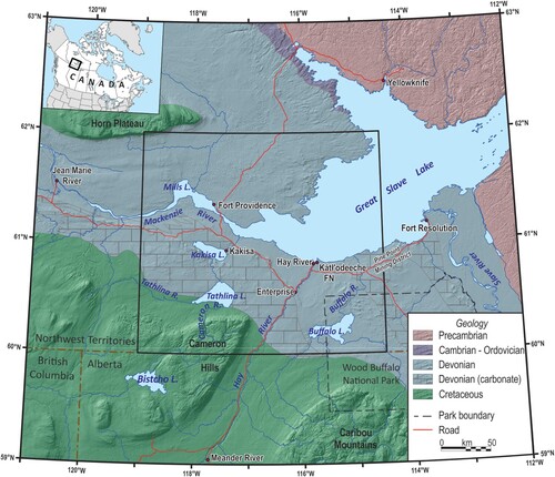
The ∼52,000 km² study area is situated in the southwestern Great Slave Lake region of southern Northwest Territories (NT), Canada (Figure 1). The area is comprised predominantly of flat to gently rolling, low-lying (150–300 m above sea level) taiga plains with extensive areas of sparsely tree-covered bog and fen, interspersed with white and black spruce and aspen poplar forests. Local rivers drain north into Great Slave Lake, which is the source of the west and then northward flowing Mackenzie River. The Cameron Hills, situated in the southwest part of the study area, rise over 550 m above the surrounding plains, and are a Cretaceous shale and siltstone bedrock-cored upland that extends southwards into Alberta and includes thick glacial drift (Dixon, 1999; Green et al., 1970; Pawlowicz et al., 2007). Beyond the Cameron Hills, flat lying to shallowly westward-dipping Devonian limestone reef complexes, platform carbonates, siltstone and shale characterize the regional geology (Figure 1; Okultich, 2006). Bedrock outcrops occur along a prominent southeast-northwest aligned, 15–25 m high carbonate escarpment ∼20 km south of Great Slave Lake, as isolated bedrock knobs south of Kakisa Lake and west of Buffalo Lake, along the channel walls of the lower Hay River, including 32 m high Alexandra Falls (10 km southwest of Enterprise), and at sporadic sites near the western shore of Great Slave Lake. The Laurentide Ice Sheet covered the area during the last (Late Wisconsinan) glaciation (∼25–10 ¹⁴C ka BP; Dyke, 2004; Lemmen et al., 1994), and southwest to west-flowing ice deposited extensive blankets of till across much of the region (Oviatt et al., 2015; Smith & Lesk-Winfield, 2010a).

Figure 1. Southern Northwest Territories study area and adjoining regions of Alberta and British Columbia. The central black box outlines the main study area, while full extents of Figure 1 are outlined in the Index Map (upper left). Simplified regional geology (adapted from Wheeler et al., 1996) overlies a hillshade model that highlights the full extent of the Cameron Hills uplands. Summit elevations of Horn Plateau, Cameron Hills, and Caribou Mountains are 881, 893, and 1030 m above sea level (asl), respectively. The surface of Great Slave Lake is 156 m asl.

An hillshade map showing the location, physiography, and bedrock geology of the study area, with towns and major lakes and rivers labelled.

2. Data

Several sources of data, that constrain the thickness and character of drift overlying bedrock, were used to create a drift isopach model. These included seismic shothole drillers’ logs (n = 18,009), mineral exploration diamond drill hole (DDH) records (n = 974), and petroleum well petrophysical logs, well cuttings, and well reports (n = 125). Water well records, which have been used in other regional drift and geological reconstructions (e.g. Hickin et al., 2008; Russell et al., 2006), were unavailable in this study area, reflecting its sparse population, abundant surface water, and the presence of discontinuous permafrost (e.g. VanGulck, 2016).

2.1. Data classes

It is important to recognize that the data types used to constrain drift thicknesses in this study include three different classes of information. The first are records that identify an exact depth for the contact between drift and underlying bedrock; these provide an absolute measure of drift thickness. In areas of particularly thick drift, and where boreholes are shallow, bedrock may not have been reached at the bottom of the hole. In these cases, records are considered minimum estimates of drift thickness (e.g. shothole log 0–20 m sand, clay, gravel; drift is >20 m thick). Where bedrock is encountered, but the log does not identify its actual depth (e.g. shothole log, 0–20 m clay, rocks, shale; interpreted to represent ‘till’ (clay, rocks) overlying shale (bedrock)), these records provide maximum estimates of drift thickness (i.e. shale bedrock occurs at a depth ≤20 m). Table 1 provides the abundance and types of each data source and class available within the bounds of the study area, and those used in creation of the drift isopach model. To reduce ‘edge effects’ in the spatial interpolative model and final map, an ∼8 km buffer zone of additional shothole drillers’ log records to the west and north was included (n = 3126; Table 1; this type of data does not extend to the south and east). The main study area is defined by geographic bounds 60°–62°N; 119°–114°30’W, and reflects the focus of fieldwork, surficial mapping, and data extents.

Table 1. List and abundance of drift thickness record types used in this study.

DATA TYPE	Total # of Records	# Absolute Depths	# Minimum Estimates	# Maximum Estimates
Shotholes (all)	10,468 (18,009)	3649 (3906)	6488 (10,751)	331 (3352)
Shotholes (buffer zone)	1849 (3126)	322 (322)	1518 (2037)	9 (767)
Diamond Drill Holes	970 (974)	962 (962)	8 (9)	0 (3)
Petroleum Wells	125	125	0	0
Field/Map data	1129 (1130)	1129 (1129)	0	0 (1)

Notes: Records in bold represent totals used in the final isopach model. Values in brackets represent total number of records present in study (and buffer zone) area. ‘Shotholes (all)’ values include the shothole records from the buffer zone.

2.2. Seismic shothole drillers’ logs

During the course of geophysical seismic exploration, shotholes are drilled (∼8–20 m deep) to set explosive charges. Drillers log the materials being drilled through at varying degrees of resolution and accuracy, and this information is used to determine whether the charge is seated in bedrock, or unconsolidated drift, as this influences signal transmission and static interference (Smith, 2012). These lithostratigraphic records were largely unknown and unavailable in Northwest Territories until a comprehensive project amassed all industry-held archival seismic shothole drillers’ log records from Northwest Territories and Yukon into publicly accessible Access databases and GIS (∼360,000 records; Smith, 2011, 2015; Smith & Farineau, 2015).

While shothole drillers’ logs are the most abundant lithostratigraphic logs of any kind in Northwest Territories, caution is urged in their use and interpretation. Smith (2011) outlined many considerations for interpreting and using these data, chief amongst them in relation to the present study is that shothole depths are generally shallow (average 12.7 m in the present study area), and in some instances drillers have confused frozen sand or frozen clay as sandstone or shale, respectively. What the drillers were adept at, though, is noting bedrock where they definitively encountered it (e.g. till overlying limestone), and conditions that were ‘difficult’ which would include things like boulders (from which a glacial origin of drift can be discerned). An earlier version of a drift (and till) isopach map had been created for the continental Northwest Territories based largely on shothole drillers’ log records (Smith & Lesk-Winfield, 2010a). It should be noted, however, that this was based on an interim version of the shothole drillers’ log database (n = 275,871 records; Smith & Lesk-Winfield, 2010b). The present study utilized the final shothole database compilation (n = 343,989 records; Smith, 2011), which included many new records within the study area. Because of computational limitations, this earlier drift isopach model also truncated petroleum well records to no more than 20 m depth, for which thicker deposits were regarded simply as >18 m thick. As with any such record, drillers’ logs benefit from proximal correlation with other lithostratigraphic records.

2.3. Diamond drill holes

The study area contains the historic Mississippi Valley-type lead-zinc Pine Point mining district located south of Great Slave Lake and east of Buffalo River (Figure 1), which was operated by Cominco from 1964 to 1988. Ore deposits were extracted from 50 shallow open pits, formed within dolomitized limestone and karst structures (Hannigan, 2006). Drift thicknesses in the area range from near zero in the east along the Paleozoic-Precambrian (Canadian Shield) margin (Figure 1), to blankets of till up to 25 m thick (Oviatt et al., 2015; Rice et al., 2019). Inspection by the authors of recent drill cores from the Pine Point area by Pine Point Mining Ltd. reveals that drift infilling individual karst collapse structures can exceed 100 m total thickness (base of karst collapse to land surface). Exploration predating the Cominco mines and extensive regional exploration around the southwestern shores of Great Slave Lake during and following mining operation, searching for additional ore resources, resulted in many more diamond drill holes. Based on how they were drilled and logged, these diamond drill hole records provide what are considered the most accurate measures of drift thickness, and in some cases include characterizations of drift composition. Turner et al. (2002) compiled a database of 893 diamond drill hole logs from the Pine Point mining district based on exploration Assessment Reports that are archived online by the Northwest Territories Geological Survey (https://app.nwtgeoscience.ca/). The present study expands their geographical review of Assessment Reports to areas west of Hay River and Great Slave Lake (81 additional diamond drill hole records).

2.4. Petroleum well logs

The study area lies within the Western Canada Sedimentary Basin and has been the site of historical petroleum exploration and development (Mossop & Shetsen, 1994). In addition to associated seismic exploration (i.e. shothole drillers’ logs), there are several different sources of drift thickness records associated with petroleum wells (e.g. Janicki, 2005; Pawlowicz et al., 2007), including petrophysical logs (e.g. gamma, neutron, sonic, and resistivity), well site geology reports, and well cuttings. Where available, the petrophysical logs provide an accurate means of identifying the sharp geophysical/lithological contact between drift and underlying bedrock, and accurate depth measurements (Hickin et al., 2008). However, wells in the study area are almost always cased to depths below the drift-bedrock contact, so typically only the gamma-neutron logs could provide interpretable records through the casing, but even with these, recordings were typically only initiated at/below the casing depth. Interpretation of bedrock formation top contacts from petrophysical logs, including the drift-bedrock contact (e.g. Janicki, 2005), are best when correlated across records from several proximal wells. Wells in the study area, however, are typically isolated, and in most cases, there were no petrophysical records available, or the contacts were equivocal.

Well cuttings are pieces of bedrock and sediments recovered during the drilling process. These materials are carried to the surface within the drilling muds, passed across a shale shaker table/sluice box to remove fines (silt and clay), and then washed to remove the drilling muds. Samples of cuttings were originally collected by companies at 10 foot intervals, but this has now changed to 5 m intervals. Lithological and sedimentological descriptions of cuttings can sometimes be found in accompanying well site geology reports, from which the drift-bedrock contact can be ascertained (if collection of cuttings started at or near the surface, as opposed to those which start below the casing depth, i.e. below the drift-bedrock contact). A digital and paper archive of onsite publicly available well reports at the Geological Survey of Canada (GSC), Calgary office, was reviewed for all Northwest Territories wells in the study area. Microfiche copies of these well reports are also publicly available onsite at the Canada Energy Regulator, Calgary office. A large collection of cuttings for Northwest Territories wells is also archived and accessible at the GSC Calgary office, and these were similarly inspected. Identification of the drift-bedrock contact based on cuttings can range from sharp to equivocal, as contamination can occur from caving of unconsolidated and other material in the well bore, and in cases, overlying drift can extend downwards tens of metres through bedrock cuttings. Where the upper limits of bedrock are deeply weathered it can be difficult to discern this contact from glacial reworking of local bedrock material. As a course of practice, the first instance where bedrock (e.g. shale) appeared in abundances >10% of the cuttings and where the bedrock composition steadily increased thereafter, was picked as the upper bedrock contact. We have modified many of the formation top picks of Janicki (2005) based on our detailed inspection of the well cuttings and well reports and have added new petroleum well records and those that had not been included by Janicki (2005) or were previously unavailable.

2.5. Field observations/surficial geology maps

Our study included control points (n = 1129; Table 1) for areas where fieldwork identified bedrock at surface (0 m drift thickness), where bedrock outcropped along stream channels and quarry exposures (variable depths), and areas of till or other sediment veneer overlying bedrock (≤2 m drift thickness; Hagedorn et al., 2022, in press; Paulen & Smith, 2022; Smith et al., 2017, 2021, in press). Note that areas of veneer (including large areas along the western shore of Great Slave Lake) were input as 2 m in the model, even though by definition, veneer includes areas with drift cover ranging from 0 to 2 m.

3. Methodology

This study used the deterministic and geostatistical methods available in the Geostatistical Analyst function in ArcGIS Pro (v 2.9; https://pro.arcgis.com/en/pro-app/latest/help/analysis/geostatistical-analyst/) to create surfaces (model outputs) of drift thickness. Different algorithms are suited to different types of data, spatial contexts, and desired outputs (e.g. spatial smoothing), and govern whether points are treated deterministically (i.e. whether the model forces the surface to coincide with the data point or not, such as Inverse Distance Weighting), or geostatistically such as kriging which provides statistical interpolation of the model surface and measured points. There are a wide range of data parameters considered in each model type, many of which relate to the kernel weighting function that assigns differential weights to values close to where a prediction is being made, versus those situated further away (e.g. subset size, number of neighbours, sector type, and radius size). We tested the different algorithms by using combinations and permutations of the different data parameters available for Natural Neighbour, Inverse Distance Weighting, Kriging, and Empirical Bayesian Kriging.

Models were constructed originally using only the dataset of 6122 points considered to represent absolute measures of drift thickness (note, 256 points from southern Cameron Hills were later removed; discussed below). We initially tested, but ultimately rejected using the Geostatistical Analyst ‘training set’ method, in consideration of the overall small number and spatial variability of data points, and the extreme variations in sediment thicknesses in short proximity to one and other particularly in areas for which there was very little data control (e.g. Cameron Hills where isolated and adjacent points have upwards of 400 m drift thickness differences; removal of one or more of these points produced significantly different drift models). Instead, we employed the ‘cross validation’ method in Geostatistical Analyst which provides iterative testing of a model’s accuracy. With cross validation, the model leaves a point out, and then uses all others to predict a value at that same location. This is iteratively carried out for all the input data points. Results of ‘predicted’ versus ‘known’ values are provided and summarized statistically by the measure of root mean square error (RMSE). The lower the root mean square error, the greater the accuracy of the output model relative to the input data.

In addition to root means square error, empirical Bayesian kriging provides a further cross validation summary statistic of ‘Inside 90 Percent Interval’ and ‘Inside 95 Percent Interval’. These statistics assess the consistency of standard errors with predicted values and should be close to 90/95. Where measures are greater than 90/95, then the standard errors are too large relative to predicted values, and when below 90/95, the standard errors are too small (ArcGIS Pro; https://pro.arcgis.com/en/pro-app/latest/help/analysis/geostatistical-analyst/).

4. Results

Models were contrasted based on their root mean square error (except the deterministic Natural Neighbour method for which root mean square error is not calculated). The empirical Bayesian kriging models were also ranked by their inside 90 and 95 percent interval values. All the models were also visually assessed based on our field observations and geological understanding of the region. Ten iterations of Natural Neighbour, 19 Inverse Distance Weighting, 34 Kriging, and 63 Empirical Bayesian Kriging were run. Examples of what are considered the best fit/lowest root mean square error models are displayed in Figure 2.

Figure 2. Examples of different algorithms tested for best-fit to the 6122 absolute drift thickness data points in the southwest Great Slave Lake study area. Individual models are plotted using the same topographic and hydrological bases and drift thickness colour gradations shown in 2A. Contour interval 100 m; Great Slave Lake elevation 156 m asl. 2A – Natural Neighbour. 2B – Inverse Distance Weighting; root mean square error (RMSE) = 6.65. 2C – Simple Exponential Kriging; RMSE = 7.37. 2D – Empirical Bayesian Kriging (K-Bessel detrended); RMSE = 6.55.

(A) A contour map of the study area showing the pattern of colour gradient shaded drift thicknesses produced using a Natural Neighbour algorithm. (B) A contour map of the study area showing the pattern of colour gradient shaded drift thicknesses produced using a Inverse Distance Weighting algorithm. (C) A contour map of the study area showing the pattern of colour gradient shaded drift thicknesses produced using a Simple Kriging algorithm. (D) A contour map of the study area showing the pattern of colour gradient shaded drift thicknesses produced using an Empirical Bayesian Kriging algorithm.

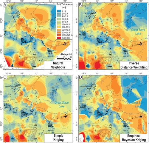
An empirical Bayesian kriging K-Bessel detrended algorithm was selected as providing the lowest root mean square error, and the most visually ‘true’ sense of our geological understanding of the study area. It used the following parameters: Transformation Type – Empirical; Semivariogram Model type – K-Bessel detrended; Subset size – 200; Overlap Factor – 1; Number of Simulations – 100, Searching neighbourhood – standard circular; Neighbours to include – 8; Include at least – 2; Sector type – 1; Radius – 50 m. Our best-fit empirical Bayesian kriging model had a root mean square error of 6.55 m, with inside 90 and 95 percent interval values of 89.25 and 92.96, respectively.

Having established a best-fit model using the absolute thickness data, interpolated model thickness measurements were then compared against all the maximum drift thickness estimate data points. Where the model predicted drift thicknesses greater than maximum estimates (331 of 3355 data records; Table 1), these data (using the total hole depths; which are acknowledged as overestimates) were input to pull the model thicknesses up (Figure 3(a)), and then the model was re-run. This slightly improved the root mean square error to 6.46 m (inside 90 and 95 percent interval values of 89.63 and 93.21). This revised model was then similarly tested against all the minimum estimate data points (n = 10,760; Table 1), for which predicted depths were less than the minimum estimates at 6496 sites. These were added to the dataset (also using the total hole depths; acknowledged as underestimates; Figure 3(a)), and the model was re-run using the same parameters, producing a root mean square error of 5.40 m (inside 90 and 95 percent interval values of 90.34 and 92.94). Finally, we removed 256 ‘absolute/maximum thickness estimate’ seismic shothole drillers’ log records (shothole depths = 13.1 m) from a cluster of 5 seismic lines in southwest Cameron Hills, bordering Alberta (Figure 3(a)). These records of seemingly shallow bedrock are sharply contradicted by drift thicknesses in 3 adjoining wells in Northwest Territories (400 and 391 m (8 km to the west) and 94.5 m (12 km to the northeast)) and >100 wells across the border in Alberta (Utting et al., in prep.) that demonstrate a broad area of thick drift (>200 m) overlying the central and western Cameron Hills and surrounding upland region. We suggest that shothole records of sandstone (n = 235) and shale (n = 21) made by drillers in these 5 seismic lines are a misattribution of the dominant sedimentology within the drift cover and may correspond to frozen sand and frozen clay (till). Stereo air photograph interpretation indicates that the area covered by these seismic lines includes extensive regions of thermokarst and ice-cored raised peat plateau, overlying streamlined till and glacifluvial outwash. Field investigations elsewhere on Cameron Hills identified stratified till with shale-rich diamict and coarse sand and gravel interbeds, while well cuttings in the adjacent 3 wells indicate abundant sand throughout their record. We acknowledge the selectivity of removing these records but argue that this does not call into question the accuracy of other shothole records. Were there a systematic, or even common error, we would expect to see it repeated throughout the survey. Instead, field observations broadly agree with the shothole log records, as do all but perhaps 3 other of the 125 petroleum well records (discussed below). With this change, and by increasing the number of simulations from 100 to 500 and subset size from 200 to 500, the final drift isopach model (see Main Map) achieved a root mean square error of 4.98 m, and inside 90 and 95 percent interval values of 90.58 and 93.04, respectively.

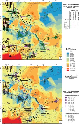
Figure 3. Distribution and classification of drift thickness records used in final model. (A) Distribution of the different data types and classes of the 20,238 total records, colour coded as to whether they were used or not. Records coloured green, fuchsia, and pink are absolute, minimum, and maximum records, respectively, that were used. Records depicted by black circles are minimum or maximum estimates that were not used. Site 1 corresponds to the records from 5 seismic lines on Cameron Hills removed from the final model compilation. (B) Assessment of whether the model underestimated the record thickness (purple circles) or overestimated the record thickness (green circles) for the 12 692 records used in the final model. Size of the circles is proportional to the relative estimate error. Total number of data records within each thickness over-, and under-estimate interval indicated in parenthesis. Numbered sites 1 to 11 are discussed in the text. Select exposed and shallowly buried bedrock units outlined by grey dashed lines include carbonate units: uDTF – Twin Falls Formation (includes Alexandra Falls Member), uDKA – Kakisa Formation, uDTR – Trout River Formation; and siltstone and shale unit: uDTA – Tathlina Formation; (adapted from Okultich, 2006).

(A) A colour-shaded drift thickness map of the study area in southern Northwest Territories that shows the distribution of all available data points. Individual points are distinguished by shape and colour to indicate the type of drift thickness record, and whether it was used in the final model, or not. (B) A colour-shaded drift thickness map of the study area in southern Northwest Territories that shows the distribution of data points used. The data points are represented by coloured circles that reflect whether the model over- (green) or underestimates (purple) the drift thickness. The size of the circles is proportional to how much the model over- or underestimates the measured thicknesses.

The drift isopach map is not contoured using a linear thickness scale. Rather, thickness intervals were chosen to reflect logical divisions of deposit thicknesses associated with regional field observations, surficial geology mapping, and natural breaks in the data distribution histogram, aspects of which can be considered artefacts of data sources (e.g. prescribed shothole depths).

5. Discussion

Examples of the four main algorithm types used (Figure 2) illustrate a broad correspondence between different models. Differences are most pronounced when comparing the weighting that individual points have (particularly anomalous thickness and isolated data points), and how the models extrapolate coverage into areas with no, or only sparse data control. While the lowest root mean square error models were selected for each algorithm type, differences in spatial sampling parameters used by the models accounts for some of these differences and can be seen in the relative degree that data points are isolated (bullseyes) or integrated into broader regional patterns.

Discrepancies between the final empirical Bayesian kriging drift isopach model predicted drift thicknesses and the actual records are summarized in Figure 3b. The root mean square error of 4.98 m gives a statistical measure of the fit of the semivariogram curve to the actual data distribution. Negative errors, i.e. where the model underestimates the ‘true’ data point values, are shown on Figure 3b in thickness proportionally sized purple circles, while those where the model overestimated drift thicknesses are shown in green. Errors are further summarized by indicating the number of records that fall within each thickness over/underestimate interval (Figure 3(b)). Of the 12,692 data points used in the model (excluding the 3126 points from the model’s input data buffer zone), 94.8% of the modelled thicknesses are within ±2.0 m of the actual data points, and 98% are within ±3.5 m.

As with any drift isopach model, artefacts exist as a consequence of spatially heterogeneous distributions of control points. Examples of this are seen in the northernmost central portion of the map where there is no data control (this includes much of the area of ribbed moraine northeast of Mills Lake; see Main Map; Brown et al., 2011), most of Great Slave Lake itself (other than a few well records in the southwest), and the area around Buffalo Lake and upper Buffalo River (i.e. the area indicated as having 10–50 m thick drift). While a previous drift isopach model (Smith & Lesk-Winfield, 2010a) used 10 km buffers around points, and left areas beyond these blank, we have let the present study’s model extrapolate to a geographic bound defined by the data perimeter extents.

There are 13 data points for which the isopach model underestimates depths by >10 m, of which 8 are petroleum wells, and 5 are diamond drill holes (Figure 3(b) and Table 2). This includes 2 of the 7 well records on Cameron Hills (Figure 3(b), sites 1 and 2, and Table 2), in an area that has field observations of shallowly buried bedrock within 5–10 km of areas with drift litholog records up to 400 m thick. Site 2 (Figure 3(b)) also adjoins what field investigations revealed to be a deeply incised valley (up to 200 m deep) through which the Cameron River drains off Cameron Hills, that is floored by bedrock along its northern reaches, and is infilled by glacial sediments along its lateral margins (Smith et al., 2021). The drift thickness underestimates of these two Cameron Hills wells likely reflect spatial averaging/smoothing of sharply divergent data by the model. Elsewhere, there may be several explanations to account for petroleum well record and model discrepancies. East of Kakisa Lake (Figure 3(b), site 3, and Table 2), the well reports drift thickness of 27.4 m in an area that field investigations suggest extensive till veneer (drift thickness ≤2 m) and exposed bedrock. Examining the geology (Figure 3(b)), the bedrock outcrop sites all occur within areas underlain by Twin Falls and Kakisa formations limestone (uDTF and uDKA; Figure 3(b)), while the anomalous well sits within what is likely the recessive siltstone and shale Tathlina Formation (uDTA – Figure 3(b); Okultich, 2006). It is also suggested that the reported well drift thickness may have included weathered bedrock overlying more competent shale and may not have been corrected for the drilling rig kelly bushing datum vs actual ground surface elevation (an offset of ∼4 m; no information in well report). Assessing the question of weathered bedrock overlying competent bedrock is difficult. In the absence of actual drill core or detailed petrophysical logs for this site (which may discern density differences between the two strata), it would be overly subjective to interpret this from well cuttings, as with the mixing of cuttings and other inherent uncertainties, glacially reworked local bedrock and a weathered cap of bedrock could appear similar. Isolated well records at sites 4, 5, and 6 (Figure 3(b) and Table 2), adjacent to the upper Mackenzie River, seem quite disproportionate to surrounding wells and other drift thickness records. The well cuttings for each of these appears to be mostly till, thus dismissing the notion of thick weathered bedrock being confused for drift. It is possible that these anomalous depths reflect the presence of karst structures, particularly site 6 (164.6 m). Sites 7 and 8 (Figure 3(b) and Table 2) are well locations proximal to a 3D seismic array. Disparities between these two wells and the shothole drillers’ logs may reflect the proximal use of minimum thickness estimate data (Figure 3(a)), which is acknowledged to be an underestimate. It also likely reflects sediment thickness variabilities between glacitectonic ‘ribs’ and intervening swales of the mega-scale ribbed moraine swarm that these wells are situated in the western margin of (see Main Map; Brown et al., 2011; Dunlop & Clark, 2006).

Table 2. Drift thickness records from wells and diamond drill holes (DDH) for which the drift isopach model underestimates the measured thickness by >10 m.

DATA TYPE	Site #	Measured Depth (m)	Modelled Depth (m)
Well	1	400	388.0
Well	2	216.5	206.4
Well	3	27.4	7.2
Well	4	77.4	61.4
Well	5	91.4	76.5
Well	6	164.6	47.2
Well	7	36.6	16.8
Well	8	36.6	22.4
DDH	9	40.5	19.3
DDH	10	80.8	70.4
DDH	10	80.8	52.0
DDH	10	45.7	35.4
DDH	10	45.1	32.5

Note: Refer to Figure 3(b) for locations.

In the case of diamond drill hole site 9 (40.5 m; Figure 3(b) and Table 2) the Assessment Report identifies this as an overburden-filled karst structure (Lane, 1980), which is confirmed by our field observations of irregular bedrock outcrop topography, with intervening hollows partially infilled by bedrock (limestone) regolith and glacial sediments. Note, this area was submerged by glacial Lake McConnell during deglaciation (Lemmen et al., 1994), and would have been subject to significant wave washing and ice scour as the lake drained, contributing to the erosion of debris off topographic highs into intervening hollows.

Site 10 (Figure 3(b)), west of Buffalo River, includes a large cluster of diamond drill hole records in which 4 have their drift thicknesses underestimated by >10 m (Table 2). This region is known to include numerous karst structures (Turner et al., 2002) that diamond drill hole records reveal are infilled and overlain by 50–60 m and up to 88.4 m of drift. The upper regional bedrock contact in this area appears to lie ∼20–30 m below the drift surface, suggesting that the actual karst collapse structures are approximately 20–60 m deep, comparable to that observed in numerous open pits in the Pine Point mining district to the east (cf. Oviatt et al., 2015). Underestimates of drift thicknesses by the model likely reflect sharply divergent depths between the regional bedrock-drift contact, and karst collapse structures. Given the abundance of diamond drill hole records in this area, improved modelling of this local area could be derived by decreasing the radius of sampling to <50 m, and the subset size to <200 records. Visual distinction of the actual karst structures would require use of different drift thickness intervals.

Two prominent limestone benches that outcrop or are shallowly buried are clearly displayed in the drift isopach map (Figure 3(b) – blue shaded areas southwest of Great Slave Lake; Okultich, 2006). The first is the Twin Falls Formation (uDTF) that forms a bedrock escarpment and carbonate platform extending from east of Hay River, northwest across the region, sub-parallel to the southern Great Slave Lake shore, and then curves north of Kakisa Lake before terminating south of Mills Lake. Extensive outcrops of a second limestone bench occur south of Kakisa Lake (Trout River (uDTR) and Kakisa (uDKA) formations), and the trend of these units is depicted as extending from the eastern end of Tathlina Lake northwestward towards the Mackenzie River.

Additional karst structures, buried beneath thick drift (≤73 m from land surface to base of karst) are identified by diamond drill hole records southwest of Great Slave Lake (Figure 3(b), site 11). Interestingly, these are aligned with large regional fault systems (Hannigan, 2006; see Main Map) and are situated proximally glacially up-flow of anomalous sphalerite (ZnS) and galena (PbS) indicator mineral concentrations recovered from surface till and stream sediment samples (Paulen et al., 2018).

The Cameron Hills documents the greatest anomaly in terms of regional drift thicknesses in the study area. While bedrock outcrops were documented in the field along the northern and eastern rims of the upland (buried by up to 40 m of glacial sediments), petroleum well petrophysical logs, well-site geology reports, and well cuttings demonstrate an extensive and very thick (upwards of 400 m) drift cover. This tremendous infill of drift extends throughout the central and western limits of the upland in Northwest Territories, and for most of the contiguous upland area extending into Alberta (Utting et al., in prep.). A lithological and textural assessment of well cuttings, and petroleum well drillers’ reports of encountering boulders down to the base of many drift records, indicates that this drift is likely to be mostly glacial in origin (till and possibly glacifluvial). Buried pre-glacial fluvial thalwegs and associated sediments, however, are suggested to underlie parts of the Cameron Hills upland in Alberta, and in areas of northeastern British Columbia (Atkinson et al., 2020; Hickin et al., 2008).

6. Conclusions

Using a spatially disparate database of 3 different types of lithostratigraphic records along with field observations, an empirical Bayesian kriging (K-Bessel detrended) algorithm produced the lowest root mean square error (4.98 m) drift isopach model for the study area. The model appears to provide a realistic depiction of drift thicknesses, identifying areas of karst and thick glacial sediment cover, areas of shallowly buried and outcropping limestone bedrock, and a much less extensive bedrock core underlying the northern and eastern regions of Cameron Hills in Northwest Territories. The broader Cameron Hills uplands are instead revealed to be comprised of thick (≤400 m) Quaternary glacial sediments (till and/or glacifluvial). Only a few larger regions within the study area are devoid of lithostratigraphic control, and drift thickness projections here are considered modelling artefacts, and unreliable. For almost all other areas, agreement between the model and actual data points is considered excellent, and 94.8% of sites fall within ±2 m of their logged depths.

The drift isopach model provides an important reference for understanding regional glacial ice flow and sediment depositional/erosional histories. Thick till deposits (20–50 m) infill the terrain north of the regional bedrock escarpment, extending northwards of the Mackenzie River, perpendicular to the generally south and westward-flowing Late Wisconsinan Laurentide Ice Sheet. Karst bedrock structures (20–60 m deep) formed in dolomitized limestone (and the source of important lead and zinc ore resources), have been infilled by till, and further buried by 20–30 m of regional till cover resulting in total burial depths up to 88 m. The geological coincidence of several karst features at the west end of Great Slave Lake (south of Big Island), regional fault systems, and proximal anomalous base metal indicator mineral concentrations (Paulen et al., 2018), suggest that these may be potential lead/zinc ore exploration targets.

Software

Seismic shothole drillers’ logs were queried and extracted from a Microsoft Access database. All other lithostratigraphic data was compiled using Microsoft Excel. Drift isopach models were constructed using ArcGIS Pro (v. 2.9). Layers were exported as.eps files to CorelDRAW (v. X8) for final map and figure drafting. Digital elevation hillshade models are based on ArcticDEM (Porter et al., 2018) and CDEM tiles that were resampled at a 100 m cell size and processed using Global Mapper (v. 22.1) with a hillshade sun angle of 25° altitude and 315° azimuth.

Acknowledgements

This research was undertaken as part of Natural Resources Canada’s Geo-Mapping for Energy and Minerals (GEM-2) Program, Mackenzie Project, Southern Mackenzie Surficial activity. It was conducted under Northwest Territories Scientific Research Licence #16226. Wildlife monitors A. Farcy, J. Nadli, and H. Sabourin (Deh Gáh Got’ie First Nation), D. Simba (Ka’a’gee Tu First Nation), I. Graham and P. Martel (Kátł’odeeche First Nation), T. Unka (Denínu Kųę First Nation), and J. Delorme (Fort Resolution Métis Nation) are thanked for their participation and insight. Field assistance was provided by GEM-2 funded students R. King (Memorial University), J. Plakholm (Carleton University), and J. Sapera (Brock University). R. Fontaine (GSC Calgary) facilitated access to well cuttings and well report archives. P-M. Godbout (GSC Ottawa) provided an internal GSC review. Journal editor J. Knight and reviewers, E. Arnaud, S. Bernard, E. Phillips, and S. Wolfe are thanked for their edits and comments. This publication represents NRCan contribution #20220262.

Disclosure statement

No potential conflict of interest was reported by the author(s).

Data availability

Sources of the data used in this model are identified in the paper and can be accessed from publicly available electronic databases and digital scans of archived Assessment Reports, or from onsite review of archival paper well records and well cuttings housed at the Geological Survey of Canada (Calgary office). A compilation of all records used can be requested from the authors and will be made freely available in a future GSC Open File report, as part of an ongoing up-dated drift isopach reconstruction for Northwest Territories.

Additional information

Funding

This research was supported by Natural Resources Canada’s ‘Geo-mapping for Energy and Minerals (GEM-II)’ program, administered by the Geological Survey of Canada.

References

- Atkinson, L. A., Pawley, S. M., Andriashek, L. D., Hartman, G. M. D., Utting, D. J., & Atkinson, N. (2020). Bedrock Topography of Alberta, Version 2. AER/AGS, Map 610, scale 1:1 000 000. https://ags.aer.ca/data-maps-models/maps/map-610
- Best, M. E., Levson, V. M., Ferbey, T., & McConnell, D. (2006). Airborne electromagnetic mapping for buried Quaternary sands and gravels in northeast British Columbia. Journal of Environmental and Engineering Geophysics, 11(1), 17–26. https://doi.org/10.2113/JEEG11.1.17
- Brown, V. H., Stokes, C. R., & Ó Cofaigh, C. (2011). The glacial geomorphology of the north-west sector of the Laurentide Ice Sheet. Journal of Maps, 7(1), 409–428. https://doi.org/10.4113/jom.2011.1224
- Culshaw, M. G. (2005). From concept towards reality: Developing the attributed 3D geological model of the shallow subsurface. Quarterly Journal of Engineering Geology and Hydrogeology, 38(3), 231–284. https://doi.org/10.1144/1470-9236/04-072
- DiLabio, R. N. W., & Coker, W. B. (eds). (1989). Drift prospecting. Geological Survey of Canada, Paper 89-20, 169 p. https://doi.org/10.4095/194815
- Dixon, J. (1999). Mesozoic-Cenozoic stratigraphy of the northern Interior Plains and Plateaux, Northwest Territories. Geological Survey of Canada, Bulletin 536, 56 p. https://doi.org/10.4095/210800
- Dunlop, P., & Clark, C. D. (2006). The morphological characteristics of ribbed moraine. Quaternary Science Reviews, 25(13-14), 1668–1691. https://doi.org/10.1016/j.quascirev.2006.01.002
- Dyke, A. S. (2004). An outline of north American deglaciation with emphasis on central and northern Canada. Developments in Quaternary Science, 2(Part B), 373–424. https://doi.org/10.1016/s1571-0866(04)80209-4
- Fulton, R. J. (1995). Surficial materials of Canada. Geological Survey of Canada, “A” series map 1880A, scale 1:5 000 000. https://doi.org/10.4095/205040
- Gao, C., Shirota, J., Kelly, R. I., Brunton, F. R., & Van Haaften, S. (2006). Bedrock topography and overburden thickness mapping, southern Ontario. Ontario Geological Survey, Miscellaneous Release – Data 207.
- Green, R., Mellon, G. B., & Carrigy, M. A. (1970). Bedrock geology of northern Alberta. Research Council of Alberta, RCA/AGS Map 24, scale 1:500 000. https://ags.aer.ca/publication/map-024
- Hagedorn, G. W., Paulen, R. C., & Smith, I. R. (in press). Surficial Geology, Kakisa and Tathlina lakes, Northwest Territories, NTS 85-C/11, 12, 13, and 14. Geological Survey of Canada, Canadian Geoscience Map 432, scale 1:100 000.
- Hagedorn, G. W., Smith, I. R., Paulen, R. C., & Ross, M. (2022). Surficial Geology, Enterprise, Northwest Territories, NTS 85-C/9, 10, 15, and 16. Geological Survey of Canada, Canadian Geoscience Map 438, scale 1:100 000. https://doi.org/10.4095/328292
- Hannigan, P. K. (ed). (2006). Potential for carbonate-hosted lead-zinc Mississippi Valley-type mineralization in northern Alberta and southern Northwest Territories: geoscience contributions, Targeted Geoscience Initiative. Geological Survey of Canada, Bulletin 591, 347 p. https://doi.org/10.4095/222883
- Hickin, A. S., Kerr, B., Turner, D. G., & Barchyn, T. E. (2008). Mapping Quaternary paleovalleys and drift thickness using petrophysical logs, northeast British Columbia, Fontas map sheet, NTS 94I. Canadian Journal of Earth Sciences, 45(5), 577–591. https://doi.org/10.1139/E07-063
- Janicki, E. (2005). Northwest Territories Formation Tops, 60–68° North. Northwest Territories Open Report 2005–006. https://app.nwtgeoscience.ca/
- Knight, R. D., & Kerr, D. E. (2007). An overburden thickness model for Lac de Gras and Aylmer Lake, Northwest Territories, Canada. Journal of Maps, 3(1), 296–310. https://doi.org/10.1080/jom.2007.9710846
- Lane, R. W. (1980). Assessment Report for program of geological investigation of soil geochemical and geophysical (I.P.) anomalies undertaken on Qito claims 2, 9, and 74, Mackenzie M.D., Northwest Territories. Cominco Limited, Assessment Report 081238, 28 p. https://app.nwtgeoscience.ca/
- Lemmen, D. S., Duk-Rodkin, A., & Bednarski, J. M. (1994). Late glacial drainage systems along the northwest margin of the Laurentide Ice Sheet. Quaternary Science Reviews, 13(9-10), 805–828. https://doi.org/10.1016/0277-3791(94)90003-5
- Machado, B. (2019). Artificial intelligence to model bedrock depth uncertainty [MSc thesis, Kth Royal Institute of Technology, School of Architecture and the Built Environment, Stockholm, Sweden] (p. 73). https://kth.diva-portal.org/smash/get/diva2:1318203/FULLTEXT03.pdf
- Mossop, G., & Shetsen, I. (1994). Geological Atlas of the Western Canada Sedimentary Basin. Calgary, Canadian Society of Petroleum Geologists and Alberta Research Council, (p. 510). https://cspg.org/IMIS20/Publications/Geological_Atlas/CSPGIMIS20/Publications/Geological_Atlas.aspx
- Norris, S. L., Evans, D. J. A., & Ó Cofaigh, C. (2018). Geomorphology and till architecture of terrestrial palaeo-ice streams of the southwest Laurentide Ice Sheet: A borehole stratigraphic approach. Quaternary Science Reviews, 186, 186–214. https://doi.org/10.1016/j.quascirev.2017.12.018
- Okultich, A. V. (2006). Phanerozoic Bedrock Geology, Slave River, District of Mackenzie, Northwest Territories. Geological Survey of Canada, Open File 5281, scale 1:1 000 000. https://doi.org/10.4095/222163
- Oviatt, N. M., Gleeson, S. A., Paulen, R. C., McClenghan, M. B., & Paradis, S. (2015). Characterization and dispersal of indicator minerals associated with the Pine Point Mississippi valley-type (MVT) district, Northwest Territories, Canada. Canadian Journal of Earth Sciences, 52(9), 776–794. https://doi.org/10.1139/cjes-2014-0108
- Paulen, R. C., Day, S. J. A., King, R. D., Piercey, S. J., & Smith, I. R. (2018). New base metal mineral potential in southern Northwest Territories, Canada. EXPLORE: Newsletter for the Association of Applied Geochemists, 181(December 2018), 13. https://www.appliedgeochemists.org/sites/default/files/documents/Explore%20issues/Explore181%20December2018.pdf
- Paulen, R. C., McClenaghan, M. B., & Harris, J. R. (2006). Bedrock topography and drift thickness models from the Timmins area, northeastern Ontario: An application of GIS to the Timmins overburden drillhole database. In J. R. Harris (Ed.), GIS for the earth sciences. Special Paper 44 (pp. 413–434). Geological Association of Canada.
- Paulen, R. C., & Smith, I. R. (2022). Surficial geology, Sulphur Bay, Northwest Territories, NTS 85-G. Geological Survey of Canada, Canadian Geoscience Map 443, scale 1:250 000. https://doi.org/10.4095/330073
- Pawlowicz, J. G., Nicoll, T. J., & Sciarra, J. N. (2007). Drift thickness of Bistcho Lake area, Alberta (NTS 84M). Alberta Energy and Utilities Board, EUB/AGS Map 417. https://static.ags.aer.ca/files/document/MAP/Map_417.pdf
- Porter, C., Morin, P., Howat, I., Noh, M.-J., Bates, B., Peterman, K., Keesey, S., Schlenk, M., Gardiner, J., Tomko, K., Willis, M., Kelleher, C., Cloutier, M., Husby, E., Foga, S., Nakamura, H., Platson, M., Wethington, M., Williamson, C., … Bojesen, M. (2018). ArcticDEM, Harvard Dataverse V1 [accessed 01/05/2022] https://doi.org/10.7910/DVN/OHHUKH
- Rice, J. M., Menzies, J., Paulen, R. C., & McClenaghan, M. B. (2019). Microsedimentological evidence of vertical fluctuations in subglacial stress from the northwest sector of the Laurentide Ice Sheet, Northwest Territories, Canada. Canadian Journal of Earth Sciences, 56(4), 363–379. https://doi.org/10.1139/cjes-2018-0201
- Rowans, S. M., Miller, D. R., & Cui, Y. (2018). Estimating the thickness of drift using a 3D depth-to-bedrock GOCAD model in the Ootsa Lake porphyry Cu-Mo-Au district of west-central British Columbia. In Geological Fieldwork 2017, Ministry of Energy, Mines and Petroleum Resources, British Columbia Geological Survey, Paper 2018-1 (pp. 217–277).
- Russell, H. A. J., Berg, R. C., & Thorleifson, L. H. (2006). Three-dimensional geological mapping for groundwater applications. Geological Survey of Canada, Open File 5048. https://doi.org/10.4095/221818
- Shangguan, W., Hengl, T., Mendes de Jesus, J., Yuan, H., & Dai, Y. (2017). Mapping the global depth to bedrock for land surface modelling. Journal of Advances in Modeling Earth Systems, 9(1), 65–88. https://doi.org/10.1002/2016MS000686
- Smirnoff, A., Boisvert, E., & Paradis, S. J. (2008). Support vector machine for 3D modeling from sparse geological information of various origins. Computers & Geosciences, 34(2), 127–143. https://doi.org/10.1016/j.cageo.2006.12.008
- Smith, I. R. (2011). The seismic shothole drillers’ log database and GIS for Northwest Territories and northern Yukon: An archive of near-surface lithostratigraphic surficial and bedrock geology data. Geological Survey of Canada, Open File 6833. https://doi.org/10.4095/288754
- Smith, I. R. (2012). The application of seismic shothole drillers’ log data to petroleum exploration and development. Bulletin of Canadian Petroleum Geology, 60(2), 59–68. https://doi.org/10.2113/gscpgbull.60.2.59
- Smith, I. R. (2015). Seismic shothole drillers’ lithostratigraphic logs: Unearthing a wealth of regional geoscience information in northwestern Canada. GeoResJ, 6(June 2015), 21–29. https://doi.org/10.1016/j.grj.2015.01.005
- Smith, I. R., Bednarski, J., Deblonde, C., Duk-Rodkin, A., Huntley, D., & Kennedy, K. E. (2011). Potential granular aggregate resources in Northwest Territories and northern Yukon: An updated assessment integrating seismic shothole drillers’ logs and surficial geology maps. Geological Survey of Canada, Open File 6849, https://doi.org/10.4095/288804
- Smith, I. R., & Farineau, A. (2015). A reconstruction of drift lithostratigraphy on Banks Island, Northwest Territories, based on seismic shothole drillers’ logs and lithogeochemical sample records. Geological Survey of Canada, Open File 7322. https://doi.org/10.4095/296215
- Smith, I. R., Huntley, D. H., Sidwell, C. F., Lesk-Winfield, K., Liu, Y., Loster-Anderson, S., & MacDonald, L. E. (2006). Drift isopach map, Camsell Bend, Northwest Territories. Geological Survey of Canada, Open File 5235. https://doi.org/10.4095/221969
- Smith, I. R., & Lesk-Winfield, K. (2010a). Drift isopach, till isopach, and till facies reconstructions for Northwest Territories and northern Yukon. Geological Survey of Canada, Open File 6324. https://doi.org/10.4095/261783
- Smith, I. R., & Lesk-Winfield, K. (2010b). A revised lithostratigraphic database of baseline geoscience information derived from seismic shothole drillers’ logs, Northwest Territories and northern Yukon. Geological Survey of Canada, Open File 6049. https://doi.org/10.4095/261497
- Smith, I. R., Paulen, R. C., & Hagedorn, G. W. (2021). Surficial Geology, northeastern Cameron Hills, Northwest Territories, NTS 85-C/3, 4, 5, and 6. Geological Survey of Canada, Canadian Geoscience Map 431, scale 1:100 000. https://doi.org/10.4095/328129
- Smith, I. R., Paulen, R. C., & Hagedorn, G. W. (in press). Surficial geology, Swan Lake, Northwest Territories, NTS 85-C/1, 2, 7, and 8. Geological Survey of Canada, Canadian Geoscience Map 457, scale 1:100 000.
- Smith, I. R., Paulen, R. C., Hagedorn, G. W., & Pyne, M. D. (2017). Chapter 2 surficial mapping. In R. C. Paulen, I. R. Smith, S. J. A. Day, G. W. Hagedorn, R. D. King, & M. D. Pyne (Compilers) (Eds.), GEM2 southern Mackenzie surficial activity 2017 report: Surficial geology and heavy mineral studies in southern Northwest Territories. Open File 8322 (pp. 11–19). Geological Survey of Canada. https://doi.org/10.4095/306090
- Thorleifson, L. H., Berg, R. C., Kessler, H., MacCormack, K. E., & Russell, H. A. J. (2019). Background and purpose, Chapter 2. In K. E. MacCormack, R. C. Berg, H. Kessler, H. A. J. Russell, & L. H. Thorleifson (Eds.), 2019 synopsis of current three-dimensional geological mapping and modelling in geological survey organizations. AER/AGS Special Report 112 (pp. 3–6). Alberta Energy Regulator / Alberta Geological Survey. https://ags.aer.ca/publication/spe-112
- Turner, W. A., Pierce, K. L., & Cairns, K. A. (2002). Great Slave Reef (GSR) Project Drillhole Database. A compilation of the drillhole locations, drill logs, and associated geochemical data for the Great Slave Reef Joint Venture Project, Interior Platform, Northwest Territories, Canada (NTS 85B11 to 14). NWT Open Report 2002-001. C.S. Lord Northern Geoscience Centre, Yellowknife, NT. https://app.nwtgeoscience.ca/
- Utting, D. J., Smith, I. R., Pawley, S., & Deblonde, C. (in prep.). Updated bedrock topography and sediment thickness models to support aquifer mapping in the Alberta-Northwest Territories transboundary region. AER/AGS Open File Report.
- VanGulck, J. (2016). Preliminary state of groundwater knowledge in the transboundary region of the Mackenzie River basin, Northwest Territories. ARKTIS Solutions Inc., 107 p. https://www.enr.gov.nt.ca/sites/enr/files/preliminary_state_of_groundwater_knowledge_in_the_transboundary_region_of_the_mackenzie_river_basin_nwt_march_2016.pdf
- Wheeler, J. O., Hoffman, P. F., Card, K. D., Davidson, A., Sanford, B. V., Okulitch, A. V., & Roest, W. R. (1996). Geological map of Canada. Geological Survey of Canada, “A” Series Map 1860A, 3 sheets, scale 1:5 000 000. https://doi.org/10.4095/208175