Glacial geomorphology between the Gran Campo Nevado and Estrecho de Magallanes, Chile (52–53°S, 73°W)

ABSTRACT

We present the first extensive high-resolution glacial geomorphic map west of the Andean Cordillera in southernmost Chile (52.8–53.1°S, 73.0–73.9°W). The map extends over 1565 km² and is based on high-resolution satellite images and aerial photographs. At selected locations, the remotely mapped geomorphology was corroborated by field observations. The study area is dominated by glacial erosional landforms (77%) over depositional landforms (23%), with published submarine depositional landforms having been included (e.g. moraines). Glacial drift, kettle kame topography and lateral and frontal moraines form the primary depositional landforms and sediment associations. Glacial cirques, wide U-shaped valleys, whalebacks, roches moutonnées and scoured bedrock characterize most of the mapped area. The spatial distribution of whalebacks and roches moutonnées in the study area indicates a lack of lithological control on their formation and a warm-based, dynamic ice velocity and thickness regime during Patagonian Ice Sheet cover and retreat during the last glacial cycle.

KEYWORDS:

• Glacial erosion
• palaeo-glaciology
• Patagonian Ice Sheet
• Magellan strait
• Chilean Fjords‌
• remote sensing
• GIS

1. Introduction

The well-preserved terrestrial geomorphology east of the Andean divide has led to numerous glacial geomorphic mapping efforts (e.g. Bendle et al., 2017; Caldenius, 1932; Clapperton, 1983; Clapperton, 1992; Darvill et al., 2014; Glasser & Jansson, 2008; Izagirre et al., 2018; Lovell et al., 2011; Soteres et al., 2020) and geochronological studies (e.g. Clapperton et al., 1995; Blomdin, 2012; Darvill et al., 2015; García et al., 2012, 2018; McCulloch et al., 2005; Sagredo et al., 2011) covering over one million years of Patagonian glacial history (Hein et al., 2009). During the last glacial cycle (110.8–11.7 ka; Hughes et al., 2013), the Patagonian Ice Sheet extended between 38° and 56°S (Glasser & Jansson, 2008). Geochronological data indicate regional variations in the timing of maximum Patagonian Ice Sheet expansion between 75 and 28 ka (e.g. Darvill et al., 2015; García et al., 2018; Geiger, 2015; Glasser et al., 2011; Mendelová et al., 2020). Glacier lobes drained eastward and westward from the Andes, with maximum ice sheet widths of ∼350 km at 46°S and 52–53°S (see Davies et al., 2020). Based on current glacial geomorphic and geochronological data, the total ice-covered area at 35 ka has been estimated to be ∼492,600 km² with sea level equivalent contributions estimated to ∼1.5 m (Davies et al., 2020), which is more than the modeled last glacial maximum (LGM: 33–26.5 ka; Clark et al., 2009) equivalent sea level contribution of ∼1.2 m (Hulton et al., 2002).

One remnant of the former Patagonian Ice Sheet is known as the Gran Campo Nevado (GCN, 52.7–52.9°S, 72.9–73.2°W; Figures 1 and 2). The GCN is an ice cap located in southern Patagonia with a mean elevation of 880 m a.s.l. and an area of 189 km² (Koch & Kilian, 2005). At present, the GCN is composed of 75 glaciers predominantly draining into tidal fjords towards the west and proglacial lakes towards the east (Schneider et al., 2007). The GCN is located in the southern sector of the Peninsula Muñoz Gamero (Figure 1) and is the largest ice body between the Campo de Hielo Patagónico Sur (HPS; engl. Southern Patagonian Ice Field) and the Estrecho de Magallanes (EDM; engl. Strait of Magellan, Figure 1).

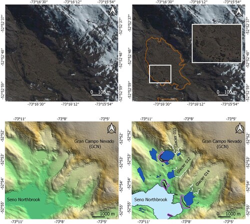
Figure 1. Research area and published studies. (a) Study area indicated by box west of the Gran Campo Nevado, located ca. 130 km south of the Campo de Hielo Patagónico Sur. (b) Mapped area includes overlap rectangles of locations studied previously. Solid black symbols correspond to marine sediment records (MSR), hollow symbols indicate lake sediments cores (LS), Biester et al. (2002) utilize peat records (PR), Lamy et al. (2010) include MSR, LS and PR data while Schimpf et al. (2011) use cave and stalagmites samples (CS). Blue squares indicate the closest automatic weather stations.

Read the detailed description of this figure

(a) Regional map of southern tip of Chile showing the location of the study area, delimitated by a black polygon, and the position of four Automatic Weather Stations around it, represented as small blue squares. (a) Long description: Regional map between 50°00′ to 54°00′ southern latitude and 71°30′ and 74°20′ western longitude, at the southern tip of Chile, North sign pointing upward. The bottom side of the image shows the location of the study area bounded by a 5-sided black polygon, just north of the Magellan Strait, with its eastern boundary the Gran Campo Nevado. The image also shows the position of 4 Automatic Weather Stations represented as small blue squares surrounding the study area: one on the East side at the confluence of the Magellan Strait and Pacific Ocean, and the other 3 located towards Northeast of the study area. The Campo de Hielo Patagónico Sur is indicated as reference on the top part of the map; on the bottom part of the map the Muñoz Gamero Peninsula is shown, on which the Gran Campo Nevado is bordering the study area towards East; Seno Skyring, Riesco Island and Seno Otway are found to the East of Gran Campo Nevado. South of the Strait of Magellan, which has a Northwest–Southeast orientation, the Santa Ines Ice Field is indicated, and the Brunswick Peninsula is displayed on the bottom right of the map. (b) Expanded view of the research area showing the location of core samples and the study areas covered by other research projects, within or near the current research area. (b) Long description: Expanded view of the same map between 52° 36′ to 53° 30′ southern latitude and 72° 50′ to 73° 58′ western longitude, showing the study area with a black polygon, inside of which the Beaufort Bay, the Muñoz Gamero Peninsula, the Tamar, Emiliano Figueroa and Providencia islands are displayed. There are seven boxes with different types of borders to indicate the areas covered in the previous studies of Breuer et al. (2013a), Kilian et al. (2007b), and Koch and Kilian (2005). The location of three automatic weather stations (the same stations as in (a)) are also indicated as blue squares. There are specified symbols distributed within or near the study area that correspond to core samples of marine sediment records, lake sediments cores, peat records and cave and stalagmites. The samples are described in the works of Breuer et al. (2013b), Breuer, Kilian, Schörner, et al. (2013), Shiroya et al. (2013), Kilian et al. (2006), Biester et al. (2002), Lamy et al. (2010) and Schimpf et al. (2011). In addition, the location of some places is indicated as a reference: Manuel Rodríguez Island in the extreme Northwest of the map, and from there, from North to South are situated the Strait of Magellan, Desolación Island and Childs Island. Colcolo Bay is shown as a body of water bordering the Southeastern limit of the study area about 35 km south from the highest point of the Gran Campo Nevado.

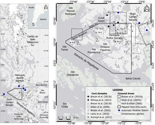
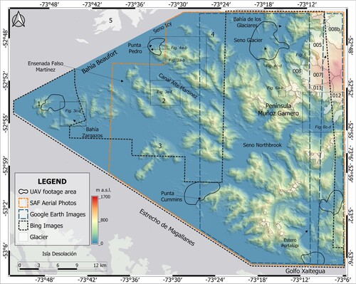
Figure 2. Spatial coverage of imagery used for geomorphological mapping. Planet satellite orthorectified images (Imagery © 2019 Planet Labs Inc.) form the base-map. Mosaics from these satellite images and from Sentinel-2 images cover the entire mapped area so are not indicated. The UAV footage area represents total area visualized during the flight. Colored hillshade of 45° is from ALOS PALSAR DEM and delimits the mapped area. Selected codes from the DGA inventory provided for Gran Campo Nevado glaciers (see Table S1). Islands mentioned in the text are labeled with numbers: 1: Isla Tamar (∼10 km²), 2: Isla Emiliano Figueroa (∼170 km²), 3: Isla Providencia (∼25 km²), 4: Isla Eleodoro (∼8 km²), 5: Isla Merino (∼11 km²).

Read the detailed description of this figure

Study area map with a colored hillshade model (based on ALOS PALSAR DEM), indicating the covered area by the different image sources used to create the geomorphological map. Glaciers are displayed as white polygons, mostly concentrated in the Gran Campo Nevado, at the North-eastern part of the map. Long Description: Map between 52°75′ to 53°15′ southern latitude and 73°54′ to 73°6′ western longitude, North sign pointing upward, showing a colored hillshade model of the study area. The rest of the territory is presented in grayscale. Within the study area, the blue color represents the lowest elevation (sea level) which clearly marks the fjords and bays in the sector. As the elevation increases, the colors change from blue to green, yellow, orange until reaching color red, which represents the highest elevation (1700 m above the sea level), at the North-eastern part of the map, over the Gran Campo Nevado summits. The different image sources used to create the geomorphological map are indicated delimited by polygons with different types of strokes and colors. Ordered by size of area covered in relation to the studied area, from largest to smallest, image sources are indicated as follows: aerial photos from the Aerial Photographic Mapping Service of the Chilean Air Force (SAF), Bing Images, Google Earth images and UAV footage. The glaciers, located in the North-Eastern part of the map, have been represented with white polygons, and identified with the glacier inventory codes from the Chilean Directorate General of Water (DGA); from North to South they are 008b, 005, 007 and 008, 011 and 012. As a reference, Bahía Beaufort, Seno Icy and Bahía de los Glaciares are indicated, limiting the northern margin of the study area, and the Strait of Magellan and Xaltegua Gulf limiting the southern margin. Within the study area, the location of Punta Pedro, Seno Glaciar, Ensenada Falso Martinez, Canal Almirante Martinez and Península Muñoz Gamero are indicated in the northern part; in the southern part, Northbrook Sound, Punta Cummins and Estero Portalupi are shown. In addition, the location of Desolación Island is indicated at the southwestern end of the map, and islands mentioned in the text are labeled with numbers from 1 to 5.

The GCN is located on the Andean cordillera's axis, which is the only continuous orographic barrier between 46 and 56°S, intersecting oceanic as well as meteorological global circulation systems such as the Southern Westerly Winds (Garreaud et al., 2009; Kilian & Lamy, 2012; Lamy et al., 2010). These westerlies have a strong control on local precipitation and temperature patterns (Garreaud et al., 2013) directly impacting geomorphic processes. Precipitation comparisons at 53°S show that precipitation at sea level on the Pacific coast is 59% of the precipitation measured at sea level within the mountains, while to the east, precipitation drastically drops to 25% and 8% at Seno Skyring (to ∼70 km) and Punta Arenas (to ∼150 km), respectively (Schneider et al., 2003; see Figure 1(a)). This barrier leads to high annual precipitation contrasts between >4,000 mm/a over the Pacific, ∼10,000 mm/a in the highly elevated cordillera and <500 mm/a east of the GCN (Möller et al., 2007; Schneider et al., 2003).

Whilst previous research in the study area has focused on the GCN’s glaciology (Davies & Glasser, 2012; Koch & Kilian, 2005; Meier et al., 2018; Möller et al., 2007; Schneider et al., 2007), marine geological mapping efforts to identify submerged glacial landforms (Breuer et al., 2013b; Kilian et al., 2007b), and the extraction of marine, lake and peat sediment records for palaeoclimate reconstructions (Biester et al., 2002; Breuer et al. 2013a; Breuer et al., 2013b; Kilian et al., 2006; Lamy et al., 2010; Shiroya et al., 2013), no comprehensive study of the glacial geomorphology in the fjords and islands west of the GCN has been conducted until present (Figure 1(b)).

In general, there is a lack of glacial geomorphic mapping west of the Andean divide between 44 and 55°S, with the exception of the Gualas, San Rafael, San Tadeo/Quintín (46.4–46.9°S; e.g. Heusser, 1960; Winchester & Harrison, 1996; Glasser et al., 2006; Winchester & Harrison, 1996), the Isla Wellington/Puerto Edén (∼49.1°S; Ashworth et al., 1991) and surrounding the Cordillera Darwin proglacial area (Hall et al., 2013; Izagirre et al., 2018). The limited terrestrial and marine glacial geomorphic data along 1600 km of the Patagonian Ice Sheet’s western margin (see Davies et al., 2020) considerably restricts our understanding of its palaeo-glaciological dynamics, manner of subsequent demise and associated climate feedbacks in the region. We present the first glacial geomorphic map between the GCN and the EDM to address this data gap between 52° and 53°S. This research provides the foundation for future geochronological studies that require a sound knowledge of the glacial geomorphology for targeted sampling. In addition, the methodologies developed here can be used to guide and extend future glacial geomorphic mapping efforts in the Chilean fjords to increase our understanding of Patagonian glacier dynamics along the Pacific coast during the last glacial cycle.

1.1. Study area

The mapped area is delimited by the GCN to the east, Bahia Beaufort and Seno Icy in the N/NW and the EDM in the S/SW, covering an area of 1,565 km² (Figures 1 and 2). The landscape is characterized by deeply incised fjords and islands. The highest peaks in the field area are protruding the GCN up to 1500 m a.s.l. Fjord depths range between ∼700 m NE of Isla Tamar in Bahía Beaufort (Breuer et al., 2013b) and up to ∼1,100 m south of Punta Cummings in the EDM (SHOA, 1998; see Figure 2). There are multiple small islands (<1 km²) in the study area and 10 larger than 1 km². There are four main islands ranging between 8 and 172 km² in size (Figure 2). The Islands are named Emiliano Figueroa, Providencia, Tamar and Eleodoro, and account for 32% of the field area, while the rest is mainland.

The study area was covered by the Patagonian Ice Sheet during the last glacial cycle (see Davies et al., 2020). Though there are no published terrestrial glacial geochronological datasets available to determine deglaciation rates, the marine transgression at 14,000 yr BP in the western Strait of Magellan (Kilian et al., 2007a) and identification of the Mount Burney Tephra (4150 yr BP) in the northern sections of Canal Sweet (Figure 1(b); see Breuer et al. 2013a) indicates that the last deglaciation of the study area occurred between the end of the last glacial and likely finished by the mid-Holocene.

2. Map production

2.1. Imagery

The glacial geomorphic map was produced using remote sensing data, field observations and published bathymetry data (see Figure 2, Table 1; see Breuer et al., 2013a and supplemental material). Mapping was conducted manually and without automatic mapping procedures utilizing QGIS 3.28. Remote sensing data include optical and radiometric data sources which were integrated and manipulated in the GIS environment. In total, 19 optical high-resolution Planet satellite orthorectified images (PI; Imagery © 2019 Planet Labs Inc.) taken between 2017 and 2019 were used, as well as two Sentinel-2 satellite images (SI; 2018, bands 8-11-4 & 8-4-3, see also supplemental material), and 26 aerial photographs at 1:60,000 scale taken by the Servicio Aerofotogramétrico de Chile (SAF; flights in 1978 and 1982). Data from the Advanced Land Observing Satellite Digital Elevation Model (ALOS DEM; 12.5 m e.r.) was used as the topographic base and to map landforms and sediment deposits in excess of 500 meters. To improve landform delimitations, high-resolution images from the 3D Google Earth Pro software Version 7.0 (GE-v7.0) and very high-resolution Bing images (BI), available through the QGIS OpenLayers plugin, were used where images were freely available (Figure 2). The mapped landforms in GE-v7.0 and BI were recognized and mapped onto the planet satellite images (PSI), which has an orthorectified pixel size of three meters and forms the base for the entire map. The aerial photographs were analyzed using traditional stereoscopy and georeferenced to the PIs using a mean of 72 control points per photograph (see supplementary material for detailed methodology).

Table 1. Remote sensing data used.

Data set	Acquisition date	Spatial Resolution (m)	Quantity
Planet satellite images	2017–2019	3	19
Sentinel 2 satellite images	20/10/2018	10 (bands: RGB, NIR)	2
SAF aerial photos	1978–1982	1–1.2; scale 1:60.000	26
ALOS PALSAR DEM	10-06-2015	12.5	1
Maxar Technologies 2019 (Google Earth)	10-10-2004	sub metric	-
Digital Globe 2019 (Bing Map)	No information	sub metric	-

The respective areal cover of each product is shown in Figure 2.

2.2. Field observations

Selected remotely mapped sites were visited during the #ChileFjords18 cruise in November 2018 to corroborate mapped features using direct field measurements, photography and unmanned aerial vehicle footage (UAV: DJI Mavic PRO 4 K HD; Figure 2; see the main map for flight route details). The use of a non-tripulated tool and the high-resolution field photographs and videos obtained from the UAV footage were used in two ways: (1) to observe areas of restricted access, and (2) to capture different angles of landforms between 1 m and ∼1 km² (e.g. Figures 3 and 4(c,d)).

Figure 3. Examples of erosional landforms mapped (see Figures 1 and 2 for location): (a) Hillshade from ALOS PALSAR DEM illuminated from northwest showing glacial cirques in the area close to Punta Pedro. (b) Map of coalescing cirques and arêtes, with a tarn at the base of the most north-eastern cirque. Lakes are shown in blue. (c) Infrared Sentinel image showing eroded bedrock as a gray surface. (d) Interpreted whalebacks (continuous line) and roche moutonnées (dashed line). Ice flow from east to west, selected landform long profiles shown in meters (not to scale). Profiles 1 and 2 show asymmetric cross profile with smooth stoss and steep lee side, whilst profile 3 is symmetric. (e) Planet image showing the clearest asymmetric roche moutonnée example in Falso Martinez Valley. (f) Same location as image 3e with hillshade. Ice flow from SE to NW, long profile of rouche moutonnée plotted in meters (not to scale).

Read the detailed description of this figure

(a) Gray hillshade model, illuminated from the Northwest, in the sector between Punta Pedro and Almirante Martinez Channel, where a topographic high is located. Long Description: Gray hillshade model illuminated from the Northwest, between ∼52°48′ to ∼52°52′ southern latitude and ∼73°26′ to ∼73°34′ western longitude. Punta Pedro is indicated at the northwestern end, and the Almirante Martinez Channel (which has a Northwest– Southeast orientation) is located in the bottom section of the image. Between Punta Pedro and Canal Alte Martinez a topographic high is located, which is part of the western end of Península Muñoz Gamero. (b) Fig 3a interpreted, indicating the presence of five glacial cirques as orange line and several lakes as blue polygons. (c) Infrared satellite image in the Bahía Zargazos sector. The sea is shown in black color, red color highlights the vegetation cover and eroded bedrock devoid of vegetation is shown in gray color at Peninsula Tamar. (d) Image from (c) interpreted, showing whalebacks with NW–SE orientation, Roche Moutonnées with NW–SE to W–E orientation, and several lakes as blue polygons. In addition, the topographic profiles of two whalebacks and one roche moutonnée are displayed. (d) Long Description: Same base image as (c) with geomorphic interpretation. Lakes indicated with blue polygons, majority of lakes (n = 14 of 18) east of 73°44 west. Three whalebacks with Northwest–Southeast orientation indicated with continuous line. Three roche moutonnées with orientation Northwest–Southeast to West–East indicated by dashed line. Above with interpretation, indicating the distribution of lakes (blue polygons), interpreted whalebacks (continuous line) and roche moutonnées (dashed line). In addition, three white graphics show the topographic profiles of two whalebacks and one roche moutonne, showing the pronounced stoss side of the latter. (e) Planet image in natural color of the Almirante Martinez Channel and Emiliano Figueroa island, where water bodies are observed in black color, polished rock in brown color, vegetation in green color and snow in white color. (f) Image from (e) used with a translucent gray hillshade model draped on top to accentuate the relief. One roche mouteéne with a NW–SE orientation with the a-axis indicated by a dashed line. A topographic profile shows the asymmetric shape of the landform with the stoss side facing in Northwest.

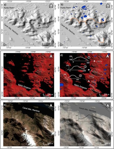
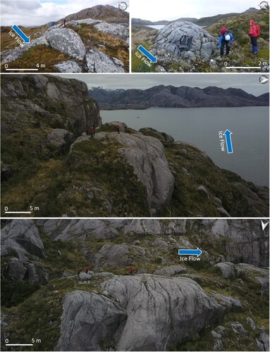
Figure 4. Examples of whalebacks mapped in the field (see Figure 2 for locations). (a) Micro-scale whaleback at Seno Icy. (b) Micro-scale fractured whaleback at Isla Tamar. (c,d) Back and side view of a meso-scale whaleback colonized by vegetation on its stoss side, image captured during a UAV flight at Seno Glaciar.

Read the detailed description of this figure

(a) It shows a whaleback landform in the center of the image, and in the background, there are two researchers. North points to the upper left of the image, and an ice flow direction arrow is pointing to the South. (b) There is a small lake in the background, and in the foreground, there is a cracked front of a well-rounded whaleback. On the right side of the whaleback there are two researchers for scale. North arrow points to the left and the ice flow arrow points to the South West. (c) View from back of a larger whaleback (meso-scale) with investigators standing on it. A steeper landscape with subvertical rock walls of approximately 15–20 m is shown in the background while on the right, a part of a fjord at Seno Glaciar is shown. Ice flow arrow is pointing to the West. (d) View from North of the same whaleback (meso-scale) in (c). Three investigators are standing on it next to erratic boulders on top of the whaleback. Ice flow arrow is pointing to the West.

3. Glacial landform and sediment description

In this section, we describe landform and sediment accumulations associated with (de)glaciation. All of the mapped landforms, commonly meso-scale (1 m–2 km), are listed and defined in Table 2 with corresponding shape files provided as supplemental material. The high-resolution remote sensing data facilitated the identification of landforms with a minimum size of ∼30 m. Glacial erosional landforms and depositional landforms and sediment deposits cover an area of 77% and 23%, respectively.

Table 2. Identification criteria for landforms mapped from satellite/aerial imagery.

Item	Morphology	Identification Criteria	Preferred recognition tool	Glaciological significance	Uncertainties/confusion
Glacier landforms & sediment
Cirques	Wide amphitheater-shaped pots on mountain flanks or embedded in plateau edges. Shows abrupt boundaries with the surrounding terrain.	Semicircular shapes limited by steep slopes. Shaded by changes in height or relative relief. The base of the cirques may have color variations with respect to the surrounding environment. It generally contains a lake (Tarn) at its base.	Best in APs > Hillshade and slope maps from DEM > GI > BI, PSI, SI.	Indicates the presence of restricted or localized mountain glaciation. Allows palaeo glacier equilibrium line altitudes (ELA) calculations.	Hardly likely to confuse.
U-shaped valley	Wide valleys with a U-shaped cross-sectional profile.	Wide valley limited by steep sloping walls. In the area often forming fjords.	APs > Hillshade from DEM > BI, GI, SI, PSI.	Indicates direction of glacier flow and ice discharging corridors.	Hardly likely to confuse.
Scarps	Marks the upper limit of abrupt steps on slopes.	Upper limit of steep slope greater than 60° in a rock face, often smooth (abraded) with channels orthogonal or semi-orthogonal to the slope.	Hillshade and slope maps from DEM, APs > GI.	Indicate glacial erosion or basal weakening on rocky slopes.	Possible confusion with fault scarps.
Ice-scoured bedrock	Large exposed bedrock or lightly vegetated surface with numerous small lake basins and glacial erosional features at every scale.	Gray to light pink colors when vegetation is present. Geological structures are present. Exposed surface has a rough and irregular texture and often contains attributes elongated in the direction of the ice direction (mounds).	BI > GI > PSI, APs, SI.	Evidence of large areas covered by ancient glaciers at basal melting point.	Possible underestimation of areal cover where bedrock is obscured by vegetation.
Whaleback	Features parallel to the ice flow direction, formed by glacial erosion. Form of elongated hills with similar slopes.	In the bedrock, it is observed as a change in the structure of the surface. Often with smooth surfaces from glacial abrasion. Often in groups. Difficult to distinguish individually at DEM scale.	APs >> Hillshade from DEM. Contours can guide > GI, SI (IR). Checked with Profile Tool when possible.	It shows the direction of ice flow and can indicate former glacier basal conditions.	In a DEM, it can be confused with a roche moutonnée. Confusion can be reduced when using APs.
Roche moutonnée	Features parallel to the ice flow direction, formed by glacial erosion. Elongated hill shape with asymmetrical slopes with a steep, plucked lee side.	In the bedrock, it is observed as a change in the structure of the surface. Often with smooth surfaces on the stoss side from glacial abrasion. The down glacier side (lee) has a steep slope and absent rocky material. Often in groups. Difficult to distinguish individually at DEM scale.	APs >> Hillshade from DEM. Contours can guide > GI, SI (IR). Checked with Profile Tool when possible.	It shows the ice flow direction, and can indicate former glacier basal conditions.	In a DEM, it can be confused with whalebacks. Confusion can be reduced when using APs.
Glacial drift	Irregular cover of unconsolidated material forming flat deposits	In high-resolution images, it is observed as accumulations of heterogeneously sized sediment. They often occur on the fringes of glaciers and / or affected by gravitational processes.	BI > GI > APs	Ancient ice presence	Possible confusion with mass movement deposits.
Kettle kame topography (KKT)	Large belts consisting of disorganized hills and hollows.	It is observed as smooth textured surfaces by sedimentary coverage with pockmarked appearance often containing a pond. KKT can contain ridges.	APs, GI, PSI, BI.	May indicate ice stagnation, wastage, ice-block meltout or results of GLOF events.	Possible confusion with Knock and Lochan topography when the rock surfaces are colonized by vegetation.
Moraine complex	Simple or multiple mounds of positive relief. It can be linear, curved, sinuous or toothed seen in planar view. Commonly showing an asymmetric transversal profile.	Changes in relief imprint shading. If the mound is colonized by vegetation, it may show color changes. On both sides of the relief, light and dark tones are opposed.	APs >> Hillshade maps from DEM when possible for resolution, GI, SI.	Marks a former stagnation position of a glacial lobe.	Possible confusion with modeled rock promontory when the latter is covered by vegetation. Ridges and shorelines could potentially be confused.
Outwash plains	Flat sediment accumulation on the valley floor. Commonly dissected by a twisted hydrographic pattern.	They are observed as flat surfaces at the bottom of the valleys, with gray tones due to the presence of sediments and soft texture, only disturbed by numerous sinuous channels commonly darker in tone.	APs, BI > GI, PSI > SI	Marks the main drainage routes for glacial meltwater and other glacier-fed streams.	Possible confusion with delta, alluvial plain or ice-contact deposits.
GLOF Deposits	Glacial lake outburst floods (GLOF) are a type of mass movement (e.g. mud flow) deposit with heterogeneous sediment size. Related spatially with contemporary glacier and/or breached moraines.	Discordant in color and texture with surrounding. Gray color is common. Position related to contemporary glaciers/lake/moraine is evident.	APs, BI, GI > PSI	Bursting of glacial lakes and consequent flooding of proglacial environment.	Difficult to confuse with other sedimentary deposits due to position and connectivity with morphogenetic agent.
Hydrological features
Contemporary glaciers	Bare ice, snow, debris and surface structures (crevasses and seracs).	White to light blue colors. Smooth to rough surface. Debris appears gray to black. Abrupt transition with other terrain.	Is clear in all data. Limits improve with resolution.	Current icefield discharge route.	Snow/debris cover boundary difficult to decipher, otherwise not difficult to identify.
Rivers and streams	Channels of water draining a valley.	Colors vary from blue to black, with sharp boundaries with surrounding terrain (5); white in AP is also possible.	BI, GI > APs, PSI > SI	Indicate contemporary drainage routes and may be sourced from modern glaciers.	Possible to confuse with narrow channels without contemporary drainage.
Meltwater channels	Channels often not contain current drainage. Channels can follow or cut along local slopes. On steep slopes are straight.	Well-defined edges and steep boundaries with the surrounding terrain. Shadowing due to change in height or relative relief. The bottom of the channel can present colors different from those of the surroundings. Generally sinuous in low gradient terrain and with snow/water when are close to active glaciers.	APs, BI, GI > PSI	They indicate high volumes of melt water production. They can indicate the position of old ice margins especially when seen in association with moraines or outwash plains sandur.	Possible to confuse with contemporary drainage.
Water bodies	Freshwater bodies within enclosed basins.	Blue, black or white in color imagery, typically elliptical o rounded in shape. Black and clearly observed in infrared SI images (bodies >800 m^2). Sharp boundaries with terrain.	BI, APs > GI, PSI, SI	Impeded drainage. Can result from rock basins formed by glacial over deepening. Useful to recognize kettle and kame topography.	Areas in the shadow of high relative relief. Size are very variable but is difficult to confuse with other landforms.
Non-glacial geomorphology
Marine terraces	Rocky promontory with flat surfaces commonly close to and parallel to current shore line. In some sectors they may be limited by cliffs	In DEM and APs are flat rocky surfaces often interrupted by fractures. In satellite images, natural color, are commonly reflective (rocky) and gray in color. Usually surrounded by water and parallel to shore line.	APs, BI, GI > PSI, SI > hillshade from DEM	Could be used to estimate glacial isostatic rebound rates and sea level variations.	Possible to confuse with flat bedrock surfaces scoured by glacier ice.
Aluvial deposits (fan, delta and plains)	Landforms typically feed by streams. Fans are sub-horizontal fan shaped on valley sides. Plains are sub-horizontal deposits filling valley bottom and deltas and occur in contact with water bodies.	Accumulation with abrupt limits with surrounding terrain due to changes in the vegetation cover. Commonly with patterns of braided streams on the surface. Gray or green colors for forest coverage are common. Shape allows to distinguish between fan / delta and plains. Profiles on GE or views on APs allow seeing longitudinal profile.	APs, GE Boundaries also on BI, PSI.	Reworking of unconsolidated material by contemporary fluvial channels and streams.	Possible to misinterpret as fossil delta or ice contact deposit or with outwash plains.
Landslides (falls and flows)	Sedimentary deposits not related to continuous water runoff or ice. Falls typically form irregular accumulations with heterogeneous sediment size. When related to channels are fan shape.	Accumulations with diffuse contacts in case of falls, sometimes gradual. Differences in texture respect to surrounding in both falls and flow are clear. Observed better in colored high-resolution images as spotted texture (falls).	APs, GE Boundaries also on BI, PSI.	May indicate rework of unconsolidated material deposited on unstable slopes	It is possible to misinterpret falls as glacial drift and flows as alluvial deposits.
Other sedimentary deposits	Deposits related to water bodies. Marginal lake and beach. Peat bogs are also included	Flat surfaces next to water bodies and sharp limit with surrounding, are soft in texture and gray to pale rose in color.	BI, GE, APs, PSI	Sedimentary structural and geochronological studies on sediments	Possible confusion with alluvial plains.
Geological elements
Geological contact	Plane representing the surface limiting two different types of rocks. From surface, it is observed as a line.	In the study area and available images, the granitoids show a clear whitish color and are roughly textured, contrasting with the dark gray colors and softer texture of the older mafic rocks.	BI, GE, APs, PSI + terrain observation	Lithology can exert control in glacial landform distribution.	Possible to confuse with changes in surfaces rock characteristics due to other factors such as surface erosion or sediment deposits.

Table and definitions have been extracted and modified from Glasser and Jansson (2008), Glasser et al. (2005), Darvill et al. (2014), Davies and Glasser (2012) and Izagirre et al. (2018). Preferred recognition tool acronyms are DEM: Alos Palsar Digital Elevation Model, GI: Google Earth Images (GE-v7.0), BI, Bing Satellite Images; PSI, Planet Satellite Images; SI, Sentinel 2 Satellite Images and APs represent traditional aerial pair stereographic analysis.

3.1. Glacial erosional landforms

A total of 463 meso-scale landforms related to glacial erosion were identified and mapped with criteria detailed in Table 2.

3.2. Cirques

In total, 70 armchair-shaped hollows with steep sides and back walls were identified in the study area and interpreted as cirques (Figure 3(b) and main map). The majority of cirques or cirque clusters are located proximal to the GCN. The number of cirques reduces significantly westward likely as a function of lower elevation (Figure 3(a,b)). The base of ice-free cirques ranges in altitude from 32 to 539 m a.s.l. with a mean base altitude of ∼270 m a.s.l. While 52% of ice-free cirques show a clear south-facing aspect, the remainder have no preferred aspect direction. Cirques developed facing westward or eastward are rare (<7%).

3.2.1. U-shaped valleys

Macro to micro-scale negative relief created by glacial erosional action is visible on remote sensing images in form of U-shaped valleys. Twenty-eight valleys with a clear U-shape transversal profile were mapped. These range from 0.5 to 8.3 km in length with preferred direction toward NW (azimuth 290°), in agreement with the principal structural geology in the area (NW/SE; Breuer et al., 2013b). U-shaped valley widths range from 100 to 600 m.

3.2.2. Areal scouring

Areal scouring refers to areas of ice-scoured bedrock with undulating positive and negative relief. Areal scouring can feature an assemblage of streamlined bedrock features (whalebacks), stoss and lee forms (e.g. roches moutonnées) and rock basins (Rea & Evans, 1996). About 30% of the total ice-free land mapped corresponds to ice-scoured bedrock. In the study area, regions of scoured bedrock often include rocky basins containing shallow ponds or marshes in the hollows, with whalebacks and roches moutonnées separating them.

3.2.3. Whalebacks

Whalebacks are positive relief landforms produced in the subglacial environment and were principally identified using aerial photographs and during field work (Table 2). They are defined as bedrock knolls that have been smoothed and rounded on all sides by glacier ice (Glasser & Bennett, 2004). Whalebacks represent 78% of all mapped positive eroded landforms (n = 51) in the study area. Their mean perimeter polygon altitude, i.e. the base is at 126 m a.s.l., but they have been mapped up to an elevation of 669 m a.s.l. The whalebacks a-axes range between 200 and 2,300 m in length. During fieldwork whalebacks of >10 m in length were identified (Figure 4).

3.2.4. Roches moutonnées

Roches Moutonnées are positive relief landforms with a pronounced asymmetric longitudinal profile, abraded slope on the stoss side and a plucked lee side indicating glacier flow direction (Glasser & Bennett, 2004). This clear asymmetry is not easily visible on the DEM (Figure 3(d)), with confidence reached only with landforms exceeding ∼600 m in length (Figure 3(f)). In contrast, with the AP stereoscopic analysis, it is possible to identify and map roches moutonnées a-axes from ∼150 m in length. When APs were unavailable (see Figure 2), we use the BI to determine whether the stoss side was abraded or plucked. A total of eighteen roches mountonées were identified between 53 and 344 m a.s.l. and the mean base altitude is 136 m a.s.l.

3.2.5. Micro-features

Glacial striations are produced by entrained subglacial sediment abrading bedrock. Chatter marks are crescentic-shaped gauges, formed by rock fragments being dragged across subglacial bedrock. Both erosional micro-features were identified in the field at elevations up to 700 m a.s.l.

3.3. Glacial depositional landforms and sediment

Glacial depositional landforms are scarce in the study area (22%). Undifferentiated glacial drift is common over bare rock and spatially related to modern glacial activity (total area coverage: 1.28 km², see Figures 5 and 6(d)). In total, 128 glacial depositional landforms and sediment accumulations were identified and mapped (Table 2; Map).

Figure 5. Bing Satellite Image (2019) over ALOS PALSAR DEM view in 3D, east of Seno Glaciar. The terminus of glacier 007 is at ∼160 m a.s.l. (DEM elevation). Glacial meltwater is actively flowing 600 m down valley before producing a well-developed outwash plane. Northeast of Glacier 007, a frozen lake is at ∼485 m a.s.l. and a GLOF deposit is located downhill. Scoured bedrock is observed as gray polished surfaces in the whole area.

Read the detailed description of this figure

Digital elevation model over a very high-quality image from Bing Satellite Image, indicating a GLOF deposit downstream from a frozen lake in the upper part of the mountain, and an outwash plain 600 m downstream from the Glacier 007. Long Description: Digital elevation model over a very high-quality image from Bing Satellite Image showing a mountainous relief with steep slopes and grayish rocky outcrops; the base is limited by an extension to the East of Seno Glaciar and the summits are covered with snow. North points to the left with an inclination of about 30° downwards. A Frozen Lake is indicated in the upper left part of the image, Glacier 007 in the upper right part descending towards the viewer, a GLOF deposit in the bottom-left quadrant near the East extension of Seno Glaciar, and an outwash plain in the bottom-right quadrant, 600 m downstream of Glacier 007.

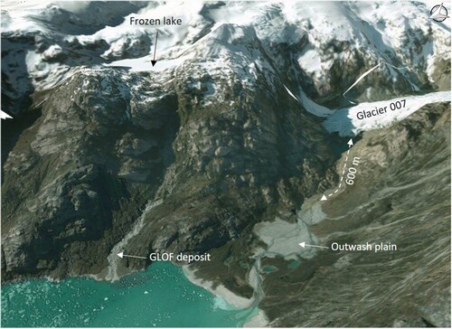
Figure 6. Examples of depositional landforms. (a) High-resolution GI image north of Seno Northbrook showing spotted deposits. (b) PI image showing same site as (a) with area of kettle kame topography delimited (full line). (c) Hillshade from DEM ALOS PALSAR illuminated from 45°, south–west GCN (see Figure 2 for location). (d) Mapping output of (c) site. Moraine area indicated with purple hollow polygons, respective moraine crests in black lines. More than one crest inside a polygon indicates a moraine complex. Lakes in blue and glacier margins in stippled white line (see Table S1).

Read the detailed description of this figure

(a) High-resolution Google image showing a mountainous relief in dark brown tones, partially covered by snow from the NW–SE diagonal of the image frame to the North. (b) Image from (a) interpreted, where a kettle kame topography has been delimited with an irregular polygon. There is an auxiliary image showing an enlarged view of the southwest part of the landform. (c) Hillshade model of the sector between Gran Campo Nevado and Seno Northbrook. The relief color changes with elevation, from light green tones at sea level to brownish (∼600 m a.s.l.) and gray tones in the higher sectors (∼1000 m a.s.l.). (d) Image from (c) interpreted, indicating the distribution of three glaciers at the foot of the Gran Campo Nevado. In the margins of glaciers are located proglacial lakes limited by moraine areas. Two moraines border to the southwest with the Seno Northbrook. (d) Long Description: Image from (c) interpreted, where polygons have been drawn to indicate the distribution of Seno Northbrook (light blue-fill), five lakes (blue-fill; three of which are proglacial lakes), Moraine area (2 transparent polygons with purple borders and moraine ridges indicated by black lines) and the glacier margins (stippled white lines). From top to bottom the glaciers are identified with codes 011, 012 and 014. Streamlined landforms are indicated by a continuous blue line in the SW of the study area.

3.3.1. Moraines

Ice marginal moraines are ridges formed at the lateral and/or frontal margin of glaciers, typically with asymmetric profiles (Benn & Evans, 2010; Table 2). The moraines are composed of glacial till ranging between silt to boulder-sized rounded to very angular sediments. We distinguish individual moraine crests from the entire moraine complex, the latter can include more than one moraine crest. In our map, the moraine complex area and moraine crests are represented by polygons and lines, respectively (Figure 6(d)). In total, 118 individual terrestrial and seven submarine moraine crests were mapped, corresponding to seventy-one moraine complexes. The majority of moraine crests/complexes cover a small area (5,400 – 400,000 m²) with a relative relief of 7–80 m between the crest and the surrounding topography. In general, the moraines crests/complexes are located in one of two locations: (I) between 2 and 10 km from ice-free cirques, with a relief of <20 m and emerging from the fjords; (II) ∼1 km down-valley from active glacier margins, located between 30 and 420 m a.s.l. with a relief of 30–60 m (e.g. moraines located in the three glacial valleys SW of the GCN; Figures 2 and 6(c,d)).

3.3.2. Kettle kame topography (KKT)

KKT is generated through supraglacial or ice-contact glaciofluvial sediment deposition around in-situ ice, wastage and ice-block melt out (Gordon & Mcewen, 1993) or following GLOF events (Iribarren et al., 2015). As the ice melts over time, a pitted topography remains. Twenty-eight KKT areas have been mapped (Figure 6(a,b)) and are dispersed across the study area. The KKTs are located between 20 and 511 m a.s.l. and cover an area of 0.01–1.52 km².

3.3.3. Outwash plains

Outwash plains are relatively flat deposits at the valley base composed of sub-rounded to rounded sediment and dissected by active/inactive fluvial processes (Table 2). A total of four outwash plains were identified. Three have active proglacial meltwater channels from GCN glaciers (Figure 5). One outwash plain is located ca. 2 km from the current glacier 008 margin, indicating a former glacial still-stand down-valley, which represents the ice limit in 1942 AD (Kilian et al., 2007b).

4. Hydrological features

4.1. Contemporary glaciers

Present-day glaciers were mapped using the National Glacier Inventory of Chile as a reference (DGA, 2014). The glacier names used in the map follow the DGA numbering, excluding their shared first eight-digit prefix code CL112422 (e.g. CL112422005 = Glacier 005). Table S1 lists the glacier names used here with those from other glacier inventories. The boundaries have been updated with Sentinel 2 (IR band combination of 2017) and PSI from 2018 (Table 1). In total, 54 glaciers were mapped with surface areas ranging from 0.02 to 22.83 km².

4.2. Fluvial channels

We differentiate fluvial channels as active or inactive according to the surface runoff observed in the remote sensing images.

4.2.1. Active rivers and streams

Present-day river activity was inferred from the images covering 2018–2019 (Table 1). Flowing water with no glacial source was considered as active and defined as river or stream depending on their respective widths (n = 1456).

4.2.2. Meltwater channels

Meltwater channels are active channels formed in the proglacial area by glacial meltwater (e.g. Izagirre et al., 2018; Lovell et al., 2011), of which 271 were identified in the study area.

4.3. Water bodies

We mapped 1637 fresh water bodies in the study area (Table 2), ranging from 3 to 2750 m², of which 47 correspond to bedrock-floored tarns.

5. Non-glacial landforms and sediment

Several non-glacial landforms and sediment accumulations were mapped for completeness and are provided in the final map. Items mapped are marine terraces, alluvial deposits (Gutiérrez-Elorza, 2008), landslides (Hungr et al., 2014) and peat bogs. More detailed differentiation of non-glacial deposits is beyond the scope of this work.

6. Geology

We provide the only geological map available of the study area as a shape file in the supplemental materials (scale: 1:1,000,0000; SERNAGEOMIN, 2003). It is outwith the scope of this paper to create a more detailed geological map. The local geology is dominated by Cretacious intrusives, mainly tonalites, diorites and granodiorites. Jurassic-Cretacious mafic complexes outcrop locally (see supplemental material). The principal structural control in the area corresponds to the NW/SE Magallanes–Fagnano lateral slip fault system which controls the common structural lineaments’ orientation (Breuer et al., 2007b). Observations in the field and remote sensing analysis were used to establish a better overlap and relationship between the local geology and the glacial landforms discussed.

7. Discussion

In terms of methodology where precise changes in the relief needed to be identified (e.g. discriminating between whalebacks and roches mountonnées), the DEM and 3D visor GE-v7.0 were used together (Table 1). However, when comparing the output to aerial photograph (AP) stereographic analysis, it became clear that the DEM and 3D GE visor overestimate the number of whalebacks and underestimated the number of roches moutonnées in the study area. The resolution of the DEM and 3D GE visor hampers the clear discrimination between both landforms; thus, only through the use of the APs could landforms be accurately mapped. We also used the very high-resolution BI images (Table 1) to discriminate if the stoss side looked abraded (smooth) or plucked (high presence of fractures and shadows, and lack of detrital material). This is a time-consuming method but produces higher confidence in landform discrimination and final geomorphic map output.

From our map, it is clear that the peninsulas and islands located between the GCN and the EDM have been impacted by late Pleistocene glacial expansion and recession to varying degrees. Glacial erosional landforms account for 78% of all mapped features. From micro-scale striations and chatter marks to meso-scale whalebacks and roches moutonnées to macro-scale aerial scouring of bedrock, the occurrence of these features indicates efficient subglacial erosion due to warm-based, debris loaded, potentially fast-flowing ice. Glacier retreat was likely rapid and continuous due to a relative lack of marine and terrestrial depositional landforms marking glacier stabilization (28× kame and kettle topography, 71× moraine complex, 5× outwash plains; see Map).

Meso-scale glacial erosional landforms in the study area are dominated by whalebacks (74%) and roches moutonnées (26%). Krabbendam and Glasser (2011) suggest that lithology (hardness) and joint spacing exerts a strong control on the distribution of whalebacks and roches moutonnées. In our study area, 67% of whalebacks and 67% of roches moutonnées occur on harder intrusive granitoids and 33% of each landform on softer mafic rocks. The lack of lithological preference for either landform suggests that lithology does not exert a strong control on landform distribution in the fjords of southwestern Chile. To investigate the influence of joint spacing on landform distribution requires a more detailed analysis of the structural geology and paleo-channel distribution, which is beyond the scope of this work.

The distribution of whalebacks and roches mountonnées may represent different subglacial conditions. Whalebacks are generally associated with warm-based thicker ice, low sliding velocities and available basal meltwater, whereas roches moutonnées preferentially form underneath warm-based thin fast-flowing ice (Hallet, 1996), with abundant subglacial meltwater (Glasser & Bennett, 2004). Whalebacks were mapped up to 700 m a.s.l. whilst roches moutonnées were only identified up to 344 m a.s.l. We hypothesis that each landform is associated with a different glacier flow regime, either during the same or multiple glacial cycles. Whalebacks were likely produced when ice cover in the fjords was more extensive, i.e. thicker, whilst the roches moutonnées were formed during phases of thinner ice. Such thinner ice likely occupied the area during the last glacial to de-glacial transition, potentially exacerbated by the de-glacial marine transgression (∼14 ka BP; Kilian et al., 2007a), leading to potentially thinner fast-flowing outlet glaciers from the Patagonian Ice Sheet.

8. Conclusions

• We present the first terrestrial glacial geomorphic map between the Gran Campo Nevado and EDM (52° to 53°S), to address the data gap in reconstructing Patagonian Ice Sheet dynamics west of the Cordillera de los Andes in southwestern Patagonia.

• All features were mapped manually without automatic mapping procedures, eliminating the errors related to automation and increasing our mapping accuracy using a number of different remote sensing products.

• In total 4290 individual features were mapped in the study area (1565 km²) of which 862 are directly related to glacial activity. The most relevant are:125 terrestrial and submarine moraine crests, 71 moraine complexes, 70 cirques, 51 whalebacks, 40 scarps, 28 kettle kame topography, 28 U-shaped valleys and 18 roches moutonnées,

• The spatial distribution of whalebacks and roches moutonnées indicates a lack of lithological control on their formation, which may alternatively be related to glacier bed conditions and/or joint spacing.

• Glacial erosional landforms dominate over depositional landforms indicating a warm-based, sediment laden and meltwater-rich subglacial environment. In addition, the occurrence of whalebacks and roches moutonnées suggests a dynamic and changing ice velocity and thickness regime during Patagonian Ice Sheet cover and retreat.

Software

We use Sentinel Application Platform (SNAP, v.5.0) by ESA to work with Sentinel data sets. Google Earth Pro 7.3.2 (©2019 Google LLC) was useful to observe different perspectives of landforms. Finally, all mapping and data manipulation were conducted in the Open Source Geospatial Foundation Project software QGIS 3.280 [https://qgis.org] while the final map design was improved in Adobe Illustrator (AI).

Open scholarship

This article has earned the Center for Open Science badge for Open Data. The data are openly accessible at http://dx.doi.org/10.5525/gla.researchdata.1384

Acknowledgements

Special thanks go out to Captain Hugo Cardenas and the entire Mary Paz II crew for making nearly everything possible, Juan-Carlos Aravena and Marcelo Arevalo for logistical support at Universidad de Magallanes and in Punta Arenas, and everyone who helped during fieldwork preparations in Santiago and Punta Arenas. We would also like to thank the thorough and thoughtful comments provided by reviewers Federico Ponce, Andy Hein, Thomas Pingle and associate editor Jasper Knight which considerably improved the manuscript.

Disclosure statement

No potential conflict of interest was reported by the author(s).

Data availability statement

The data that support the findings of this study are available from the Glasgow University online repository at the following link: https://dx.doi.org/10.5525/gla.researchdata.1384. The primary data has the following license: CC-BY-SA. See supplemental materials for further information.

Correction Statement

This article has been corrected with minor changes. These changes do not impact the academic content of the article.

Additional information

Funding

This study was supported by research grants from the Royal Geographical Society with IBG, British Society for Geomorphology, Quaternary Research Association, FONDECYT [grant number 3170869], and a Hanse-Wissenschaftskolleg Institute for Advanced Studies Junior Fellowship awarded to A.J.G.; FONDECYT [grant number 1161110] of J-L.G & A.J.G.; University of Liverpool Early Career Researchers Grant awarded to R.K.S. We would like to thank AMG Group for sponsoring field gear for the #ChileFjords18 expedition.

References

- Ashworth, A. C., Markgraf, V., & Villagran, C. (1991). Late quaternary climatic history of the Chilean channels based on fossil pollen and beetle analyses, with an analysis of the modern vegetation and pollen rain. Journal of Quaternary Science, 6(4), 279–291. https://doi.org/10.1002/jqs.3390060403
- Bendle, J. M., Thorndycraft, V. R., & Palmer, A. P. (2017). The glacial geomorphology of the lago Buenos Aires and Lago Pueyrredón ice lobes of central Patagonia. Journal of Maps, 13(2), 654–673. https://doi.org/10.1080/17445647.2017.1351908
- Benn, D. I., & Evans, D. J. A. (2010). Glaciers and glaciation (pp. 802). Hodder Education.
- Biester, H., Kilian, R., Franzen, C., Woda, C., Mangini, A., & Schöler, H. F. (2002). Elevated mercury accumulation in a peat bog of the Magellanic Moorlands, Chile (53 S) – an anthropogenic signal from the southern hemisphere. Earth and Planetary Science Letters, 201(3–4), 609–620. https://doi.org/10.1016/S0012-821X(02)00734-3
- Blomdin, R. (2012). The late glacial history of the Magellan strait in Southern Patagonia, Chile: Testing the applicability of KF-IRSL dating [MSc. Thesis], Stockholm University. urn:nbn:se:su:diva-137807.
- Breuer, S., Kilian, R., Baeza, O., Lamy, F., & Arz, H. (2013a). Holocene denudation rates from the superhumid southernmost Chilean Patagonian Andes (53 S) deduced from lake sediment budgets. Geomorphology, 187, 135–152. https://doi.org/10.1016/j.geomorph.2013.01.009
- Breuer, S., Kilian, R., Schörner, D., Weinrebe, W., Behrmann, J., & Baeza, O. (2013b). Glacial and tectonic control on fjord morphology and sediment deposition in the Magellan region (53 S), Chile. Marine Geology, 346, 31–46. https://doi.org/10.1016/j.margeo.2013.07.015
- Caldenius, C. C. Z. (1932). Las glaciaciones cuaternarias en la Patagonia y tierra del fuego: Una investigación regional, estratigráfica y geocronológica.—Una comparación con la escala geocronológica sueca. Geografiska Annaler, 14(1–2), 1–164. http://repositorio.segemar.gov.ar/308849217/860.
- Clapperton, C. M., Sugden, D. E., Kaufman, D. S., & McCulloch, R. D. (1995). The last glaciation in central Magellan strait. Southermost Chile. Quaternary Research, 44(2), 133–148. https://doi.org/10.1006/qres.1995.1058
- Clapperton, C. M. (1983). The glaciation of the Andes. Quaternary Science Reviews, 2(2–3), 83–155. https://doi.org/10.1016/0277-3791(83)90005-7
- Clapperton, C. M. (1992). La última glaciación y deglaciación en el estrecho de magallanes: Implicaciones para el poblamiento de tierra del fuego. Anales del Instituto de la Patagonia, 21, 113–128. http://bibliotecadigital.umag.cl/handle/20.500.11893/1002.
- Clark, P. U., Dyke, A. S., Shakun, J. D., Carlson, A. E., Clark, J., Wohlfarth, B., Mitrovica, J. X., Hostetler, S. W., & McCabe, A. M. (2009). The last glacial maximum. Science, 325(5941), 710–714. https://doi.org/10.1126/science.1172873
- Darvill, C. M., Bentley, M. J., Stokes, C. R., Hein, A. S., & Rodés, Á. (2015). Extensive MIS 3 glaciation in southernmost Patagonia revealed by cosmogenic nuclide dating of outwash sediments. Earth and Planetary Science Letters, 429, 157–169. https://doi.org/10.1016/j.epsl.2015.07.030
- Darvill, C. M., Stokes, C. R., Bentley, M. J., & Lovell, H. (2014). A glacial geomorphological map of the southernmost ice lobes of Patagonia: the Bahía Inútil–San Sebastián, Magellan, Otway, Skyring and Río Gallegos lobes. Journal of Maps, 10(3), 500–520. https://doi.org/10.1080/17445647.2014.890134
- Davies, B. J., Darvill, C. M., Lovell, H., Bendle, J. M., Dowdeswell, J. A., Fabel, D., Garcia, J.-L., Geiger, A., Glasser, N. F., Gheorghiu, D. M., Harrison, S., Hein, A. S., Kaplan, M. R., Martin, J. R. V., Mendelova, M., Palmer, A., Pelto, M., Rodés, A., Sagredo, E. A., … Thorndycraft, V. R. (2020). The evolution of the Patagonian Ice Sheet from 35 ka to the present day (PATICE). Earth-Science Reviews, 204, 103152. https://doi.org/10.1016/j.earscirev.2020.103152
- Davies, B. J., & Glasser, N. F. (2012). Accelerating shrinkage of Patagonian glaciers from the little Ice Age (∼AD 1870) to 2011. Journal of Glaciology, 58(212), 1063–1084. https://doi.org/10.3189/2012JoG12J026
- DGA. (2014). Catastro nacional de glaciares. Unidad de Glaciología y Nieves, Dirección General de Aguas. Ministerio de Obras Públicas, información entregada por Ley de Transparencia, febrero 2014.
- García, J.-L., Hein, A. S., Binnie, S. A., Gómez, G. A., González, M. A., & Dunai, T. J. (2018). The MIS 3 maximum of the Torres Del Paine and Última esperanza ice lobes in Patagonia and the pacing of southern mountain glaciation. Quaternary Science Reviews, 185, 9–26. https://doi.org/10.1016/j.quascirev.2018.01.013
- García, J.-L., Kaplan, M. R., Hall, B. L., Schaefer, J. M., Vega, R. M., Schwartz, R., & Finkel, R. (2012). Glacier expansion in southern Patagonia throughout the Antarctic cold reversal. Geology, 40(9), 859–862. https://doi.org/10.1130/G33164.1
- Garreaud, R., Lopez, P., Minvielle, M., & Rojas, M. (2013). Large-scale control on the Patagonian climate. Journal of Climate, 26(1), 215–230. https://doi.org/10.1175/JCLI-D-12-00001.1
- Garreaud, R. D., Vuille, M., Compagnucci, R., & Marengo, J. (2009). Present-day South American climate. Palaeogeography, Palaeoclimatology, Palaeoecology, 281(3–4), 180–195. https://doi.org/10.1016/j.palaeo.2007.10.032
- Geiger, A. J. (2015). Patagonian glacial reconstructions at 49° S. PhD. Thesis, University of Glasgow. http://theses.gla.ac.uk/6404/
- Glasser, N., & Jansson, K. (2008). The glacial map of Southern South America. Journal of Maps, 4(1), 175–196. https://doi.org/10.4113/jom.2008.1020
- Glasser, N. F., & Bennett, M. R. (2004). Glacial erosional landforms: Origins and significance for palaeoglaciology. Progress in Physical Geography, 28(1), 43–75. https://doi.org/10.1191/0309133304pp401ra
- Glasser, N. F., Jansson, K., Mitchell, W. A., & Harrison, S. (2006). The geomorphology and sedimentology of the ‘témpanos’ moraine at Laguna San Rafael, Chile. Journal of Quaternary Science, 21(6), 629–643. https://doi.org/10.1002/jqs.1002.
- Glasser, N. F., Jansson, K. N., Goodfellow, B. W., De Angelis, H., Rodnight, H., & Rood, D. H. (2011). Cosmogenic nuclide exposure ages for moraines in the Lago San Martin Valley, Argentina. Quaternary Research, 75(3), 636–646. https://doi.org/10.1016/j.yqres.2010.11.005
- Glasser, N. F., Jansson, K. N., Harrison, S., & Rivera, A. (2005). Geomorphological evidence for variations of the north Patagonian icefield during the holocene. Geomorphology, 71(3), 263–277. https://doi.org/10.1016/j.geomorph.2005.02.003
- GLIMS & NSIDC. (2005, updated 2018). Global land ice measurements from space glacier database. Compiled and made available by the international GLIMS community and the National Snow and Ice Data Center, Boulder, CO, USA. https://doi.org/10.7265/N5V98602
- Gordon, J., & Mcewen, L. (1993). Quaternary of Scotland (J. Gordon & D. Sutherlands, pp. 499–501). London: Joint Nature Conservation Committee, Chapman and Hall. https://doi.org/10.1007/978-94-011-1500-1_1.
- Gutiérrez-Elorza, M. (2008). Geomorfología (pp. 920). Spain: Pearson/Prentice Hall. ISBN: 978-84-8322-389-5.
- Hall, B. L., Porter, C. T., Denton, G. H., Lowell, T. V., & Bromley, G. R. (2013). Extensive recession of Cordillera Darwin glaciers in southernmost South America during Heinrich Stadial 1. Quaternary Science Reviews, 62, 49–55. https://doi.org/10.1016/j.quascirev.2012.11.026
- Hallet, B. (1996). Glacial quarrying: A simple theoretical model. Annals of Glaciology, 22, 1–8. https://doi.org/10.3189/1996AoG22-1-1-8
- Hein, A. S., Hulton, N. R., Dunai, T. J., Schnabel, C., Kaplan, M. R., Naylor, M., & Xu, S. (2009). Middle pleistocene glaciation in Patagonia dated by cosmogenic-nuclide measurements on outwash gravels. Earth and Planetary Science Letters, 286(1–2), 184–197. https://doi.org/10.1016/j.epsl.2009.06.026
- Heusser, C. J. (1960). Late-Pleistocene environments of the Laguna de San Rafael area, Chile. Geographical Review, 50(4), 555–577. https://doi.org/10.2307/212310
- Hughes, P. D., Gibbard, P. L., & Ehlers, J. (2013). Timing of glaciation during the last glacial cycle: Evaluating the concept of a global ‘last glacial maximum’ (LGM). Earth-Science Reviews, 125, 171–198. https://doi.org/10.1016/j.earscirev.2013.07.003
- Hulton, N. R., Purves, R. S., McCulloch, R. D., Sugden, D. E., & Bentley, M. J. (2002). The last glacial maximum and deglaciation in Southern South America. Quaternary Science Reviews, 21(1), 233–241. https://doi.org/10.1016/S0277-3791(01)00103-2
- Hungr, O., Leroueil, S., & Picarelli, L. (2014). The Varnes classification of landslide types, an update. Landslides, 11(2), 167–194. https://doi.org/10.1007/s10346-013-0436-y
- Iribarren, P., Mackintosh, A., & Norton, K. (2015). Reconstruction of a glacial lake outburst flood (GLOF) in the Engaño Valley, Chilean Patagonia: Lessons for GLOF risk management. Science of The Total Environment, 527-528, 1–11. https://doi.org/10.1016/j.scitotenv.2015.04.096
- Izagirre, E., Darvill, C. M., Rada, C., & Aravena, J. C. (2018). Glacial geomorphology of the Marinelli and Pigafetta glaciers, Cordillera Darwin Icefield, southernmost Chile. Journal of Maps, 14(2), 269–281. https://doi.org/10.1080/17445647.2018.1462264
- Kilian, R., Baeza, O., Steinke, T., Arevalo, M., Rios, C., & Schneider, C. (2007a). Late pleistocene to holocene marine transgression and thermohaline control on sediment transport in the western Magellanes Fjord system of Chile (53 S). Quaternary International, 161(1), 90–107. https://doi.org/10.1016/j.quaint.2006.10.043
- Kilian, R., Biester, H., Behrmann, J., Baeza, O., Fesq-Martin, M., Hohner, M., Schimpf, D., Friedmann, A., & Mangini, A. (2006). Millennium-scale volcanic impact on a superhumid and pristine ecosystem. Geology, 34(8), 609–612. https://doi.org/10.1130/G22605.1
- Kilian, R., & Lamy, F. (2012). A review of glacial and holocene paleoclimate records from southernmost Patagonia (49–55 S). Quaternary Science Reviews, 53, 1–23. https://doi.org/10.1016/j.quascirev.2012.07.017
- Kilian, R., Schneider, C., Koch, J., Fesq-Martin, M., Biester, H., Casassa, G., Arévalo, M., Wendt, G., Baeza, O., & Behrmann, J. (2007b). Palaeoecological constraints on late glacial and holocene ice retreat in the southern Andes (53°S). Mass Balance of Andean Glaciers, 59(1), 49–66. https://doi.org/10.1016/j.gloplacha.2006.11.034
- Koch, J., & Kilian, R. (2005). ‘Little Ice age’ glacier fluctuations, Gran Campo Nevado, southernmost Chile. The Holocene, 15(1), 20–28. https://doi.org/10.1191/0959683605hl780rp
- Krabbendam, M., & Glasser, N. F. (2011). Glacial erosion and bedrock properties in NW Scotland: Abrasion and plucking, hardness and joint spacing. Geomorphology, 130(3–4), 374–383. https://doi.org/10.1016/j.geomorph.2011.04.022
- Lamy, F., Kilian, R., Arz, H. W., Francois, J.-P., Kaiser, J., Prange, M., & Steinke, T. (2010). Holocene changes in the position and intensity of the southern westerly wind belt. Nature Geoscience, 3(10), 695–699. https://doi.org/10.1038/ngeo959
- Lovell, H., Stokes, C. R., & Bentley, M. J. (2011). A glacial geomorphological map of the seno skyring-seno otway-strait of Magellan region, southernmost Patagonia. Journal of Maps, 7(1), 318–339. https://doi.org/10.4113/jom.2011.1156
- McCulloch, R. D., Fogwill, C. J., Sugden, D. E., Bentley, M. J., & Kubik, P. W. (2005). Chronology of the last glaciation in central strait of Magellan and Bahía Inútil, southernmost South America. Geografiska Annaler: Series A, Physical Geography, 87(2), 289–312. https://doi.org/10.1111/j.0435-3676.2005.00260.x
- Meier, W. J.-H., Grießinger, J., Hochreuther, P., & Braun, M. H. (2018). An updated multi-temporal glacier inventory for the Patagonian Andes with changes between the little Ice Age and 2016. Frontiers in Earth Science, 6, 62. https://doi.org/10.3389/feart.2018.00062
- Mendelová, M., Hein, A. S., Rodés, Á, & Xu, S. (2020). Extensive mountain glaciation in central Patagonia during marine isotope stage 5. Quaternary Science Reviews, 227, 105996. https://doi.org/10.1016/j.quascirev.2019.105996
- Möller, M., Schneider, C., & Kilian, R. (2007). Glacier change and climate forcing in recent decades at gran campo nevado, southernmost Patagonia. Annals of Glaciology, 46, 136–144. https://doi.org/10.3189/172756407782871530
- Rea, B. R., & Evans, D. J. (1996). Landscapes of areal scouring in NW Scotland. Scottish Geographical Magazine, 112(1), 47–50. https://doi.org/10.1080/00369229618736977
- Sagredo, E. A., Moreno, P. I., Villa-Martínez, R., Kaplan, M. R., Kubik, P. W., & Stern, C. R. (2011). Fluctuations of the Última esperanza ice lobe (52 S), Chilean Patagonia, during the last glacial maximum and termination 1. Geomorphology, 125(1), 92–108. https://doi.org/10.1016/j.geomorph.2010.09.007
- Schimpf, D., Kilian, R., Kronz, A., Simon, K., Spötl, C., Wörner, G., Deininger, M., & Mangini, A. (2011). The significance of chemical, isotopic, and detrital components in three coeval stalagmites from the superhumid southernmost Andes (53°S) as high-resolution palaeo-climate proxies. Quaternary Science Reviews, 30(3-4), 443–459. http://doi.org/10.1016/j.quascirev.2010.12.006
- Schneider, C., Glaser, M., Kilian, R., Santana, A., Butorovic, N., & Casassa, G. (2003). Weather observations across the southern Andes at 53 S. Physical Geography, 24(2), 97–119. https://doi.org/10.2747/0272-3646.24.2.97
- Schneider, C., Schnirch, M., Acuña, C., Casassa, G., & Kilian, R. (2007). Glacier inventory of the Gran Campo Nevado ice cap in the southern Andes and glacier changes observed during recent decades. Global and Planetary Change, 59(1), 87–100. https://doi.org/10.1016/j.gloplacha.2006.11.023
- SERNAGEOMIN. (2003). Mapa Geológico de Chile: Versión digital. Servicio Nacional de Geología y Minería, Publicación Geológica Digital, No. 4 (CD-ROM, versión1.0, 2003). Santiago.
- Shiroya, K., Yokoyama, Y., Obrochta, S., Harada, N., Miyairi, Y., & Matsuzaki, H. (2013). Melting history of the Patagonian Ice Sheet during termination I inferred from marine sediments. Geochemical Journal, 47(2), 107–117. https://doi.org/10.2343/geochemj.2.0231
- SHOA. (1998). Golfo Xaultegua Estrecho de Magallanes/[material cartográfico]: por el Servicio Hidrográfico y Oceanográfico de la Armada de Chile. Valparaíso: Servicio Hidrográfico y Oceanográfico de la Armada de Chile, diciembre 1998. 1 mapa: color; 69 ( 103 cm en hoja 75 ( 109 cm. http://www.bibliotecanacionaldigital.gob.cl/bnd/631/w3-article-320538.html
- Soteres, R. L., Peltier, C., Kaplan, M. R., & Sagredo, E. A. (2020). Glacial geomorphology of the strait of Magellan ice lobe, southernmost Patagonia, South America. Journal of Maps, 16(2), 299–312. https://doi.org/10.1080/17445647.2020.173617
- Winchester, V., & Harrison, S. (1996). Recent oscillations of the San Quintin and San Rafael glaciers, Patagonian Chile. Geografiska Annaler: Series A, Physical Geography, 78(1), 35–49. https://doi.org/10.1080/04353676.1996.11880450