Harmonizing multi-source backscatter data using bulk shift approaches to generate regional seabed maps: Bay of Fundy, Canada

ABSTRACT

Advances in sonar technology have revolutionized our ability to map the seafloor, however, differences between legacy and modern data pose challenges when analysing multi-source datasets. Acoustic backscatter recorded via multibeam echosounder is commonly used to characterize the seafloor, but a lack of standardized calibration often yields relative rather than absolute backscatter measurements, hindering comparison between surveys. ‘Bulk shift’ methods have been developed for harmonizing legacy backscatter datasets using overlapping survey areas for relative statistical calibration. This becomes increasingly difficult, though, given many datasets collected over extensive time periods. Backscatter data were collected in the Bay of Fundy, Canada, using multiple sonar systems and vessels over an 18-year period. Here, we propose a reproduceable strategy for harmonizing this large volume of disparate backscatter data using the bulk shift method. A final, harmonized map is presented for the entire Bay of Fundy and is validated using in situ observations from seafloor imagery.

KEYWORDS:

• Backscatter
• multibeam echosounder
• seabed mapping
• backscatter calibration
• bulk shift harmonization
• benthic

1. Introduction

Backscatter data collected by bathymetric sonars indicate the acoustic reflectivity of the seafloor, which has become an important data source for seabed mapping. Because seafloor backscatter depends partially on the properties of the substrate, it can be used as a proxy in benthic ecology research – for example, to inform on the distribution of sediment types (De Falco et al., 2010; Fonseca & Mayer, 2007; Lamarche et al., 2011) or benthic habitats (Brown et al., 2012; Che Hasan et al., 2012; Ierodiaconou et al., 2018). Multibeam echosounders (MBES) facilitate the efficient acquisition of backscatter data. While single-beam sonars ensonify a single location beneath the vessel, MBES map a broad swath across-track, often many times wider than the water depth. For this reason, MBES are increasingly preferred for a wide range of seabed mapping applications (Brown & Blondel, 2009).

Although the use of MBES backscatter has become commonplace for seabed mapping, a variety of factors hinder direct comparison between different backscatter datasets. MBES system calibration is not universally adopted (Lamarche & Lurton, 2018), meaning that backscatter is often measured on a relative, rather than absolute, dB scale (Rice & Cooper, 2015). Relative backscatter can still provide useful information on the seabed for a variety of mapping purposes (Lucieer et al., 2018), but is often specific to a single sonar system or survey. The frequency at which the sonar operates may also influence the measured backscatter, even for calibrated systems (Lurton, 2010). This occurs due to factors that are difficult to constrain, such as the effects of seafloor roughness and sediment heterogeneity on scattering of the acoustic signal for different sonar frequencies and beam configurations (Hughes Clarke et al., 2008), or from differences in substrate penetration and reflectivity intensities in stratified substrates (Weber & Lurton, 2015). Finally, relative backscatter values can even differ depending on data processing methods, such as selection of software or processing parameters (Malik et al., 2019), which may be difficult to adjust for processed legacy data. Lacking stringent absolute calibration procedures and consistent operating parameters, these combined factors are likely to render multi-source MBES backscatter datasets inconsistent regarding the substrate properties of interest for seabed mapping applications (Lamarche & Lurton, 2018).

‘Bulk shift’ or ‘offset’ approaches have been proposed as a method for integrating multi-source backscatter data for seabed mapping applications, wherein a single continuous map layer is desirable (Hughes Clarke et al., 2008; Misiuk et al., 2020). Broadly, this refers to the systematic adjustment of relative dB values in order to standardize multiple backscatter datasets. The approach suggested by Misiuk et al. (2020) proposes to use areas of mutual coverage between surveys in order to model the bulk shift empirically as a function of the observed error between backscatter datasets. Conceptually, this is a form of relative empirical backscatter calibration (Rice & Cooper, 2015), which enables outputting a single backscatter mosaic that is the union of multiple individual datasets. Hereafter, we refer to the relative calibration and combination of multiple disparate datasets as ‘harmonization’. Because bulk shift models are derived from pre-existing backscatter mosaics, raw data and acoustic processing software are not required to produce a harmonized dataset, making this approach potentially useful for integrating legacy backscatter data with modern analyses. Such approaches have shown promise for harmonizing backscatter datasets collected using a single sonar model, but at different time intervals and operating frequencies (Misiuk et al., 2020), and also for broad scale habitat mapping with several pre-existing backscatter mosaics (Misiuk et al., 2021).

Regional seabed mapping efforts stand to benefit immensely from harmonized backscatter products that match the extent of regional bathymetric maps (e.g. tens of thousands of km²), which include heterogeneous seafloor habitats but lack important sedimentary information (e.g. sediment composition, grain size). Regional backscatter products act as important predictors of seafloor sediment properties for habitat mapping efforts, but their availability remains scarce compared to bathymetric data. Over large geographic areas, particularly those with complex seafloor topography (e.g. near the coasts), it is increasingly likely that MBES data are collected over multiple campaigns, by different vessels and sonars, and over extended time periods. These factors all serve to complicate the harmonization of backscatter data. Specifically, we currently lack strategies for (i) simultaneously handling many disparate, partially overlapping datasets, which implies decisions regarding the order in which they are harmonized, and (ii) validating the results of multi-step regional backscatter harmonization. The former is an important consideration for multi-step harmonization because early bulk shift corrections may impact subsequent operations. Independent validation is critical in this context; the validity of a multi-step backscatter harmonization is questionable given the large number of potentially confounding factors that affect multi-source backscatter consistency, such as the use of different operating frequencies and beam widths.

Here, we present efforts to generate a regional harmonized backscatter mosaic comprising a large number of mapping surveys in the Bay of Fundy, Canada, using bulk shift approaches. A strategy is developed for determining the harmonization order, which prioritizes dataset characteristics of similarity and extensiveness. In addition to individual internal bulk shift model evaluations, we present a unified statistical validation for the final backscatter layer using independent data. Finally, the full harmonized backscatter map is presented for the Bay of Fundy.

2. Methods

2.1. Study area

The Bay of Fundy is a highly dynamic and heterogeneous system. Characteristics of the bay have been previously described in detail, including its geology (Fader et al., 1977; Shaw et al., 2012; Wade et al., 1996), physiography (Amos et al., 1980; Todd et al., 2014), and oceanography (Greenberg, 1984; Li et al., 2015; Wu et al., 2011). Briefly, it is a macrotidal estuarine embayment that experiences the largest tides in the world (Amos et al., 1980). The tidal range is greatest towards the head where it may exceed 15 m (Archer & Hubbard, 2003). Counter-clockwise circulation and high mean current velocities > 0.5 ms⁻¹ occur throughout most of the bay, and exceed 5 ms⁻¹ at their most extreme (Li et al., 2015), which has motivated interest in tidal energy at certain locations (Karsten et al., 2008). These conditions drive the constant reworking of post-glacial seabed sediments, which include glacial debris, silt, sand, clay, and sand/gravel surficial geology units (Fader et al., 1977). Glacial landforms are commonly observed on the seabed, including moraines, eskers, and drumlins; other features, including flow-parallel dunes and sand banks, are the product of reworking by waves and currents (Shaw et al., 2012; Todd et al., 2014). Much of the bay is < 100 m in depth, but the deepest areas exceed 230 m toward the mouth (Shaw et al., 2012; Todd et al., 2014).

2.2. Data

MBES data were collected for the entire Bay of Fundy by the Canadian Hydrographic Service (CHS), Geological Survey of Canada (GSC), and University of New Brunswick (UNB) over a period of 18 years (Todd et al., 2011b). Raw MBES data from this collection were reprocessed using commercial software to produce individual backscatter rasters. Corrected backscatter mosaics for each data set were produced using QPS FMGT for all data sets except survey data from 1996 and 1999. Backscatter datagrams for these older MBES data sets were not supported by FMGT and were therefore processed using Caris HIPS and SIPS. All backscatter mosaics were generated at 5 m pixel resolution. Some of the raw MBES data were not available or could not be processed using modern software. At several locations, data from two previous backscatter data compilations that met the criteria for this study (i.e. overlapping other surveys; Hughes Clarke et al., 2008; Todd et al., 2011b) were cropped and included in the set of individual component backscatter rasters.

Processed backscatter mosaics that matched two criteria were selected for this study. First, data from surveys were selected that overlapped with other surveys to facilitate use of the bulk shift methods. Second, where areas have been surveyed multiple times (e.g. by the CCGS Frederick G. Creed in 1992-1994, then again between 1996 and 2008; Hughes Clarke et al., 2008), the more recent of the data were selected. These requirements precluded small sections of the full surveyed area, reducing the overall coverage as compared with prior work utilizing the same datasets (e.g. Hughes Clarke et al., 2008; Todd et al., 2011b), and 13 datasets collected between 1996 and 2008 were retained for this study. Additionally, two pre-processed data compilations were included, comprising data from the CCGS Frederick G. Creed, CSL Plover, and CSL Heron (Table 1 and Figure 1). MBES data were provided in an uncalibrated form, rendering all backscatter measurements relative, rather than absolute. Additionally, a continuous bathymetric surface for the Bay of Fundy was provided by the GSC at 10 m horizontal resolution (Todd et al., 2011a), which was used as an additional predictor variable in the bulk shift models (see section 2.3).

Figure 1. MBES data coverage for individual surveys in the Bay of Fundy, Canada. Each colour group represents surveys collected by the same vessel, with different shades representing various years. Note that CSL Plover/CSL Heron data were obtained as a combined pre-processed grid. A more comprehensive list of individual backscatter mosaic coverages and their respective survey year is provided in the Main Map.

A regional map of the Bay of Fundy, Canada, overlain by multibeam echosounder survey coverages. There are 15 individual backscatter mosaics. Mosaics collected by the same survey vessel share the same colour but have different shades representing varying survey years.

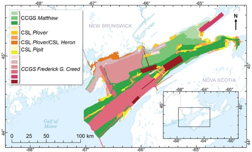
Table 1. Summary of surveys and multibeam echosounders used to collect data that were reprocessed and used in this study (Hughes Clarke et al., 2008; Parrot et al., 2010a, 2010b, 2010c, 2010d, 2010e; Parrott et al., 2013; Todd et al., 2011b).

Vessel	Survey years	Sonar model	Operating frequency (kHz)
CCGS Frederick G. Creed	1996, 1999	EM1000	95
CCGS Frederick G. Creed	2006, 2007, 2008	EM1002	93/98
CCGS Matthew	2007, 2008, 2009	EM710	71-97
CSL Heron	2006, 2007	EM3002	300
CSL Plover	2007, 2008, 2009	EM3002	300
CSL Pipit	2007, 2008	EM3002	300

Ground truth video observations of seabed substrates were used for validating the harmonized backscatter mosaic. Drop camera videos were collected between 2017 and 2019 in order to ground truth a benthic habitat map across the extent of the bay (Wilson et al., 2021). Video drifts were conducted at 281 sites over a distance of ∼100-500 m across a range of environments. Ten still images were extracted from each drift to describe the substrate texture (according to Wentworth, 1922) and dominant epifauna. Observations of substrate texture and dominant epifauna were summarized to produce seven seabed classes that were encountered consistently throughout the bay, and which could be readily differentiated from each other. Each of 1879 images from 190 of the 281 sample sites was assigned to a seabed class; a detailed description of the dataset and methods is provided by Wilson et al. (2021). Here, the images at each sample station were aggregated to their geographic mean centre (i.e. their average x- and y- coordinates) and assigned a label based on the majority of seabed classes observed, producing $n=190$ independent ground-truth observations corresponding to the number of sites for which the seabed was classified. Backscatter values were extracted at each ground-truth site before and after harmonization for each dataset.

Benthic Hamon grab samples were also collected at 23 targeted locations in 2019 to characterize the infauna and sediment grain size. A subsample of the sediments from each grab was analysed for particle grain size composition. The volume of grain size data was not sufficient for quantitative validation of the harmonized backscatter mosaic, but was used for qualitative evaluation and comparison with results from the video observations (Main Map).

2.3. Backscatter harmonization

All raster grids were resampled and aligned prior to harmonization. The 2008 CCGS Matthew backscatter dataset was extensive and consistent over a large part of the bay; all other backscatter data were resampled and aligned with this grid at 5 m resolution, then coarsened to 50 m using a mean aggregation. This ensured the co-location of backscatter measurements per grid cell, but also decreased the computational requirements for modelling relative calibrations between datasets. A reduction in resolution may also facilitate the bulk shift to some degree by reducing fine scale differences in backscatter response between sonar units over such a large area.

The bulk shift method was implemented following Misiuk et al. (2020) using the 50 m backscatter grids. This process begins by extracting co-located backscatter measurements for two datasets at areas where raster cells overlap. Then, by treating one dataset as the reference, or ‘target’, and one as the ‘shift’, which will undergo correction, the error is calculated between backscatter measurements, and is used to apply bulk corrections to the entire ‘shift’ dataset. Specifically, this was implemented as a series of four steps: (i) scatterplots of the error were visualized to assess whether it is consistent, or whether it varies according to backscatter or depth values; (ii) an empirical model is fit to predict the error as a function of the ‘shift’ backscatter values and/or the water depth; (iii) the error model is used to predict a correction offset for the entire ‘shift’ dataset; and (iv) the corrected ‘shift’ layer is mosaicked with the ‘target’ to produce a single backscatter layer. Following these steps, the quality of the error model was assessed by calculating the mean absolute error (MAE), Kolmogorov–Smirnov (K–S) statistic, probability density function (PDF), and cumulative distribution function (CDF) between the ‘target’ and ‘shift’ datasets, before and after correction. A package for performing the bulk shift in the R programming language is hosted online (https://github.com/benjaminmisiuk/bulkshift).

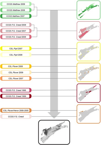
Where more than two datasets overlap simultaneously, it is necessary to determine an order in which to apply the bulk shifts. These decisions may be important; a multi-step bulk shift procedure implies that early corrections could affect subsequent operations. In order to minimize these effects, the order in which datasets were combined was determined by a set of criteria. First, where possible, all surveys conducted using a single vessel and MBES system were combined to produce harmonized mosaics. This was expected to introduce the least possible amount of error into the broader analysis, given that a single MBES system is more likely to operate using similar parameters over multiple surveys (particularly, the operating frequency). Having combined surveys conducted using a single vessel and system, the most extensive of those mosaics were combined. This decision was based on maximizing the area and diversity of seabed that was used to inform bulk shifts over the largest part of the study area. Finally, isolated surveys remaining at the periphery of the study area, portions of the previous harmonized layer (Hughes Clarke et al., 2008) for which raw data were unavailable, and the lowest quality legacy datasets (e.g. from 1996, 1999) were integrated. Either intercept-only (i.e. ‘mean’) or linear regression error models were selected based on the quality of fit as estimated using the evaluation statistics (but see the Results section for two exceptions). Where similar fits were observed, the simpler model was preferred. The specific order of operations is indicated in Figure 2.

Figure 2. Summary of the multi-step bulk shift process used to create the final harmonized backscatter map for the Bay of Fundy. More comprehensive details on the harmonization order and model information for each bulk shift used to produce the harmonized backscatter mosaic can be found in the Supplementary Material S2.

A flow diagram summarizing the order in which individual mosaics were harmonized to create the final backscatter mosaic. The more extensive mosaics which were collected using the same survey vessel were harmonized first, followed by less extensive and isolated mosaics.

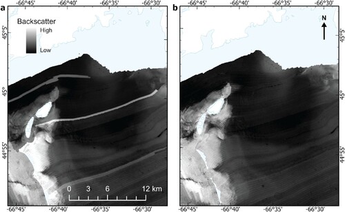
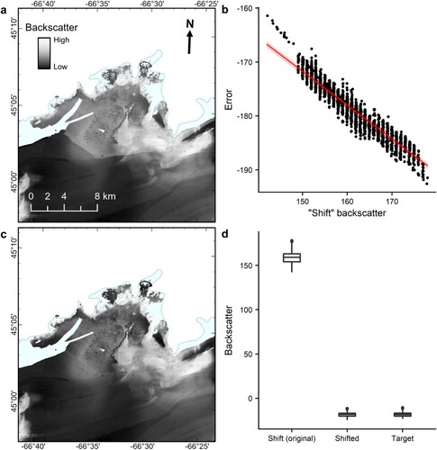
A modified bulk shift procedure was also applied at some locations to improve non-random localized data artefacts – for example, where backscatter values for a single acquisition line were offset from adjacent lines due to changes in acquisition settings (Hughes Clarke et al., 2008). This can be highly useful for areas where erroneous backscatter data may affect subsequent bulk shift models (e.g. Figure 3). First, the backscatter mosaic was cropped to isolate the incorrect data. Bulk shift methods normally rely on overlapping data to derive relative statistical calibrations; inverse distance weighting (IDW) was therefore used to interpolate the coverage of the mosaic over the cropped area by several raster cells to generate a small, synthetic area of overlap. This overlap was then used to re-calibrate the isolated incorrect data with respect to the surrounding backscatter values using a simple bulk shift model, whereby the corrected values replace both the original and interpolated data. This is based on the expectation that proximal backscatter values provide a useful estimate that may be used to re-calibrate the obviously incorrect data, while leaving relative backscatter differences within the area generally unaffected (e.g. Figure 3(b)). Evaluation statistics between the interpolated ‘target’ and ‘shift’ data are calculated as described previously.

Figure 3. Line artefacts present in the CCGS Frederick G. Creed (a) were corrected using a modified bulk shift approach to produce a corrected mosaic (b).

A side-by-side comparison of backscatter mosaics before and after correcting line artefacts present within the datasets. Figure A on the left showcases three line artefacts present within various datasets where the raster cells have backscatter values that are higher than the surrounding cells. The right image, representing the post-harmonization results, has no obvious remnants of the line artefacts and the larger mosaic remained unaffected.

2.4. Validation

A key assumption of the bulk shift method is that the backscatter signals from separate datasets are each dependent on similar seabed properties that influence acoustic reflectivity. Systematic differences between backscatter intensities recorded by different echosounders over variable substrate types would invalidate bulk shift models, as the substrate is essentially being used for relative calibration (Misiuk et al., 2020). This issue may be mitigated somewhat by the data resolution (50 m), which serves to generalize the acoustic response of the seabed over a broad area. Regardless, the assumption that each backscatter dataset responds consistently to the same substrate properties cannot be taken for granted here given the large number of datasets and the range of frequencies at which they were collected. This assumption must be validated empirically.

We tested the null hypotheses that, for each seabed class observed in the ground-truth video samples, backscatter does not differ between survey datasets. This is motivated by the expectation that if the bulk shift harmonization was successful, individual survey datasets should not be distinguishable based on the distribution of backscatter values for a given set of similar seabed samples. Significantly different backscatter measurements between surveys for a given seabed class may indicate a poor harmonization that is not suitable for subsequent use (e.g. as a surrogate for substrate properties). One-way randomization ANOVA tests were applied to test this hypothesis. This method of testing is a preferential alternative to less powerful nonparametric tests when the assumptions for the classic parametric ANOVA are not met. For this test, data variance between groups (here, individual surveys) is compared to variance within groups by deriving a pseudo F-ratio: (1) $\begin{array}{c}F={\displaystyle \frac{VA{R}_b}{VA{R}_w},}\end{array}$(1) where (2) $\begin{array}{c}VA{R}_b=\sum _{i=1}^K{\displaystyle \frac{n_i{({\overline{Y}}_i-\overline{Y})}^2}{K-1},}\end{array}$(2) (3) $\begin{array}{c}VA{R}_w=\sum _{i=1}^K\sum _{j=1}^{n_i}{\displaystyle \frac{{(y_{ij}-{\overline{Y}}_i)}^2}{N-K},}\end{array}$(3) and $n_i$ is the number of observations in group $i$, ${\overline{Y}}_i$ is the within-group mean, $\overline{Y}$ is the mean of all samples, $K$ is the total number of groups, $N$ is the total number of observations, and $y_{ij}$ is observation $j$ of group $i$. Here, there is no minimum total number of observations $n_i$ per group, nor is there a minimum number of samples per group for each individual seabed class.

In the context of this study, the F-statistic becomes larger with increasing backscatter similarity within a dataset and decreasing similarity between datasets for a given seabed class. Significance of the statistic can be determined by permuting the dataset labels (i.e. randomly assigning the observed backscatter values to the datasets) and calculating $F$ via Equation (1) to obtain $F^{\pi }$. By iterating the permutations many times (here, $10,000$), we can tally the number of times that $F>F^{\pi }$ and divide by the number of iterations to obtain an estimate of the probability that the difference in backscatter between groups is greater than to be expected by random chance (e.g. at the $\alpha =0.05$ level). One-way randomization ANOVA tests were run for each seabed class in R (R Core Team, 2019) to test whether backscatter values differed between surveys both prior to and after harmonization using the bulk shift.

3. Results

3.1. Backscatter harmonization

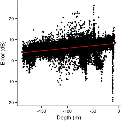
The choice of error model for the bulk shift corresponded to differences between vessel and MBES systems, and therefore, also the order in which the data were combined. Model statistics suggested that an intercept-only (i.e. ‘mean’) error model performed comparably to regression with more parameters for datasets collected using the same vessel and sonar; it was selected for all same-system inter-year corrections (e.g. Figure 4). The selection of intercept-only models at the first phase of bulk shift corrections precludes issues of increasingly large predicted errors outside the range of sampled values that may affect subsequent harmonization operations. Having combined data collected using a single sonar and vessel where feasible, linear regression with a bathymetric covariate was selected in the majority of remaining cases. Similar to previous findings, linear relationships were observed between the backscatter error and water depth for datasets collected using different MBES units (Misiuk et al., 2021; Figure 5). In two cases, non-parametric models (boosted regression trees; BRT) were selected to handle isolated cases of obvious non-linear error between backscatter datasets (Supplementary material S2), which occurred, for example, as a function of the frequency response of disparate sediment types (Hughes Clarke et al., 2008), or due to apparent insufficient angular compensation for legacy data that could not be reprocessed here (e.g. 1999 CCGS Frederick G. Creed data).

Figure 4. An intercept-only (i.e. ‘mean’) error model was used for harmonizing all same-system corrections such as the 2008 and 2009 CCGS Matthew data shown here. Backscatter measurements for two datasets are extracted at areas where raster cells overlap (a). Then, the mean backscatter error is calculated between datasets and is used to apply bulk corrections to the ‘shift’ dataset to produce a continuous mosaic (b).

A side-by-side comparison of backscatter mosaics before and after applying a bulk shift correction using an intercept-only error model. The bulk shift harmonization method uses the area of overlap between two layers for relative statistical calibration. Image A on the left highlights this area of overlap in red. Image B on the right shows the post-harmonization results, and visually appears to be a continuous backscatter layer with no obvious divisions between the two original layers.

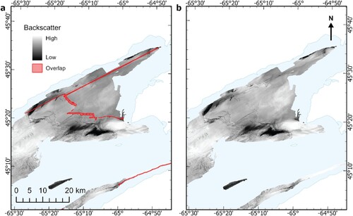
Figure 5. Linear relationship between depth and backscatter error ($\mathrm{slope}=0.02$dB/m) for the Pipit 2007 data, compared to the combined CCGS Frederick G. Creed/Matthew data.

A scatterplot depicting a positive linear relationship between depth and backscatter error values for two datasets.

In all cases, the mean absolute error (MAE) between backscatter rasters was < 2 dB after bulk shifting (Supplementary material S2). The lowest errors (MAE < 1 dB) generally occurred when combining datasets that used the same, or similar, MBES models (e.g. 93/98 kHz EM1002 and 71–97 kHz EM710), and also where backscatter data were incorporated from a previous harmonized mosaic (Hughes Clarke et al., 2008; Todd et al., 2011b; Figure 6). Because the latter were scaled in arbitrary units (0–255), these bulk shift operations also comprised linear rescaling by the regression error models. The error was comparatively elevated where MBES systems differed more substantially in operating frequency (e.g. 71–97 kHz EM710 and 300 kHz EM3002), yet K-S statistics suggested that the similarity between data distributions were much improved following the bulk shift.

Figure 6. Data from a previous harmonized mosaic (a; Hughes Clarke et al., 2008) were incorporated where legacy data were unavailable. The linear bulk shift error model (b) rescales the data to match the ‘target’, even using values on arbitrary non-dB scales (e.g. 0-255). The regression line indicates the modelled error where the datasets overlap, which also varies as a function of water depth (indicated by the error band). Following correction, the datasets are mosaicked (c), and data distributions are compared between datasets at the area of overlap (d).

Read the detailed description of this figure

Four images including two maps showing two datasets before and after harmonization, along with a scatterplot of the results of the bulk shift error model and a box plot of the data distributions compared between the two. Fig. 6 Long Description: Figure A in the top left (a) is a map showing an example of where data from a previous harmonized mosaic was incorporated where legacy data were unavailable to expand the coverage of the map. Figure B in the top right is a scatter plot which shows the results of the linear bulk shift error model applied to the data and highlights a negative linear relationship. A regression line is plotted with an error band, which indicates the modelled error where the datasets overlap, which also varies as a function of water depth. Figure C in the bottom left is a map of the same two datasets from Figure A after they have been harmonized. Figure B in the bottom right is a boxplot showing the data distributions compared between datasets at the area of overlap.

3.2. Validation

While the backscatter values of three of the observed seabed classes were significantly different between datasets prior to harmonization, we found no significant difference between datasets for any of the seabed classes after bulk shifting (Table 2). From interpretation of $F$ and $p$ statistics, the greatest improvement occurred for ‘Mixed sediments’, for which backscatter values were initially highly dissimilar between datasets ($p=0$), but were indistinguishable by dataset after bulk shifting ($p=0.4321$; Figure 7). Note that original ‘Creed 1999’ values were on a disparate non-dB scale, and were omitted along with the seabed samples from this survey area from randomization ANOVA tests before harmonization, but could be included after bulk shifting (Table 2, Figure 7).

Figure 7. ‘Mixed sediment’ backscatter value distributions for each MBES dataset (a) before and (b) after bulk shift harmonization.

Two boxplots showing the backscatter value distributions for each MBES dataset before and after bulk shift harmonization. The boxplot on the left shows the before results, and the plot on the right shows the after results.

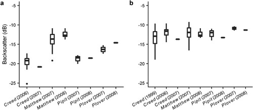
Table 2. Results of one-way randomization ANOVA tests for differences in backscatter between datasets for each seabed class.

Class	Original			Harmonized
	$n$	$F$	$p$	$n$	$F$	$p$
Sand	47	0.9716	0.4748	68	1.7560	0.1049
Gravelly sand	20	3.1466	0.0431*	22	0.7713	0.4845
Mixed sediments	73	34.5805	0*	77	0.9325	0.4344
Tidal scoured mixed sediments	12	3.5411	0.0699	12	0.8949	0.5100
Silty gravel with anemones	15	6.6052	0.0041*	15	1.6008	0.2614
Silt	7	2.0141	0.4012	7	0.2053	0.7372
Bedrock and boulders^†	–	–	–	–	–	–

*Significant at $\alpha =0.05$_.

^† Not enough samples for randomization tests.

4. Discussion

Individual MBES survey datasets for the Bay of Fundy were visually indistinguishable following application of the bulk shift approach (Main Map), as described by Misiuk et al. (2020). Visual interpretability of the final backscatter map layer is useful for understanding the surficial geology of the bay, but efforts to achieve a harmonized mosaic are additionally motivated by the need for seafloor sediment and habitat proxies that may be used for predictive modelling (e.g. Wilson et al., 2021). Whether the final backscatter map product is useful towards these goals may therefore dictate the success of the bulk shift procedure. Independent validation of the final backscatter mosaic here using seafloor imagery suggested that data from multiple surveys were statistically indistinguishable following the bulk shift methodology, according to observed seabed classes. Therefore, we consider the full harmonized backscatter layer fit for use in future modelling activities in the Bay of Fundy. Although internal bulk shift model statistics provide a relative indication of the quality of calibration between individual datasets, we suggest that independent contextual validation is necessary to determine whether such backscatter data products are fit for purpose.

The map presented here shows close agreement to previous efforts at backscatter harmonization in the Bay of Fundy (Hughes Clarke et al., 2008; Todd et al., 2011b, 2014). This map is not necessarily a replacement of previous work, but is an exploration of new methods that allow for reproducibility and statistical validation, which are transferable to other study sites and datasets. The only pre-requisite to performing backscatter harmonization as described here is that the raw MBES data are initially processed to produce a raster layer, which is achievable using any of several commercial (e.g. Caris HIPS/SIPS, QPS FMGT) or open source (e.g. MB-System) solutions. Once processed backscatter rasters have been produced, bulk shift harmonization is generally achievable using any statistical or GIS software package (e.g. R, Python, Matlab, QGIS, ArcGIS), and an open-source package is currently available in the R programming language (Misiuk et al., 2020; https://github.com/benjaminmisiuk/bulkshift).

The findings here suggest that sequential multi-step bulk shifts can be used to assimilate backscatter data over a large extent from various sources. This approach may be applicable in other areas where multisource MBES data have been collected (e.g. Strong et al., 2012), but should be performed with careful consideration – particularly regarding the choice of statistical models and order of operations. We suggest beginning by harmonizing data that are most similar (e.g. in sonar operating parameters, date of acquisition) and that are spatially extensive. Where different error models suggest similar performance, we prefer parsimony (e.g. intercept-only or linear regression) – particularly for earlier bulk shifts, which may affect subsequent harmonization efforts. Deferring integration of the most dissimilar datasets until the end of the procedure ensures that a poor fitting error model will have minimal influence on the broader analysis (i.e. it will not affect subsequent models). This potentially enables the exploration of more flexible models, which may be helpful where non-linear errors occur between dissimilar datasets. It is important to recognize that the data selected as the first ‘target’ in a multi-step bulk shift procedure (here, the CCGS Matthew EM710 data) are conceptually treated as the ‘correct’ backscatter values for each seabed type. Therefore, frequency-specific detection of specific bottom types may manifest as non-linear error between datasets of different operating parameters, which, in cases of highly dissimilar operating frequencies (e.g. 100, 300 kHz), introduces irrecoverable (but not un-measurable) error into a statistical harmonization such as the bulk shift. It is therefore critical to measure and report error statistics from the model, and to conduct an independent validation where feasible. Extensive discussion of limitations of the bulk shift approach for datasets of different operating frequencies can be found in Misiuk et al. (2020, 2021).

5. Conclusions

Multisource legacy backscatter data are a valuable resource for regional seabed mapping, but systematic approaches are needed that enable their combined use as surrogates for seabed properties. Here, a strategy was developed for combining many disparate legacy backscatter surveys to produce a single harmonized layer. This strategy prioritizes dataset properties of similarity and extensiveness to determine the order in which they are combined using the bulk shift method. The final backscatter layer was validated statistically with independent seabed observations, and results suggested no significant difference between component backscatter datasets following harmonization. The resulting full backscatter map is a data product that may be used in future efforts to map spatial patterns of benthic ecology and surficial geology in the Bay of Fundy.

Software

Bathymetry and backscatter processing was conducted using the QPS software suite. Older MBES data sets that were not supported by FMGT were processed using Caris HIPS and SIPS. All harmonization processing was done in R Studio (2022.02.2 + 485) using the open-source bulk shift package currently available in the R programming language (Misiuk et al., 2020; https://github.com/benjaminmisiuk/bulkshift).

Geological information

This study was conducted using multibeam sonar data collected in the Bay of Fundy, Canada.

Acknowledgements

MBES data were collected for the entire Bay of Fundy by the Canadian Hydrographic Service (CHS), Geological Survey of Canada (GSC), and University of New Brunswick (UNB). We thank Jason Hines, Brittany Curtis, John Fulmer and Peter Porskamp who contributed to the processing of the multibeam backscatter data sets and ground truthing data sets that fed into this study.

Disclosure statement

No potential conflict of interest was reported by the author(s).

Data availability

The authors confirm that all data supporting the results and analyses presented within the article are available upon reasonable request.

Additional information

Funding

The ground-truthing data collection and analysis were funded through an NSERC Industrial Research Chair for Colleges grant CIRC 472115-14, and the NSERC Engage grant 502200-16 in partnership with the Full Bay Scallop Association, as well as Fisheries and Oceans Canada grants MECTS-#3674626 and MECTS-#3802469, as part of past research conducted at the Nova Scotia Community College. Finally, this research was funded through and is part of the Ocean Frontier Institute Benthic Ecosystem Mapping and Engagement (BEcoME) Project (www.ofibecome.org).

References

- Amos, C. L., Buckley, D. E., Daborn, G. R., Dalrymple, R. W., McCann, S. B., & Risk, M. J. (1980). Field Trip Guidebook, Trip 23: Geomorphology and sedimentology of the Bay of Fundy. Halifax ‘80: A joint annual meeting of the Geological Association of Canada and the Mineralogical Association of Canada, p. 83.
- Archer, A. W., & Hubbard, M. S. (2003). Extreme depositional environments: Mega end members in geologic time. Geological Society of America. https://doi.org/10.1130/0-8137-2370-1.151
- Brown, C. J., & Blondel, P. (2009). Developments in the application of multibeam sonar backscatter for seafloor habitat mapping. Applied Acoustics, 70(10), 1242–1247. https://doi.org/10.1016/j.apacoust.2008.08.004
- Brown, C. J., Sameoto, J. A., & Smith, S. J. (2012). Multiple methods, maps, and management applications: Purpose made seafloor maps in support of ocean management. Journal of Sea Research, 72, 1–13. https://doi.org/10.1016/j.seares.2012.04.009
- Che Hasan, R., Ierodiaconou, D., & Laurenson, L. (2012). Combining angular response classification and backscatter imagery segmentation for benthic biological habitat mapping. Estuarine, Coastal and Shelf Science, 97, 1–9. https://doi.org/10.1016/j.ecss.2011.10.004
- De Falco, G., Tonielli, R., Di Martino, G., Innangi, S., Simeone, S., & Michael Parnum, I. (2010). Relationships between multibeam backscatter, sediment grain size and Posidonia oceanica seagrass distribution. Continental Shelf Research, 30(18), 1941–1950. https://doi.org/10.1016/j.csr.2010.09.006
- Fader, G. B., King, L. H., MacLean, B., & Canadian Hydrographic Service. (1977). Surficial geology of the eastern Gulf of Maine and Bay of Fundy. Fisheries and Environment Canada, Fisheries and Marine Service.
- Fonseca, L., & Mayer, L. (2007). Remote estimation of surficial seafloor properties through the application angular range analysis to multibeam sonar data. Marine Geophysical Researches, 28(2), 119–126. https://doi.org/10.1007/s11001-007-9019-4
- Greenberg, D. A. (1984). A review of the physical oceanography of the Bay of Fundy (Canadian Technical Report of Fisheries and Aquatic Sciences No. 1256), Update of the Marine Environmental Consequences of Tidal Power Development in the Upper Reaches of the Bay of Fundy. Ottawa.
- Hughes Clarke, J. E., Iwanowska, K. K., Parrott, R., Duffy, G., Lamplugh, M., & Griffin, J. (2008). Inter-calibrating multi-source, multi-platform backscatter data sets to assist in compiling regional sediment type maps: Bay of Fundy. In Proceedings of the Canadian Hydrographic Conference and National Surveyors Conference 2008 (p. 22). Victoria, BC, Canada.
- Ierodiaconou, D., Schimel, A. C. G., Kennedy, D., Monk, J., Gaylard, G., Young, M., Diesing, M., & Rattray, A. (2018). Combining pixel and object based image analysis of ultra-high resolution multibeam bathymetry and backscatter for habitat mapping in shallow marine waters. Marine Geophysical Research, 39(1-2), 271–288. https://doi.org/10.1007/s11001-017-9338-z
- Karsten, R. H., McMillan, J. M., Lickley, M. J., & Haynes, R. D. (2008). Assessment of tidal current energy in the Minas Passage, Bay of Fundy. Proceedings of the Institution of Mechanical Engineers, Part A: Journal of Power and Energy, 222(5), 493–507. https://doi.org/10.1243/09576509JPE555
- Lamarche, G., & Lurton, X. (2018). Recommendations for improved and coherent acquisition and processing of backscatter data from seafloor-mapping sonars. Marine Geophysical Research, 39(1-2), 5–22. https://doi.org/10.1007/s11001-017-9315-6
- Lamarche, G., Lurton, X., Verdier, A.-L., & Augustin, J.-M. (2011). Quantitative characterisation of seafloor substrate and bedforms using advanced processing of multibeam backscatter—application to Cook Strait, New Zealand. Continental Shelf Research, 31(2), S93–S109. https://doi.org/10.1016/j.csr.2010.06.001
- Li, M. Z., Hannah, C. G., Perrie, W. A., Tang, C. C. L., Prescott, R. H., & Greenberg, D. A. (2015). Modelling seabed shear stress, sediment mobility, and sediment transport in the Bay of Fundy. Canadian Journal of Earth Sciences, 52(9), 757–775. https://doi.org/10.1139/cjes-2014-0211
- Lucieer, V., Roche, M., Degrendele, K., Malik, M., Dolan, M., & Lamarche, G. (2018). User expectations for multibeam echo sounders backscatter strength data-looking back into the future. Marine Geophysical Research, 39(1-2), 23–40. https://doi.org/10.1007/s11001-017-9316-5
- Lurton, X. (2010). An introduction to underwater acoustics: Principles and applications (3rd ed.). Springer-Verlag.
- Malik, M., Schimel, A. C. G., Masetti, G., Roche, M., Le Deunf, J., Dolan, M. F. J., Beaudoin, J., Augustin, J.-M., Hamilton, T., & Parnum, I. (2019). Results from the first phase of the seafloor backscatter processing software inter-comparison project. Geosciences, 9(12), 516. https://doi.org/10.3390/geosciences9120516
- Misiuk, B., Brown, C. J., Robert, K., & Lacharité, M. (2020). Harmonizing multi-source sonar backscatter datasets for seabed mapping using bulk shift approaches. Remote Sensing, 12(4), 601. https://doi.org/10.3390/rs12040601
- Misiuk, B., Lacharité, M., & Brown, C. J. (2021). Assessing the use of harmonized multisource backscatter data for thematic benthic habitat mapping. Science of Remote Sensing, 3, 100015. https://doi.org/10.1016/j.srs.2021.100015
- Parrot, D. R., Beaver, D., Fraser, P., Hayward, S., Patton, E., Griffin, J., & Lamplugh, M. (2010a). Cruise Report Matthew 2008030 and 2008042 Bay of Fundy 17 September to 3 November 2008 (Open File No. 6229). Geological Survey of Canada.
- Parrot, D. R., Fraser, P., Hayward, S., Patton, E., & Griffin, J. (2010d). Cruise Report Matthew 2009053 Bay of Fundy 9 October to 4 November 2009 (Open File No. 6473). Geological Survey of Canada.
- Parrot, D. R., Patton, E., Hayward, S., Duffy, G., MacGowan, B., & Rodger, G. (2010e). Cruise Report Creed IML 2007-022 and IML 2007-023 Bay of Fundy 12 July - 30 August 2007 (Open File No. 6475). Geological Survey of Canada.
- Parrott, D. R., Beaver, D., Hayward, S., & Patton, E. (2010b). Cruise Report Creed 2008030 - Bay of Fundy 22 June −26 July 2008 (Open File No. 6227). Geological Survey of Canada.
- Parrott, D. R., Duffy, G., Girouard, P., Hayward, S., Patton, E., MacGowan, G., Rodger, G., Sabadash, K., & Smith, A. (2010c). Cruise Report Creed IML 2006-030 - Bay of Fundy 12 June - 17 August 2006 (Open File No. 5584). Geological Survey of Canada.
- Parrott, D. R., Hayward, S., Fraser, P., Lamplugh, M., & Griffin, J. (2013). Cruise Report Matthew 2007006 and 2007016: Bay of Fundy 3 May - 16 June 2007 (Open File No. 6474). Geological Survey of Canada. https://doi.org/10.4095/292368
- R Core Team. (2019). R: A language and environment for statistical computing. R Foundation for Statistical Computing.
- Rice, G., & Cooper, R. (2015). Chapter 5: Acquisition: Best practice guide. In X. Lurton, G. Lamarche, K. Degrendele, F. Gutierrez, N. Le Bouffant, & M. Roche (Eds.), Backscatter measurements by seafloor-mapping sonars: Guidelines and recommendations. GeoHab Backscatter Working Group.
- Shaw, J., Todd, B. J., & Li, M. Z. (2012). Seascapes, Bay of Fundy, offshore Nova Scotia/New Brunswick. Geological Survey of Canada Open File, 7028. https://doi.org/10.4095/292047
- Strong, J. A., Service, M., Plets, R., Clements, A., & Quinn, R. (2012). Marine substratum and biotope maps of the Maidens/Klondyke bedrock outcrops, Northern Ireland. Journal of Maps, 8, 129–135. https://doi.org/10.1080/17445647.2012.680746
- Todd, B. J., Shaw, J., Li, M. Z., Kostylev, V. E., & Wu, Y. (2014). Distribution of subtidal sedimentary bedforms in a macrotidal setting: The Bay of Fundy, Atlantic Canada. Continental Shelf Research, 83, 64–85. https://doi.org/10.1016/j.csr.2013.11.017
- Todd, B. J., Shaw, J., & Parrott, D. R. (2011a). Shaded seafloor relief, Bay of Fundy, sheet 1, offshore Nova Scotia - New Brunswick (Map No. 2174A). Geological Survey of Canada. https://doi.org/10.4095/288678
- Todd, B. J., Shaw, J., Parrott, D. R., Hughes Clarke, J. E., Cartwright, D., & Hayward, S. E. (2011b). Backscatter strength and shaded seafloor relief, Bay of Fundy, sheet 1, offshore Nova Scotia - New Brunswick (Open File No. 7024). Geological Survey of Canada. https://doi.org/10.4095/289508
- Wade, J. A., Brown, D. E., Traverse, A., & Fensome, R. A. (1996). The Triassic-Jurassic Fundy Basin, eastern Canada: Regional setting, stratigraphy and hydrocarbon potential. Atlantic Geology, 32. https://doi.org/10.4138/2088
- Weber, T. C., & Lurton, X. (2015). Chapter 2: Background and fundamentals. In X. Lurton & G. Lamarche (Eds.), Backscatter measurements by seafloor-mapping sonars: Guidelines and recommendations. GeoHab Backscatter Working Group.
- Wentworth, C. K. (1922). A scale of grade and class terms for clastic sediments. The Journal of Geology, 30(5), 377–392. https://doi.org/10.1086/622910
- Wilson, B. R., Brown, C. J., Sameoto, J. A., Lacharité, M., Redden, A. M., & Gazzola, V. (2021). Mapping seafloor habitats in the Bay of Fundy to assess megafaunal assemblages associated with Modiolus modiolus beds. Estuarine, Coastal and Shelf Science, 252, 107294. https://doi.org/10.1016/j.ecss.2021.107294
- Wu, Y., Chaffey, J., Greenberg, D. A., Colbo, K., & Smith, P. C. (2011). Tidally-induced sediment transport patterns in the upper Bay of Fundy: A numerical study. Continental Shelf Research, 31(19-20), 2041–2053. https://doi.org/10.1016/j.csr.2011.10.009