Deep learning ancient map segmentation to assess historical landscape changes

ABSTRACT

Ancient geographical maps are our window into the past for understanding the spatial dynamics of last centuries. This paper proposes a novel approach to address this problem using deep learning. Convolutional neural networks (CNNs) are today the state-of-the-art methods in handling a variety of problems in the fields of image processing. The Cassini map, created in the eighteenth century, is used to illustrate our methodology. This approach enables us to extract the surfaces of classes of lands in the Cassini map: forests, heaths, arboricultural, and hydrological. The evolution of land use between the end of the eighteenth century andtoday was quantified by comparison with Corine Land Cover (CLC) database. For the Rhone watershed, the results show that forests, arboriculture, and heaths are more extensive on the CLC map, in contrast to the hydrological network. These unprecedented results are new findings that reveal the major anthropo-climatic changes.

KEY POINTS

• Semantic segmentation allows us to identify several land use patterns from a cartographic support item such as the Cassini map.

• Semantic segmentation reduces the analysis time of the map by a factor of approximately 10 compared with an entirely manual segmentation, while maintaining an average accuracy equivalent to 90%.

• Our results illustrate a climatic and anthropic forcing on the Rhône watershed that significantly modified the landscape compared with today.

KEYWORDS:

• Land-use change
• Human pressure
• Paleogeographic study
• Semantic segmentation
• Rhône basin

1. Introduction

Understanding the current state of a territory’s land cover requires knowledge of its states in past periods. Tracing the landscape evolution of territory over time allows us to understand regional changes, particularly those due to human pressures. It also provides information on cascading effects of physical interactions, such as the formation and erosion of soils, the associated sediment delivery, the hydrological regime, and the formation and evolution of sedimentary deposits in transitional storage areas. Moreover, knowledge of the state of the land cover allows estimation of the modalities of human pressures and their spatial and temporal displacement effects.

Historical maps are an important database to consider in this respect, provided that they are sufficiently well georeferenced. They can provide a substantial information base for assessing past natural risks and hazards, and can thus help to define guidelines for forecasting. Although historical maps are a valuable source of information, one must remain vigilant to the geographic and historical contexts under which they were made, which affect the quality of the representations (García et al., 2020).

Manual vectorization of features referenced on ancient maps is a tedious process. Forests have already been manually vectorized on the first French national map, the Cassini map (1780) (Vallauri et al., 2012), but performing this operation for several classes is very tedious. To make the most of the data available from ancient maps, land use definitions have been studied using automated segmentation techniques, such as the k-means method applied to the Austro-Hungarian Empire Map (Fuchs et al., 2015), the 1860 Etat-Major map (Herrault et al., 2015), and more recently, the hydrographic layers of the twentieth century cartographic resources of the French Geographic Institute (Dunesme et al., 2022).

However, an automated semantic segmentation process (Hammoumi et al., 2021) using deep learning with a U-Net++ architecture (Zhou et al., 2018) has not yet been applied to such mapping. Such a deep convolutional neural network approach should be useful for detecting texture variations on the map and to associate each pixel to a particular class or the map background. Semantic segmentation methods have already been applied to medical imaging (Ronneberger et al., 2015; Zhou et al., 2018) and satellite imagery (Peng et al., 2019; Peng et al., 2019; Tasar et al., 2019), and although they are not widely used in the field of land cartography, semantic segmentation has been applied to city maps (Guo et al., 2018) and ancient maps such as one of Paris (Petitpierre, 2021). The technique allows an accurate automated segmentation to be performed from a small learning base without any manual processing of the map.

Following on from such initial work, we applied semantic segmentation to historical land use maps to compare them with present-day land uses. We first ran semantic segmentation on the Cassini map established in the eighteenth century, and then compared the results with present mapping of land use.

We applied our approach to the French Rhône basin because of the range of existing climatic and anthropic contexts (Notebaert & Piégay, 2013; Olivier et al., 2022). We then selected the 18th–twentieth century period, a critical period with respect to land-use changes because of the occurrence of the Little Ice Age (LIA) and major land-use modifications following urbanization, artificialization of hydrosystems, and agricultural decline within the Alpine areas during the twentieth century.

2. Study area

The Rhone basin is located in the southwest quarter of France. It covers 97 800 km², of which 90% is in France and 10% is in Switzerland, where it originates in the Furca massif. Its geographical extent includes many sub-basins such as the Saône, the Ain, the Isère, the Durance, and the Gard, and it drains several mountain massifs such as the Jura, the Vosges, the Massif Central, and the Western Alps. Heavily developed over recent centuries, the course of the Rhone has lost its Alpine multi-thread pattern in favor of a straight navigable channel with several by-passed sections. The changes in the Rhone basin are not only due to human activity, with climate also being a factor controlling the evolution of soils and river planforms.

We selected the eighteenth century as a reference because of the influence of the LIA and intense agricultural pressures on the land, with the demographic peak occurring in the first part of the nineteenth century. The minimum extent of forest was reached in the early nineteenth century and occurred because of human activity in addition to climatic stress inherited from the LIA (Rousseau, 1960; Sclafert, 1959; Vallauri et al., 2012). The LIA was an extensive climatic crisis that occurred between the 14th and 19th centuries and was characterized by a temperature decrease of 0.6°C across the northern hemisphere (Bradley & Jones, 1993). It induced the advance of glaciers in the Alps (Francou & Vincent, 2007). Combined with high human pressure on lands, notably a high rate of deforestation up to high elevations in the main part of the basin, it explains the general metamorphosis of alluvial channel patterns of the Rhone and its main tributaries (Bravard, 2010; Salvador & Berger, 2014), a high frequency of floods (Arnaud et al., 2012; Pichard et al., 2017), and a high rate of erosion in the basin (Maillet et al., 2006a; Notebaert et al., 2014 Surell, 1847).

The end of the LIA was followed by warming with interannual differences in precipitation and stabilized river flows (Prosper-Laget et al., 2009), and a gradual extension of forests in the territories adjacent to the Rhône river system (Koerner et al., 2000). Present-day global warming and reafforestation due to concentration of intensive mechanized agriculture in the plains and foothills along the Rhone and its tributaries (Parrot, 2015; Poinsard & Salvador, 1993; Tena et al., 2020 Vázquez-Tarrío et al., 2019;) have largely disrupted the functioning of the basin compared with that in the eighteenth century.

3. Material and methods

3.1. Material

Data on land use at the scale of the Rhone basin during the LIA, which extended over several centuries, are available in the form of the Cassini map covering almost 100 000 km². This is the first national map of France, and was made in the second half of the eighteenth century AD, with King Louis XV entrusting the work to the Academy of Sciences to specify the limits and organization of the Kingdom of France. The maps represent cities, villages, hamlets, communication routes, artisanal activities, industries, forest cover, and vegetation, as well as topography (Figure 1(B)). The current departments of Savoie and Haute-Savoie are missing because they were not included in the kingdom of France at this time (property of the Duchy of Savoy).

Figure 1. A: The Cassini map divided into several sub-basins. The four areas investigated in this study are represented by red rectangles. B and C focus on the Auxonne test zone, the northernmost one of the basin. B: Auxonne zone on the Cassini map C: Auxonne zone, orthophotograph.

A: Cassini map in background. Outline of the sub-basins in blue in the foreground as well as the test areas in red. B: Zoom of Figure: A on one of the test areas. Representation of the Cassini map around the city of Auxonne in the Saône sub-basin. C: Satellite image of Auxonne and its surroundings.

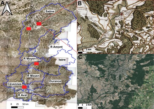
The work was made possible by the combination of two processes, topographic rendering and triangulation work. The topographic rendering was used by army cartographers (Pelletier, 1990). After the triangulation work, the filling of the Cassini map began in 1747, at a scale of 1/86 400. The map was designed to present a comprehensive view of the land use of the French territory, and the time of its making represented the peak of the climatic crisis of the LIA and the strongest historical human imprints on the Alpine and Piedmont landscapes.

For a definition of the present conditions to compare with those recorded in the Cassini map, we use the Corine Land Cover (CLC) inventory, resulting from a European program established by the European Environment Agency. With the first version completed in 1990 and the latest revision in 2018, it assigns a land cover type over the entire surface of 38 European states at a scale of 1:100 000. The CLC maps surfaces of a minimum size of 25 hectares, and the whole map is associated with an occupation mode. The land-use types are obtained by photo-interpretation of satellite images with a precision of 10 meters for the 2018 edition.

3.2. Methods

3.2.1. Semantic segmentation

The semantic segmentation of the Cassini maps was aimed at extracting feature elements such as land use classes. The task consisted of generating classification maps where each pixel is assigned to a value indicating either a feature class or the image background. The small variations in image texture make this task complex, and we therefore considered that a deep convolutional neural network approach could be valuable.

Our attention was turned toward encoder-decoder architectures, which have been demonstrated to be efficient for semantic segmentation tasks (Shelhamer et al., 2017). The encoder allows, through a succession of convolution operations and down-sampling layers, the extraction of features of growing levels of abstraction. The decoder then reconstitutes the segmented image through a succession of up-sampling layers followed by convolution operations. In the last layer, the reconstructed image has a pixel-to-pixel correspondence with the input image.

The U-Net++ architecture (Zhou et al., 2018) is an improved version of the original U-Net, which is a well-known encoder-decoder network architecture (Ronneberger et al., 2015). In both architectures, the spatial resolution lost during the contraction path is partially recovered through skip connections, allowing the concatenation of approximative and abstract feature maps of the encoder with accurate and low-level feature maps of the decoder. However, U-Net++ was proposed with a redesigning of the skip pathways to minimize the semantic gap between the encoder and decoder (Figure 2). In this configuration, the two paths are connected through a series of nested and dense skip pathways that fast-forward high-resolution feature maps from the encoder to the decoder.

Figure 2. Overview of the U-Net++ architecture for our specific output. The encoder and decoder sub-networks are connected through a series of nested dense convolutional blocks. The operations are as follows. Convolution (3 × 3) followed by batch normalization with a ReLU activation function allows extraction of feature elements. Max pooling (2 × 2) is used to down-sample the input image to reduce the number of parameters and capture fine-grained features. Transposed convolution is used to up-sample feature maps. Concatenation is used to combine feature maps from the two sub-networks. The first convolution applied to the input image contains 32 filters. The resulting number of channels (or features maps) is doubled after each convolution, whereas the feature maps are downsized by a factor of two after each max-pooling layer.

Representation of the architecture of the U-Net ++ network. On the left, an extract of the Cassini map. In the middle, the colored bricks representing the different phases. On the right, as an output, the result of the learning by the network.

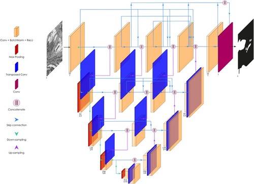
The decoder consists of a succession of transposed convolution operations (2 × 2) and concatenation followed by convolution, batch normalization, and ReLU activation functions. Skip connections in the original U-Net are replaced by dense convolution blocks (Huang et al., 2017). Finally, the output image is generated by concatenating low-level dense-block output layers and passing them through a convolution layer, as proposed by Peng et al. (2019), Peng et al. (2019) and Xu et al. (2020).

The training dataset contained 30 images with a size of 4 481 253 pixels. Because of the limited number of images, patch-based training was conducted using a set of 16 384 pixels with half-overlapping patches (Hammoumi et al., 2021). During the inference, a stochastic distribution process was performed on the patches to overcome artifacts at the edges (Hammoumi et al., 2021). For 20 epochs, the network was monitored using a binary cross-entropy loss function and an Adam optimizer (Diederik & Ba, 2015) with a learning rate of 3e⁻⁴.

The architecture of the U-Net++ network was adapted to provide accurate results with a small set of images. For each class, a dataset of 30 images of the same size underwent half overlapping patch learning (Hammoumi et al., 2021). The 30 images of each class were binary contours; e.g. for forests, each forest area on the image was submitted as a white filter and areas outside of the forests as a black filter. To prepare the data for the learning base, 6 h of manual segmentation were required to create the learning base for each class (forest, heath and arboriculture), and 10 h were required for the hydrology. The area covered by these class segmentations represented 10% of the total area (100 000 km²); thus, the time saving compared with a full manual segmentation was considerable.

3.2.2. Comparison

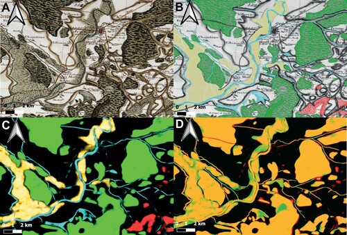
Several classes were defined to quantify the state of land use at the end of the eighteenth century. We segmented the Cassini map into four main classes: forest, heath, arboriculture, and hydrography features (Figure 3). These classes are in turn composed of several more precise types of vegetation: forest includes figures of trees, wood, pines, and fir trees; heath includes moors, scrub, and marshes; and arboriculture includes olive trees and vineyards. The selected classes were defined based on their importance with respect to soil erosion, for use in future studies throughout the basin.

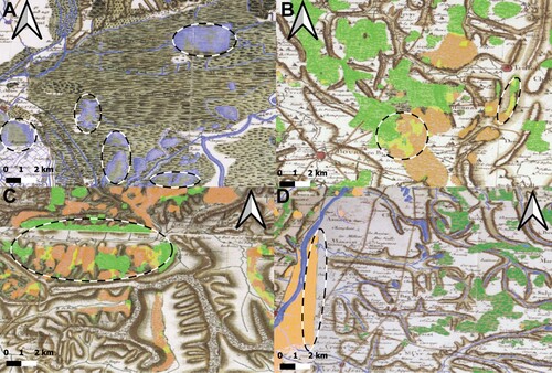
Figure 3. A: The area of Auxonne, B: Manual segmentation of the different classes, C: Results of the semantic segmentation, D: Comparison between the two segmentations, yellow = same detection, red = additional semantic detection, green = missing semantic detection.

Series of 4 images representing all Auxonne and its surroundings A: Cassini map. B: Cassini map in background and over it semi-transparent green, yellow, blue or red polygons, each representing a mode of occupation. C: Result of learning, black background, over it, green, yellow, blue or red polygons, each representing a mode of occupation. D: Result of the superposition between B and C. Black background. Over it, orange, green or red polygons, depending on the correspondence or not.

To enable spatial comparisons of soil distribution, seven sub-regions (Figure 1) were distinguished on the basis of their hydrographic limits: Saône, Durance, Isère, Cévennes, Upstream Rhône, Middle Rhône valley, and Downstream Rhône. These sub-regions are characterized by different morphostructural, bioclimatic, and hydroclimatic conditions (Bravard & Provansal, 2008; Parrot, 2015). According to the climatic and anthropic conditions present at the time of the realization of the Cassini map, we expect to observe less extensive surface coverage by forests, heaths, and arboriculture in comparison with recent times. Inversely, the hydrological network should be more extensive than it currently is.

4. Results

Segmentation tests were performed on four different areas (Figure 1), and the results of these segmentations are summarized in Table 1. We present the percentage correspondence between the automatic and manual segmentation for each class (Table 1(A)). To test the accuracy of the results obtained on this set of four images, the intersection-over-union (IOU) index was used to calculate the overlap rate between the manual and automatic segmentations.

Table 1. A: The results for the four illustrated areas. B: Comparisons of the Cassini results with previous published quantitative analyses (Guo et al., 2018; Herrault et al., 2015; Petitpierre, 2021).

A		Forest	Heaths	Arboriculture	Hydrology
Test area 1	Presence	95.6%	89.1%	91.1%
	Absence	95.9%	98.1%	99.2%
	IOU	95.8%	96.7%	98.7%
Test area 2	Presence	92.1%			91.3%
	Absence	97.6%			96.0%
	IOU	96.7%			95.7%
Test area 3	Presence	96.5%	89.4%	93.6%	80.9%
	Absence	97.9%	98.7%	99.4%	97.8%
	IOU	97.5%	97.6%	99.3%	96.7%
Test area 4	Presence		86.2%	89.4%	80.4%
	Absence		93.5%	97.4%	97.9%
	IOU		92.2%	95.8%	97.1%
Mean	Presence	94.7%	88.2%	91.4%	84.2%
	Absence	97.1%	96.8%	98.7%	97.2%
	IOU	96.7%	95.5%	98.0%	96.6%
B		Urban maps	Old map of Paris	Forest of Etat-Major	Our Study
Precision		99.4%	92.9%	93.4%	89.6%
Confidence index		93.6%	89.1%	91.0%	96.7%

The results for the four illustrated area. The accuracy of the segmentation is calculated for each occupancy mode according to 3 factors, the good detection of the presence of the class, the absence of the class and the confidence index. An average of the 4 test areas is proposed for each occupancy mode. B: Comparisons of the accuracy and confidence index of our study and previous study (Guo et al., 2018 ; Herrault et al., 2015 ; Petitpierre, 2021).

The best-segmented class was the forest class (94.7%), followed by the arboriculture (91.4%), heath (88.2%), and hydrology classes (84.2%). The lower precision for the hydrology class can be explained by the manual segmentation of the hydrographic features, which was more complicated than that of the other classes because it involved segmentation of lines irregularly varying in width, rather than zones. A visual comparison between the automated segmentation and manual segmentation of the hydrographic class on the Cassini map shows the good resolution achieved for this class (Figure 3). The IOU indices were 96.6% for the forest class, 95.5% for the heath class, 98.2% for the tree class, and 96.5% for the hydrology class. The above results attest to the quality of the automated segmentation of the different classes (Table 1(A)).

A large-scale segmentation was then performed on the different sub-basins, and we present the results for each sub-basin in Figure 4. Major differences were observed between the Cassini map and the CLC map. The four selected land use classes cover 28.1% of the total area of the Cassini map compared with 49.4% on the CLC.

Figure 4. Comparison of Cassini map and 2018 Corine Land Cover map occupancy classes according to individual sub-basins and the overall watershed.

Four graphs, one for each mode of occupation, heaths, Arboriculture, Forest and Hydrology. On the ordinate axis, the surface covered in percentage, for the abscissa axis, the different sub-basins. In addition, the blue results for the map.

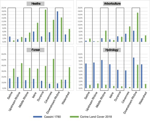
The forests on the CLC are 2.5 times more extensive than those on the Cassini map, with a maximum difference in the Cévennes sub-basin, where the forest currently covers 6.6 times the area covered at the end of the eighteenth century. The heathland and arboriculture classes currently cover 1.7 and 1.8 times more space at the basin scale, respectively, than when the Cassini map was made. Heaths show a maximum expansion in the Durance sub-basin, with a surface increase of 5.9 times the initial surface. The expansion in the area of the arboriculture class is substantial in the middle Rhone and downstream Rhone sub-basins, with increases of 3 and 2.6 times compared with the initial area. The results for the hydrographic class show a sharp contrast, with this class covering 7% of the basin at the time of the Cassini map, as opposed to 1.2% in the present day, with the surface area being up to 10 times greater on the Cassini maps. In the sub-basin of the Durance and the downstream Rhône, the area is only 1.3 times greater on the Cassini map than on the CLC, because the wide braided river beds that are well developed today were already present then.

5. Discussion

Our results can be compared with those presented in previous papers (Table 1(B)). In the semantic segmentation of a recent urban map, Guo et al. obtained an accuracy of 99.4% with a confidence index of 93.6% (Guo et al., 2018). In a study on other ancient maps, such as those of the city of Paris, Petitpierre (2021) found an accuracy of 92.9% and a confidence index of 89.1%, values that are close to those obtained in this study. In the case of forests, the work of Herrault et al. (2015) is very close to ours. On state maps made between 1818 and 1866, their study showed an average accuracy of 93.4%, very close to the value of 94.7% in this study.

The semantic segmentation applied in this study allows quantitative data for several land use classes to be rapidly extracted from a historical map for regions outside of forests (Vallauri et al., 2012) and cities/communication networks (Motte & Vouloir, 2007). The accuracy obtained by this segmentation is encouraging, because the results were obtained on raw data without preprocessing. It seems unnecessary to push the accuracy of the segmentation towards 100% because the data on the map are representative, not exhaustive (e.g. in Figure 5, the absence of small woodlands and copses sometimes blurs boundaries and differences between parts of the map). The variable accuracy for the different classes can be partly explained by the quality of the manual segmentation, particularly for the hydrographic class. In addition, some elements of the map can cause problems (Figure 4), with textual inscriptions and topographic lines impacting the quality of the segmentation. Another factor to consider is that not all parts of the map were drafted at the same time or by the same cartographers, and it is therefore possible that some of the map’s junctions are inconsistent (Figure 5). The results could possibly be improved by filtering the raw images to remove these features.

Figure 5. Presentation of the types of errors in the segmentation. A: Poor detection of the hydrographic class for some lake/ponds. B/C: Topography lines on heathland features distort the segmentation leading to a false classification as forest. D: A bad transition between two maps with disappearance of heathland features in the left part of the map.

Set of 4 different extracts from the Cassini map, each in the background. A: In blue, the representation of the hydrological surfaces, visible defects are circled. In particular for the filling of ponds. B: Forests in green and heaths in orange overlap in some places on the map, these areas are circled. C: Forests in green and heaths in orange, the extract presents a join in two pieces of map which are not coherent between them, there is a cut in the continuity of the ground occupation, this zone is surrounded. D: Again, the joint between two pieces of card. The hydrological network, in blue, is coherent, but the heaths, in orange, are not.

The segmentation of the Cassini map (Main Map) provides a quantitative estimate of the landscape pattern of the Rhone basin during the LIA climatic deterioration, at a time when aerial photography and satellite imagery did not exist. This work was carried out within the framework of a geomorphological study of the Rhone delta that requires an understanding of the recent evolution of the Rhone basin. Our results provide the first quantification of the erosive potential of the Rhône basin at the end of the eighteenth century. When combined, the identified classes cover only 28.1% of the total basin surface, with 65% of the Cassini map presenting areas with no figures. This part seems to correspond mainly to pasture and arable land, both being important in regard to areal erosion.

These results required quick input of data with limited time resources. The semantic segmentation allowed us to obtain, within a reasonable time, the land uses described in the Cassini map, with precision suitable for use in further analyses. Moreover, the results of the segmentation can be generated again using the freeware ‘Plug-Im!’ (https://www.plugim.fr/plugin/list), for which we provide a trained network and example images.

Our results show substantial differences between the Cassini map classes and the corresponding classes on the CLC 2018 map (Figure 6). As specified in the Results section, forests cover 2.5 times more surface today than they do in the Cassini map, with the largest differences occurring in the Cevennes and Durance sub-basins, both being mountainous regions associated with a present-day Mediterranean climate (Parrot, 2015). These differences between the Cassini map and the CLC can be explained by a cooler climate allowing the expansion of glaciers to the alpine valleys (Bradley & Jones, 1993), a slight decrease in the timberline in the high mountains because of the high use of wood for heating (Jandot, 2017), more intense pastoralism, and an increase in cultivated land in a period of demographic expansion. Another aspect or bias that needs to be discussed is that the Cassini map does not represent all wooded areas with a size of 5 hectares or less, and the wooded area obtained is, apparently, 20% less than the true forest area at that time (Vallauri et al., 2012), which would increase the proportion from 14.7% to 17.6%. Comparisons are therefore possible for a large-scale study such as ours, but the Cassini map may not be sufficiently accurate for a small-scale study. The observed decrease is logical given the low temperatures and high use of wood at that time, and the figures obtained in this study are comparable to those of Vallauri et al. (2012), who obtained an average forest surface of 12.6% for France as a whole and 17.6% for the regions of the Rhone basin through manual segmentation. For heaths, the present area of coverage is almost twice that on the Cassini map. This difference can be explained by human activities and climatic conditions that do not facilitate the development of this environment, and also by a possible under-representation during the realization of the Cassini map. This hypothesis could be verified by the contribution of the Napoleonic land survey map. The current area covered by arboriculture is currently twice as large as that on the Cassini map, which can be explained by vineyard expansion (Durbiano, 1988) and olive growing.

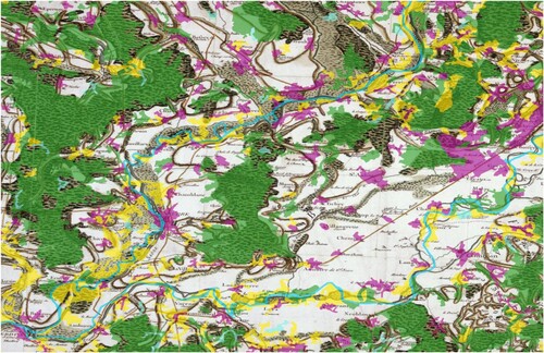
Figure 6. Overlay of the Auxonne area of the Cassini map presented in Figure 2 and the Corine Land Cover (CLC) data for the same area. The CLC data are shown with transparency: Green = Forest, Yellow = Heath, Purple = Urbanism, Blue = Hydrology.

Extract of the map of cassini on Auxonne and its surroundings in background. Over it, data from the Corine Land Cover program, Green = Forest, Yellow = Heath, Purple = Urbanism, Blue = Hydrology.

The area covered by hydrographic features in Cassini is 7% (Main Map), which is several times higher than the 1.2% on the CLC. This difference can be explained by two factors. The first is related to the figurative representation at the local scale (Dainville, 1955), and the hydrological network may have been overestimated; the differences in Figure 4 therefore need to be qualified. The second factor is the fluvial metamorphosis recorded at LIA, with many channel sections shifting from meandering to braided patterns due to an increase in flood frequency (Arnaud et al., 2012; Pichard et al., 2017) and sediment delivery (Bravard, 2010). The large areas occupied by hydrographic features illustrate the fluvial style required for strong sediment transport at this time (Arnaud-Fassetta & Provansal, 1999; Bravard et al., 1997 Maillet et al., 2006b). The importance of the differences observed in the Saône must therefore be qualified because this basin did not experience the hydrological modifications recorded after the end of the LIA, which are visible in the Durance or Isère. For the Saône it would therefore be the quality of representation of the map that would be the main factor. Post-LIA developments such as submersible dikes in 1840, low dikes in 1876, groins in 1880, Girardon traps in 1884, dams starting from 1948, and aggregate extraction, led to the incision of riverbeds, channelization of the main riverbed, and abandonment of secondary riverbeds (Bravard et al., 1999; Fruget & Dessaix, 2003; Parrot, 2015; Piégay et al., 2004; Poinsard & Salvador, 1993; Tena et al., 2020; Vázquez-Tarrío et al., 2019).

6. Conclusion

Semantic segmentation with a CNN allowed us to obtain an accuracy of up to 90% on a basin of nearly 100 000 km² represented by the Cassini map. This segmentation provided reliable results from a dataset of 30 images per class, which prevents a considerable time saving in comparison with manual segmentation. The time required was 10 times lower than that required for a fully manual segmentation. Moreover, the process was relatively easy to apply. At the end of the eighteenth century, forests covered between 14.7% and 17.6% of the total area of the Rhône basin, illustrating the low afforestation rate already identified in the literature. The segmentation resulted in an area of 4.3% for heathland, 2.1% for arboriculture, and 7% for hydrographic features. These results illustrate a period of climatic disturbance with very high human pressure on lands, favoring phases of high hydrological activity, denudation of the slopes due to the cooling period, and land use activity favoring sedimentary transport. These results are the first step in a study to reconstruct the erosion potential in the basin from the end of the eighteenth century (at the height of the LIA crisis) to the present day. The accuracy of the semantic segmentation is encouraging for the future, and it should be possible to quickly deploy it on other land occupation maps. The next objective will be to complete the Cassini map data (which only cover 28% of the total surface) with the Napoleonic land survey map and the Sardinian map to try to calculate an erosion balance using the RUSLE model.

Software

Map extraction was performed using Qgis 3.22 Biatowieza software. The manual contouring phases were performed using Adobe Illustrator. The algorithm used for network training was a script in python language written in the Jupyter notebook. Plug Im! software (https://www.plugim.fr/plugin/list) was used to visualize the results of the training.

Disclosure statement

No potential conflict of interest was reported by the author(s).

Data availability statement

The data that support the findings of this study are available from the corresponding author, Théo Martinez, upon reasonable request.

References

- Arnaud, F., Révillon, S., Debret, M., Revel, M., Chapron, E., Jacob, J., & Magny, M. (2012). Lake Bourget regional erosion patterns reconstruction reveals Holocene NW European Alps soil evolution and paleohydrology. Quaternary Science Reviews, 51, 81–92. https://doi.org/10.1016/j.quascirev.2012.07.025
- Arnaud-Fassetta, G., & Provansal, M. (1999). High-frequency variations of water flux and sediment discharge during the Little Ice Age (1586–1725 AD) in the Rhône Delta (Mediterranean France). Relationship to the catchment basin. In J. Garnier & J. M. Mouchel (Eds.), Man and River Systems. Developments in Hydrobiology (Vol. 146, pp. 241–250). Springer. https://doi.org/10.1007/978-94-017-2163-9_25
- Bradley, R. S., & Jones, P. D. (1993). Little ice age’ summer temperature variations: Their nature and relevance to recent global warming trends. The Holocene, 3(4), 367–376. https://doi.org/10.1177/095968369300300409
- Bravard, J. P. (2010). Discontinuities in braided patterns: The River Rhône from Geneva to the Camargue delta before river training. Geomorphology, 117(3-4), 219–233. https://doi.org/10.1016/j.geomorph.2009.01.020
- Bravard, J. P., Amoros, C., Pautou, G., Bornette, G., Bournaud, M., Creuzé des Châtelliers, M., & Tachet, H. (1997). River incision in south-east France: Morphological phenomena and ecological effects. Regulated Rivers: Research & Management: An International Journal Devoted to River Research and Management, 13(1), 75–90. https://doi.org/10.1002/(SICI)1099-1646(199701)13:13.0.CO;2-6
- Bravard, J. P., Landon, N., Peiry, J. L., & Piégay, H. (1999). Principles of engineering geomorphology for managing channel erosion and bedload transport, examples from French rivers. Geomorphology, 31(1-4), 291–311. https://doi.org/10.1016/S0169-555X(99)00091-4
- Bravard, J. P., & Provansal, M. (2008). Le Rhône en 100 Questions, ZABR, GRAIE, Villeurbanne, 295 p.
- Dainville, F. D. (1955). La carte de Cassini et son intérêt géographique. Bulletin de L'Association de géographes français, 32(251), 138–147. https://doi.org/10.3406/bagf.1955.8014
- Diederik, P. K., & Ba, J. (2015). Adam: A method for stochastic optimization. CoRR, abs/1412.6980.
- Dunesme, S., Piégay, H., & Mustière, S. (2022). Automatic vectorization of fluvial corridor features on historical maps to assess riverscape changes. Cartography and Geographic Information Science, 49(6), 512–527. https://doi.org/10.1080/15230406.2022.2091661
- Durbiano, C. (1988). L'expansion du vignoble des Côtes du Rhône méridionales. Méditerranée, 65(3), 3–11. https://doi.org/10.3406/medit.1988.2560
- Francou, B., & Vincent, C. (2007). Les glaciers à l’épreuve du climat. IRD Editions.
- Fruget, J. F., & Dessaix, J. (2003). Changements environnementaux, dérives biologiques et perspectives de restauration du Rhône français après 200 ans d’influences anthropiques. VertigO-la Revue électronique en Sciences de L'environnement, 4(3). https://doi.org/10.4000/vertigo.3832
- Fuchs, R., Verburg, P. H., Clevers, J. G., & Herold, M. (2015). The potential of old maps and encyclopaedias for reconstructing historic European land cover/use change. Applied Geography, 59, 43–55. https://doi.org/10.1016/j.apgeog.2015.02.013
- García, J. H., Dunesme, S., & Piégay, H. (2020). Can we characterize river corridor evolution at a continental scale from historical topographic maps? A first assessment from the comparison of four countries. River Research and Applications, 36(6), 934–946. https://doi.org/10.1002/rra.3582
- Guo, Z., Shengoku, H., Wu, G., Chen, Q., Yuan, W., Shi, X., Shao, X., Xu, Y., & Shibasaki, R. (2018). Semantic segmentation for urban planning maps based on U-Net. IEEE International Symposium on Geoscience and Remote Sensing, 6187–6190. https://doi.org/10.1109/IGARSS.2018.8519049
- Hammoumi, A., Moreaud, M., Ducottet, C., & Desroziers, S. (2021). Adding geodesic information and stochastic patch-wise image prediction for small dataset learning. Neurocomputing, 456, 481–491. https://doi.org/10.1016/j.neucom.2021.01.108
- Herrault, P. A., Sheeren, D., Fauvel, M., & Paegelow, M. (2015). Vectorisation automatique des forêts dans les minutes de la carte d’état-major du 19e siècle. Revue Internationale de Géomatique, 25(1), 35–51. https://doi.org/10.3166/RIG.25.35-51
- Huang, G., Liu, Z., Van Der Maaten, L., & Weinberger, K. (2017). Densely connected convolutional networks. IEEE conference on computer vision and pattern recognition (CVPR), Honolulu, HI, USA, pp. 2261–2269. https://doi.org/10.1109/CVPR.2017.243.
- Jandot, O. (2017). Les délices du feu: L'homme, le chaud et le froid à l'époque moderne. Editions Champ Vallon.
- Koerner, W., Cinotti, B., Jussy, J. H., & Benoît, M. (2000). Evolution des surfaces boisées en France depuis le début du XIXème siècle: identification et localisation des boisements des territoires agricoles abandonnés. Revue forestière française, 52(3), 249–269. https://doi.org/10.4267/2042/5359
- Maillet, G. M., Sabatier, F., Rousseau, D., Provansal, M., & Fleury, T. J. (2006a). Connexions entre le Rhône et son delta (partie 1) : évolution du trait de côte du delta du Rhône depuis le milieu du XIXe siècle. Geomorphologie, 12(2), 111–124. https://doi.org/10.4000/geomorphologie.558
- Maillet, G. M., Vella, C., Provansal, M., & Sabatier, F. (2006b). Connexions entre le Rhône et son delta (partie 2): Évolution du trait de côte du delta du Rhône depuis le début du XVIIIe siècle. Geomorphologie, 12(2), 125–140. https://doi.org/10.4000/geomorphologie.559
- Motte, C., & Vouloir, M. C. (2007). Le Site cassini. ehess. fr: Un Instrument d’Observation pour une Analyse du Peuplement. Bulletin du Comité Français de Cartographie, 191, 68–84. http://geoprodig.cnrs.fr/items/show/189128
- Notebaert, B., Berger, J. F., & Brochier, J. L. (2014). Characterization and quantification of Holocene colluvial and alluvial sediments in the Valdaine Region (southern France). The Holocene, 24(10), 1320–1335. https://doi.org/10.1177/0959683614540946
- Notebaert, B., & Piégay, H. (2013). Multi-scale factors controlling the pattern of floodplain width at a network scale: The case of the Rhône basin, France. Geomorphology, 200, 155–171. https://doi.org/10.1016/j.geomorph.2013.03.014
- Olivier, J. M., Carrel, G., Lamouroux, N., Dole-Olivier, M. J., Malard, F., Bravard, J. P., & Barthélemy, C. (2022). The Rhône river basin. In Rivers of Europe (pp. 391–451). Elsevier.
- Parrot, E. (2015). Analyse spatio-temporelle de la morphologie du chenal du Rhône du Léman à la Méditerranée (Doctoral dissertation, Lyon 3).
- Pelletier, M. (1990). La Carte de Cassini: L’extraordinaire aventure de la carte de France. Presses Ponts et Chaussées.
- Peng, C., Li, Y., Jiao, L., Chen, Y., & Shang, R. (2019). Densely based multi-scale and multi-modal fully convolutional networks for high-resolution remote-sensing image semantic segmentation. IEEE Journal of Selected Topics in Applied Earth Observations and Remote Sensing, 12(8), 2612–2626. https://doi.org/10.1109/JSTARS.2019.2906387
- Peng, D., Zhang, Y., & Guan, H. (2019). End-to-end change detection for high resolution satellite images using improved UNet++. Remote Sensing, 11(11), 1382. https://doi.org/10.3390/rs11111382
- Petitpierre, R. (2021). Neural networks for semantic segmentation of historical city maps: Cross-cultural performance and the impact of figurative diversity. arXiv preprint arXiv:2101.12478.
- Pichard, G., Arnaud-Fassetta, G., Moron, V., & Roucaute, E. (2017). Hydro-climatology of the Lower Rhône Valley: historical flood reconstruction (AD 1300–2000) based on documentary and instrumental sources. Hydrological Sciences Journal, 62(11), 1772–1795. https://doi.org/10.1080/02626667.2017.1349314
- Piégay, H., Walling, D. E., Landon, N., He, Q., Liébault, F., & Petiot, R. (2004). Contemporary changes in sediment yield in an alpine mountain basin due to afforestation (the upper Drôme in France). Catena, 55(2), 183–212. https://doi.org/10.1016/S0341-8162(03)00118-8
- Poinsard, D., & Salvador, P. G. (1993). Histoire de l’endiguement du Rhône à l’aval de Lyon. In Actes du colloque international Le fleuve et ses métamorphoses, Lyon, 13–15 mai 1992, pp. 299–314.
- Prosper-Laget, V., Pichard, G., Miramont, C., & Sivan, O. (2009). Les conditions climatiques de la torrentialité au cours du Petit Age Glaciaire en Provence. Archéologie du Midi Médiéval, 27(1), 157–167. https://doi.org/10.3406/amime.2009.1894
- Ronneberger, O., Fischer, P., & Brox, T. (2015). U-Net: Convolutional networks for biomedical image segmentation. In: Navab N., Hornegger J., Wells W., Frangi A. (Eds.), Medical image computing and computer-assisted intervention – MICCAI 2015. MICCAI 2015. Lecture notes in computer science, vol. 9351. Springer. https://doi.org/10.1007/978-3-319-24574-4_28.
- Rousseau, L. (1960). De l’influence du type d’humus sur le développement des plantules de sapins dans les Vosges. In Annales de l'école nationale des eaux et forêts et de la station de recherches et expériences. ENEF, Ecole nationale des eaux et forêts, Nancy (FRA).
- Salvador, P.-G., & Berger, J.-F. (2014). The evolution of the Rhone river in the Basses Terres basin during the Holocene (Alpine Foothills, France). Geomorphology, 204, 71–85. https://doi.org/10.1016/j.geomorph.2013.07.030
- Sclafert, T. (1959). Cultures en Haute-Provence: Déboisements et pâturages au Moyen Âge (Vol. 4). Editions De l'Ecole des hautes etudes en sciences sociales.
- Shelhamer, E., Long, J., & Darrell, T. (2017). Fully convolutional networks for semantic segmentation. IEEE Transactions on Pattern Analysis and Machine Intelligence, 39(4), 640–651. https://doi.org/10.1109/TPAMI.2016.2572683
- Surell, A. (1847). Mémoire sur l’amélioration des embouchures du Rhône. Impr. Ballivet et Fabre.
- Tasar, O., Tarabalka, Y., & Alliez, P. (2019). Incremental learning for semantic segmentation of large-scale remote sensing data. IEEE Journal of Selected Topics in Applied Earth Observations and Remote Sensing, 12(9), 3524–3537. https://doi.org/10.1109/JSTARS.2019.2925416
- Tena, A., Piégay, H., Seignemartin, G., Barra, A., Berger, J. F., Mourier, B., & Winiarski, T. (2020). Cumulative effects of channel correction and regulation on floodplain terrestrialisation patterns and connectivity. Geomorphology, 354, 107034. https://doi.org/10.1016/j.geomorph.2020.107034
- Vallauri, D., Grel, A., Granier, E., & Dupouey, J. L. (2012). Les forêts de Cassini. Analyse quantitative et comparaison avec les forêts actuelles (Doctoral dissertation, WWF).
- Vázquez-Tarrío, D., Tal, M., Camenen, B., & Piégay, H. (2019). Effects of continuous embankments and successive run-of-the-river dams on bedload transport capacities along the Rhône River, France. Science of The Total Environment, 658, 1375–1389. https://doi.org/10.1016/j.scitotenv.2018.12.109
- Xu, W., Deng, X., Guo, S., Chen, J., Sun, L., Zheng, X., Xiong, Y., Shen, Y., & Wang, X. (2020). High-resolution u-net: Preserving image details for cultivated land extraction. Sensors, 20(15), 4064. https://doi.org/10.3390/s20154064
- Zhou, Z., Rahman Siddiquee, M. M., Tajbakhsh, N., & Liang, J. (2018). Unet++: A nested U-Net architecture for medical image segmentation. In: Stoyanov D. (Eds.), Deep learning in medical image analysis and multimodal learning for clinical decision support. DLMIA 2018, ML-CDS 2018. Lecture notes in computer science, vol. 11045. Springer. https://doi.org/10.1007/978-3-030-00889-5_1.