Glacial geomorphology of the Republic of Karelia, northwest Russia: the Younger Dryas-early Holocene ice marginal zone

ABSTRACT

At present, there remains uncertainty surrounding the Younger Dryas-early Holocene glacial history of the Fennoscandian Ice Sheet in northwest Arctic Russia. This stems from a lack of high-resolution ice sheet-scale geomorphological data in the region. To address this, this paper presents 15,355 meltwater and morainic landforms in a new large-scale, glacial geomorphological map of the Younger Dryas-early Holocene ice marginal zone in the Republic of Karelia, northwest Russia. Individual landforms were mapped from relief-shaded renditions of the 2 m resolution ArcticDEM alongside 1 m resolution Esri World Imagery data in a Geographic Information System (GIS). The map, which is presented at a scale of 1: 675,000, will form the basis of a palaeo-glaciological reconstruction of northwest Russia that will inform on ice sheet dynamics – at both a regional- and ice sheet-scale – and provide an important framework through which numerical ice sheet models can be constrained.

KEYWORDS:

• Glacial geomorphology
• Fennoscandian Ice Sheet
• Republic of Karelia
• Russia
• Finland
• Younger Dryas

1. Introduction

The Younger Dryas (c. 12.8–11.7 ka) is a key stadial for palaeo-glaciologists and numerical ice sheet modellers investigating ice sheet dynamic responses to rapid climate change (Åkesson et al., 2018; Golledge et al., 2008, 2009; Hubbard, 1999; Patton et al., 2017; Rainsley et al., 2018). Thus, the Fennoscandian Ice Sheet (FIS) Younger Dryas ice marginal zone and ice sheet dynamics are largely well reconstructed from Quaternary geological data (Andersen et al., 1995; Hughes et al., 2016; Rainio et al., 1995; Stroeven et al., 2016). However, recent research on the Kola Peninsula and Russian Lapland, northwest Russia, demonstrates that existing ice sheet reconstructions that use small-scale Quaternary geological data cannot be relied upon (Boyes, Linch, et al., 2021; Hughes et al., 2016). Where large-scale glacial geomorphological mapping is employed (e.g. Boyes, Pearce, et al., 2021; Clark et al., 2018), a more robust palaeo-glaciological reconstruction is produced (e.g. Boyes et al., 2023a, 2023b; Clark et al., 2012, 2022). Previous reconstructions in the neighbouring Republic of Karelia, northwest Russia (Figure 1), also typically employ small-scale, field mapped Quaternary geological data that are limited to major end moraines, spreads of hummocky moraine, and glaciofluvial complexes (Biske, 1959; Ekman & Iljin, 1991; Niemelä et al., 1993; Petrov et al., 2014). Regional data on, for example, meltwater channels are lacking.

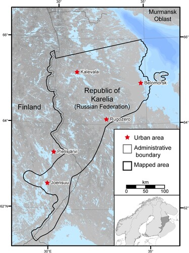
Figure 1. The Republic of Karelia, northwest Russia. The study area focusses on the Republic of Karelia with additional mapping in neighbouring Finland that captures complete landform assemblages. Topographic and bathymetric data in this figure are from the European Space Agency (2021), GEBCO Compilation Group (2023) GEBCO 2023 Grid. Topography is shaded grey with darker shades representing higher ground and bathymetry is shaded blue with darker shades representing greater depth. Lake data are from the Esri World Water Bodies dataset. Inset: The Fennoscandian Peninsula shaded and mapped area shaded light and dark grey respectively.

Study area map, showing the mapped area, regional borders, and major urban locations.

Recent advances in acquisition and availability of high-resolution remotely sensed imagery warrant a fresh investigation into formerly glaciated landscapes, such as northwest Russia. In this study, we extend large-scale glacial geomorphological mapping of northwest Arctic Russia (Boyes, Pearce, et al., 2021) into the Republic of Karelia. The Main Map focusses on meltwater and morainic landforms, thus providing the empirical data that are required for reconstructing ice marginal zones and retreat patterns. Subglacial bedforms are not mapped in this study because these landforms are not strictly required for reconstructing ice margin retreat patterns (Clark et al., 2012; Kleman & Borgström, 1996). The Republic of Karelia is a lowland landscape (∼0–400 m asl) bordered by Finland to the west and the White Sea to the east (Figure 1). The region's geology is dominated by Archean amphibolite and gneiss. This map will form the basis for future a palaeo-glaciological reconstruction focused on verifying previous Younger Dryas ice marginal zone reconstructions in northwest Russia.

2. Methods

To ensure that the glacial geomorphological datasets are consistent and can therefore be used alongside each other in a new reconstruction of ice sheet dynamics in northwest Russia, the methods used in the production of this glacial geomorphological map follow Boyes, Pearce, et al. (2021), which are based on Smith and Clark (2005), Greenwood and Clark (2008), Hughes et al. (2010), and Chandler et al. (2018), among others. The Main Map covers >69,000 km² of northwest Russia and represents over 155 hours of work.

2.1. Datasets and data processing

The Main Map is produced at a scale of 1: 675,000 based on two forms of high-resolution remotely sensed imagery: (i) the ArcticDEM Digital Surface Model (DSM), and (ii) Esri World Imagery. The ArcticDEM, which has a spatial resolution of 2 m (vertical accuracy of 2 m and horizontal accuracy of 3.8 m), was converted into hillshaded relief images for meaningful graphical and analytical purposes. To avoid azimuth bias, two hillshaded relief images were generated for the entire region with the sun placed at orthogonal angles of 45° (NE) and 315° (NW), generated with an illumination angle of 30°, and vertically exaggerated by three times to enhance subtle features (Figure 2). ‘Overhead’ and ‘multidirectional’ hillshade relief images (Boyes, Pearce, et al., 2021) were not produced because the low relief terrain across the study area renders these datasets unsuitable for identifying geomorphological features.

Figure 2. Examples of the imagery used during the digital mapping stage from the Republic of Karelia showing the resolution of data sources as well as different images derived from each data source. Two hillshaded relief images are derived from the 2 m resolution ArcticDEM: (a) azimuth 315°, illumination angle 30°; and (b) azimuth 45°, illumination angle 30°. Hillshaded relief images are vertically exaggerated three times to enhance subtle landforms. (c) Esri World Imagery data with up to 1 m spatial resolution is also displayed in full colour.

Examples of imagery used – hillshaded digital elevation models and satellite imagery.

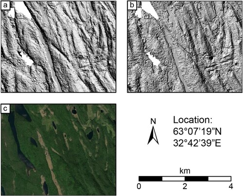
Esri World Imagery are orthorectified, georeferenced low- and high-resolution (spatial resolution of 1 m or better) satellite and aerial imagery of the Earth. The imagery is viewed in full-colour composite (Figure 2). Esri World Imagery was chosen over PlanetScope Ortho Scene data used by Boyes, Pearce, et al. (2021) because Esri World Imagery is freely available and ready to use for the entire study area, unlike PlanetScope Ortho Scene data, which requires a time-consuming process of data acquisition and processing. Nevertheless, the resolution of the Esri World Imagery is comparable to the PlanetScope Ortho Scene data and does not, therefore, negatively impact the ability to identify glacial geomorphology.

2.2. Mapping procedure

Google Earth Pro was used for 3D landform visualisation and virtual reconnaissance prior to digital mapping. Digital mapping was achieved through visual identification and onscreen vectorisation of individual landforms (discussed in Section 3) within a Geographic Information System (GIS) environment (Esri ArcMap^TM 10.8.1). Visual identification of glacial landforms was an integrated process involving several consultations of the DEM and satellite imagery. Repeated passes of the mapped area were made at a range of scales to ensure that features of all sizes were discernible on the imagery. Polylines map the crest-line of individual landforms while polygons map the break-of-slope outline of individual landforms. Individual vectors were smoothed for cartographic purposes, using a maximum allowable offset of 1 m to ensure the morphologies of the mapped landforms are not lost.

Landform identification, classification, and mapping style (i.e. polyline or polygon) follows the diagnostic criteria outlined by Boyes, Pearce, et al. (2021), and no new landform types were identified in this study. The different classifications of landforms identified in this study are discussed in section 3. Unlike Boyes, Pearce, et al. (2021), this study does not include subglacial bedforms because these landforms are not strictly required for reconstructing ice sheet margin positions (Clark et al., 2012; Kleman & Borgström, 1996); i.e. only meltwater and morainic landforms are mapped. Where more than one landform classification could be applied to a feature, the primary function of the feature is applied. For example, a meltwater channel could have subglacial and proglacial characteristics, but a subglacial classification is applied as the feature would have been this first.

Individual landforms also are attributed a subjective level of confidence weighted against the landform diagnostic criteria outlined so that future glacial reconstructions are developed with the greatest certainty by excluding lower confidence landforms. The confidence levels (the numbers refer to the value assigned in the attribute table) follow the criteria outlined by Boyes, Pearce, et al. (2021):

•  Low confidence (1): landform may not be of glacial origin, landform may be misinterpreted, and the boundaries of the mapped landform are likely inaccurate.

•  Medium confidence (2): landform is likely of glacial origin, landform may be misinterpreted, and the boundaries of the mapped landform may be inaccurate.

•  High confidence (3): landform is definitely of glacial origin, landform is correctly interpreted, and the boundaries of the mapped landform are accurate.

Elevation and bathymetric data for the base map are derived from the European Space Agency (2021) and the GEBCO Compilation Group (2023); these elevation data are for illustration purposes only and were not used during the digital mapping stage. The landform and basemap data are projected to the Geographic Coordinate System WGS1984 UTM Zone 36N. The map was exported from Esri ArcMap^TM 10.8.1 to Adobe Illustrator v26.5 for final production before being exported in PDF format.

3. Mapped glacial landforms

The Main Map includes a total of 15,355 glacial landforms mapped during this study, significantly extending the volume and detail of geomorphological data in the region. Notably, the Main Map contains the first assessment of meltwater channels in the Republic of Karelia. To avoid reconstruction bias that can be imposed by geopolitical borders, the mapping extends at least 5 km into neighbouring Finland and whole landforms are mapped rather than clipped to a border. Additionally, in places where apparent ice marginal zones significantly extend into Finland, the mapping is continued to the maximum extent of individual ice marginal zones with a ∼15 km buffer imposed. This approach will allow future reconstructions to consider unabridged landform assemblages rather than be constrained by artificial boundaries. Additionally, to allow the Main Map to be viewed alongside and overlapped with the map presented by Boyes, Pearce, et al. (2021), meltwater and morainic landforms mapped by Boyes, Pearce, et al. (2021) in the Republic of Karelia are also included: these data are not included in the supplementary information shapefiles nor are they discussed below.

To allow scrutiny of individual landforms the map is designed to be printed at A1 size (594 by 841 mm). For clarity, the Main Map does not distinguish individual landform classifications (e.g. lateral, subglacial, or proglacial meltwater channels) – these data can be viewed in the GIS shapefiles of the mapped landforms provided in the supplementary information. Moreover, the Main Map does not include the names of Younger Dryas ice marginal zones that are often applied by the scientific community – this is to ensure that a future glacial reconstruction is not influenced by pre-conceived ideas.

The landforms mapped in this study are discussed in this section and their occurrence and estimated completeness of mapped landforms can be presented in Table 1. The confidence rating and classification applied to each feature can be viewed in the attribute table of the shapefiles provided in the supplementary information. Although the purpose of the Main Map is for understanding the Younger Dryas-early Holocene glaciation it is likely that some mapped landforms are from different stages of the last glaciation. However, the relative age of the mapped glacial landforms will be explored in future studies.

Table 1. Mapped landforms, their occurrence, and estimated completeness (i.e. the percentage of glacial landforms thought to be mapped in this study).

Mapped landform	Mapping style	Occurrence By confidence level		Completeness (%)
Meltwater landforms
Meltwater channels	Polyline	Total:	4436	80
		High (3):	3383
		Medium (2):	1034
		Low (1):	19
Eskers	Polyline	Total:	3453	90
		High (3):	2558
		Medium (2):	669
		Low (1):	226
Glaciofluvial deposits	Polygon	Total:	1655	80
		High (3):	1429
		Medium (2):	213
		Low (1):	13
Morainic landforms
Moraine ridges	Polyline	Total:	1045	90
		High (3):	620
		Medium (2):	309
		Low (1):	116
Moraine deposits	Polygon	Total:	4766	90
		High (3):	2448
		Medium (2):	2117
		Low (1):	201
	Total number of mapped landforms		15,355

3.1. Meltwater landforms

Meltwater landforms include meltwater channels (relict channels that are the product of glacier ablation and meltwater flow; Greenwood et al., 2007), eskers (elongate, sinuous ridges composed of glaciofluvial sediments associated with subglacial drainage; Storrar et al., 2014), and glaciofluvial deposits (ice marginal accumulations of glaciofluvial material that mostly display planar surfaces; Bennett & Glasser, 2009; Hättestrand & Clark, 2006). Meltwater channels (Figure 3(a–c)) – with lengths ranging from ∼120 m to ∼25 km, with a median length of ∼1.1 km – are identified across the lowland landscape and, in some locations, superimposed on other glacial landforms. Following the criteria of Boyes, Pearce, et al. (2021), the meltwater channel types identified in the study area are:

•  Lateral: channels formed by meltwater flowing along ice margins; these features are typically observed on slopes oblique to contours.

•  Subglacial: channels formed by meltwater flowing beneath an ice sheet, typically orientated in the direction of ice flow with undulating long profiles.

•  Proglacial: channels formed by with meltwater flowing away from the ice sheet margins; these features are often adjacent to ice marginal landforms (e.g. moraine ridges) and indicate flow directly downslope.

  Figure 3. Examples of mapped meltwater landforms (red crestlines and outlines) expressed on hillshaded relief images of the ArcticDEM and Esri World Imagery.

  Examples of mapped landforms shown on hillshaded digital elevation models and satellite imagery.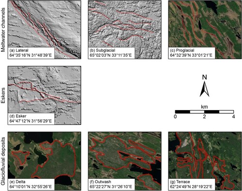

  

Eskers (Figure 3(d)), which are signatures of subglacial meltwater drainage (Greenwood et al., 2007; Storrar et al., 2014), range in length from ∼12 m to ∼16 km and display a median length of ∼740 m. Eskers are identified across the lowland landscape, often forming trails over 100 km long. Unlike other landforms mapped in this study, eskers are not sub-classified as this information is not strictly required for reconstructing former ice sheet dynamics (Kleman & Borgström, 1996).

Glaciofluvial deposits (Figure 3(e–g)) are predominantly identified alongside esker trails or probable ice marginal zones as large spreads up to 87 km². To support glacial interpretations, glaciofluvial deposits are classified based on the criteria of Boyes, Pearce, et al. (2021) as:

•  Delta: fan-shaped accumulations of glaciofluvial sediments.

•  Outwash: accumulations of glaciofluvial sediments that occur as large spreads (e.g. sandur).

•  Terrace: stepped accumulations of glaciofluvial sediments displaying planar upper surfaces and steep fluvial-erosional slopes.

Eskers (n = 3456) and subglacial meltwater channels (n = 4436) are the most prolific mapped landform across the study area. Eskers and subglacial meltwater channels reveal extensive subglacial drainage networks across the study area, indicating that the basal thermal regime of the FIS in this region was dominated by warm based conditions during deglaciation. Lateral meltwater channels are identified alongside other ice marginal landforms (e.g. glaciofluvial deposits and moraines), indicating that these features in the region outline ice margin positions rather than signifying cold-based glaciation. Glaciofluvial deposits, especially deltas, also signify ice margin positions in the study area and are often found in association with eskers, subglacial meltwater channels, and moraines.

3.2. Morainic landforms

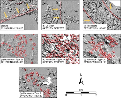
Morainic landforms (Figure 4) include moraine deposits (mounds, ridges, or spreads of glacigenic sediments; Bennett & Glasser, 2009) and moraine ridges (elongate ridge crests composed of glacigenic sediments; Bennett & Glasser, 2009). The spatial distribution of moraines is important to reconstructing ice margin positions. To allow additional interpretations of ice dynamics during ice sheet retreat and consistency across databases, moraines are classified following the criteria of Boyes, Pearce, et al. (2021) as:

•  End: ridges with defined crests that are aligned perpendicular to ice flow, demarcating the frontal margins of a glacier in a terrestrial environment.

•  De Geer: ridges aligned perpendicular to ice flow, demarcating the frontal margins of a grounded glacier in a sub-aqueous environment.

•  Interlobate: tabular ridges with steep slopes and hummocky or multi-crested upper surfaces, which form at the edge-to-edge contact of two ice margins.

•  Hummock – Type 2a: irregular morainic topography displaying complex ring, ridge, and hummock morphologies occurring in large spreads (up to 80 km²).

•  Hummock – Type 2b: irregular mounds and depressions, which can exist as large spreads (up to 100 km²).

•  Hummock – Type 2c: semi-ordered collections of tabular or ripple-like ridges transverse to ice flow direction.

•  Hummock – Type 3: irregular mounds that may be elongated and/or v-shaped, sometimes associated with subglacial drainage.

  Figure 4. Examples of mapped morainic landforms (red crestlines and outlines) expressed on hillshaded relief images of the ArcticDEM. Orange arrows point toward the ice contact slopes of moraines in the direction of inferred ice flow direction.

  

Moraines in the mapped area are typically arranged in prominent arcuate assemblages alongside glaciofluvial deposits. A prominent interlobate moraine complete with surficial eskers is also identified near Joensuu. These landforms assemblages indicate multiple palaeo-ice sheet margin positions in the Republic of Karelia.

4. Accuracy and completeness

The study area was mapped and examined for glacial landforms by two observers. However, to ensure consistency with regards to bias due to skill and experience in landform identification, all mapping was checked and validated by the lead author. The region was systematically examined, and mapping attempted to capture each individual landform. Moreover, ∼68% of the mapped landforms have been attributed the greatest confidence rating, high confidence (3) (Table 1). Thus, the map is regarded as an accurate reflection of the spatial distribution of glacial landforms. Post-glacial modification such as fluvial erosion and anthropogenic influence (the latter of which is minimal in this sparsely populated region) is apparent at the scale of individual landforms. Mapping, therefore, reflects the existing form of the landforms identified in the remotely sensed imagery.

It is estimated that the map is approximately 90% complete, i.e. we are confident that we have captured at least 90% of all meltwater and morainic landforms within the study area (Table 1). The remaining 10% of glacial landforms are likely to be concealed by lakes and reservoirs or obscured by the taiga forest that dominates the Republic of Karelia. However, the estimated completeness varies for some landform types (Table 1). For example, subtle spreads of glaciofluvial deposits are difficult to identify under dense tree cover, and possible meltwater channels can be confused with geological structures. Thus, more cautious completeness evaluations have been applied to glaciofluvial deposits and meltwater channels. Although not all landforms have been identified and included in this map, it is unlikely that this will have an adverse impact on a glacial reconstruction as these data are not crucial for the purposes of ice sheet-scale reconstructions (Clark et al., 2012; Kleman & Borgström, 1996).

The Main Map is a significant improvement on previous mapping attempts in the Republic of Karelia. For example, our esker dataset provides greater detail than the esker synthesis presented by Stroeven et al. (2016) (which is based on field mapping data presented by Niemelä et al., 1993) as it (i) maps individual esker segments rather than esker trails and (ii) identifies eskers in new locations, particularly in the north of the study area, where data are currently lacking. These developments are made possible by using high-resolution remotely sensed imagery including the ArcticDEM and Esri World Imagery, which allow entire landscapes to be rapidly mapped at large scales. Thus, the dataset associated with the Main Map supersedes previously published data on the region and will be the primary dataset for future palaeo-glaciological studies.

5. Conclusion

A total of 15,355 glacial landforms associated with the Younger Dryas-early Holocene glaciation of the Republic of Karelia in northwest Russia are mapped. This includes the first regional assessment of meltwater channels. The spatial distribution of mapped landforms reveals prominent arcuate landform assemblages and meltwater drainage networks characteristic of a lobate ice margin. The map presented here is a new large-scale regional assessment of glacial landforms in northwest Russia. This dataset provides crucial geomorphological data that will be used in a new glacial reconstruction of ice margin positions, retreat patterns, and ice sheet dynamics during the Younger Dryas-early Holocene transition. This reconstruction will provide an important framework through which numerical ice sheet models can be constrained and for targeting field investigations of palaeo-glaciation.

Software

Relief shaded visualisations of the ArcticDEM dataset, provided by the Polar Geospatial Center under NSF-OPP awards 1043681, 1559691, and 1542736 (Porter et al., 2018), were produced using Esri ArcMap^TM 10.8.1 (herein ArcMap). Satellite and aerial imagery were provided by Esri World Imagery. Google Earth Pro was used for 3D landform visualisation and virtual reconnaissance. On-screen digitisation of landform crest-line and break-of-slope was conducted in ArcMap. The map was produced in ArcMap and imported into Adobe Illustrator v26.5 where final layout work was completed prior to exporting as a PDF.

Acknowledgements

We particularly thank Lorna Linch and David Nash for discussions while producing the map. The British Society for Geomorphology are also thanked for funding support to present this map at their Annual Meeting. The Universities of Brighton and Sheffield are gratefully acknowledged for granting BMB Visiting Researcher status to complete this work. Bradley Goodfellow, Jasper Knight, Makram Murad-al-shaikh, Jiří Pánek, and Henry Patton are gratefully acknowledged for providing useful comments on both the map and manuscript.

Data availability statement

The data used in the production of this map are provided as supplementary material. These data are in the same format as Boyes, Pearce, et al. (2021) so that they can be directly compared and merged. The Esri shapefiles are projected using the GCS_WGS_1984 coordinate system (ESPG: 4326). The classifications and confidence ratings for each feature can be viewed in the attribute table of the shapefiles.

Disclosure statement

No potential conflict of interest was reported by the author(s).

Additional information

Funding

This work was undertaken while BMB was in receipt of a University of Brighton PhD Studentship. This publication is suppoted by the University of Sheffield Institutional Open Access Fund.

References

- Åkesson, H., Morlighem, M., Nisancioglu, K. H., Svendsen, J. I., & Mangerud, J. (2018). Atmosphere-driven ice sheet mass loss paced by topography: Insights from modelling the south-western Scandinavian Ice Sheet. Quaternary Science Reviews, 195, 32–47. https://doi.org/10.1016/j.quascirev.2018.07.004
- Andersen, B. G., Lundqvist, J., & Saarnisto, M. (1995). The Younger Dryas margin of the Scandinavian Ice Sheet — An introduction. Quaternary International, 28, 145–146. https://doi.org/10.1016/1040-6182(95)00043-I
- Bennett, M. R., & Glasser, N. F. (2009). Glacial geology: Ice sheets and landforms. John Wiley & Sons.
- Biske, G. S. (1959). Quaternary deposits and geomorphology of Karelia. Gosizdat Karelskoy ASSR.
- Boyes, B. M., Linch, L. D., Pearce, D. M., Kolka, V. V., & Nash, D. J. (2021). The Kola Peninsula and Russian Lapland: A review of late Weichselian glaciation. Quaternary Science Reviews, 267, 107087. https://doi.org/10.1016/j.quascirev.2021.107087
- Boyes, B. M., Linch, L. D., Pearce, D. M., & Nash, D. J. (2023a). The last Fennoscandian Ice Sheet glaciation on the Kola Peninsula and Russian Lapland (Part 1): Ice flow configuration. Quaternary Science Reviews, 300, 107871. https://doi.org/10.1016/j.quascirev.2022.107871
- Boyes, B. M., Linch, L. D., Pearce, D. M., & Nash, D. J. (2023b). The last Fennoscandian Ice Sheet glaciation on the Kola Peninsula and Russian Lapland (Part 2): Ice sheet margin positions, evolution, and dynamics. Quaternary Science Reviews, 300, 107872. https://doi.org/10.1016/j.quascirev.2022.107872
- Boyes, B. M., Pearce, D. M., & Linch, L. D. (2021). Glacial geomorphology of the Kola Peninsula and Russian Lapland. Journal of Maps, 17(2), 497–515. https://doi.org/10.1080/17445647.2021.1970036
- Chandler, B. M. P., Lovell, H., Boston, C. M., Lukas, S., Barr, I. D., Benediktsson, ÍÖ, Benn, D. I., Clark, C. D., Darvill, C. M., Evans, D. J. A., Ewertowski, M. W., Loibl, D., Margold, M., Otto, J. C., Roberts, D. H., Stokes, C. R., Storrar, R. D., & Stroeven, A. P. (2018). Glacial geomorphological mapping: A review of approaches and frameworks for best practice. Earth-Science Reviews, 185, 806–846. https://doi.org/10.1016/j.earscirev.2018.07.015
- Clark, C. D., Ely, J. C., Greenwood, S. L., Hughes, A. L. C., Meehan, R., Barr, I. D., Bateman, M. D., Bradwell, T., Doole, J., Evans, D. J. A., Jordan, C. J., Monteys, X., Pellicer, X. M., & Sheehy, M. (2018). BRITICE Glacial Map, version 2: A map and GIS database of glacial landforms of the last British-Irish Ice Sheet. Boreas, 47(1), 11–e8. https://doi.org/10.1111/bor.12273
- Clark, C. D., Ely, J. C., Hindmarsh, R. C. A., Bradley, S., Ignéczi, A., Fabel, D., Ó Cofaigh, C., Chiverrell, R. C., Scourse, J., Benetti, S., Bradwell, T., Evans, D. J. A., Roberts, D. H., Burke, M., Callard, S. L., Medialdea, A., Saher, M., Small, D., Smedley, R. K., … Wilson, P. (2022). Growth and retreat of the last British–Irish Ice Sheet, 31 000 to 15 000 years ago: The BRITICE-CHRONO reconstruction. Boreas, 51(4), 699–758. https://doi.org/10.1111/bor.12594
- Clark, C. D., Hughes, A. L. C., Greenwood, S. L., Jordan, C. J., & Sejrup, H. P. (2012). Pattern and timing of retreat of the last British-Irish Ice Sheet. Quaternary Science Reviews, 44, 112–146. https://doi.org/10.1016/j.quascirev.2010.07.019
- Ekman, I., & Iljin, V. (1991). Deglaciation, the Younger Dryas end moraines and their correlation in the Karelian A.S.S.R and adjacent areas. Geological Survey of Finland.
- European Space Agency, Sinergise. (2021). Copernicus global digital elevation model OpenTopography. Retrieved June 11, 2021, from https://doi.org/10.5069/G9028PQB.
- GEBCO Compilation Group. (2023). GEBCO 2023 grid. Retrieved May 15, 2023, from https://doi.org/10.5285/f98b053b-0cbc-6c23-e053-6c86abc0af7b.
- Golledge, N. R., Hubbard, A., & Sugden, D. E. (2008). High-resolution numerical simulation of Younger Dryas glaciation in Scotland. Quaternary Science Reviews, 27(9), 888–904. https://doi.org/10.1016/j.quascirev.2008.01.019
- Golledge, N. R., Hubbard, A. L., & Sugden, D. E. (2009). Mass balance, flow and subglacial processes of a modelled Younger Dryas ice cap in Scotland. Journal of Glaciology, 55(189), 32–42. https://doi.org/10.3189/002214309788608967
- Greenwood, S. L., & Clark, C. D. (2008). Subglacial bedforms of the Irish Ice Sheet. Journal of Maps, 4(1), 332–357. https://doi.org/10.4113/jom.2008.1030
- Greenwood, S. L., Clark, C. D., & Hughes, A. L. C. (2007). Formalising an inversion methodology for reconstructing ice-sheet retreat patterns from meltwater channels: Application to the British Ice Sheet. Journal of Quaternary Science, 22(6), 637–645. https://doi.org/10.1002/jqs.1083
- Hättestrand, C., & Clark, C. D. (2006). The glacial geomorphology of Kola Peninsula and adjacent areas in the Murmansk Region, Russia. Journal of Maps, 2(1), 30–42. https://doi.org/10.4113/jom.2006.41
- Hubbard, A. (1999). High-resolution modeling of the advance of the Younger Dryas ice sheet and its climate in Scotland. Quaternary Research, 52(1), 27–43. https://doi.org/10.1006/qres.1999.2055
- Hughes, A. L. C., Clark, C. D., & Jordan, C. J. (2010). Subglacial bedforms of the last British Ice Sheet. Journal of Maps, 6(1), 543–563. https://doi.org/10.4113/jom.2010.1111
- Hughes, A. L. C., Gyllencreutz, R., Lohne, O. S., Mangerud, J., & Svendsen, J. I. (2016). The last Eurasian ice sheets – A chronological database and time-slice reconstruction, DATED-1. Boreas, 45(1), 1–45. https://doi.org/10.1111/bor.12142
- Kleman, J., & Borgström, I. (1996). Reconstruction of palaeo-ice sheets: The use of geomorphological data. Earth Surface Processes and Landforms, 21(10), 893–909. https://doi.org/10.1002/(SICI)1096-9837(199610)21:10<893::AID-ESP620>3.0.CO;2-U
- Niemelä, J., Ekman, I., & Lukashov, A. (1993). Quaternary deposits of Finland and Northwestern part of Russian Federation and their resources: Map at 1: 1,000,000. Geological Survey of Finland and Institute of Geology, Karelian Science Centre of the Russian Academy of Sciences.
- Patton, H., Hubbard, A. L., Andreassen, K., Auriac, A., Whitehouse, P. L., Stroeven, A. P., Shackleton, C., Winsborrow, M., Heyman, J., & Hall, A. M. (2017). Deglaciation of the Eurasian ice sheet complex. Quaternary Science Reviews, 169, 148–172. https://doi.org/10.1016/j.quascirev.2017.05.019
- Petrov, O. V., Morozov, A. F., Chepkasova, T. V., Kiselev, E. A., Zastrozhnov, A. S., Verbitsky, V. R., Strelnikov, S. I., Tarnograd, V. D., Shkatova, V. K., Krutkina, O. N., Minina, E. A., Astakhov, V. I., Borisov, B. A., & Gusev, E. A. (2014). Map of quaternary formations of the territory of the Russian federation. Scale 1: 2 500 000. Ministry of Natural Resources and Ecology of the Russian Federation. (in Russian).
- Porter, C., Morin, P., Howat, I. M., Noh, M.-J., Bates, B., Peterman, K., Keesey, S., Schlenk, M., Gardiner, J., Tomko, K., Willis, M., Kelleher, C., Cloutier, M., Husby, E., Foga, S., Nakamura, H., Platson, M., Wethington, M., Williamson, C., … Bojesen, M. (2018). ArcticDEM version 3. Retrieved September 1, 2021, from https://doi.org/10.7910/DVN/OHHUKH
- Rainio, H., Saarnisto, M., & Ekman, I. (1995). Younger Dryas end moraines in Finland and NW Russia. Quaternary International, 28, 179–192. https://doi.org/10.1016/1040-6182(95)00051-J
- Rainsley, E., Menviel, L., Fogwill, C. J., Turney, C. S. M., Hughes, A. L. C., & Rood, D. H. (2018). Greenland ice mass loss during the Younger Dryas driven by Atlantic Meridional Overturning Circulation feedbacks. Scientific Reports, 8(1), 11307. https://doi.org/10.1038/s41598-018-29226-8
- Smith, M. J., & Clark, C. D. (2005). Methods for the visualization of digital elevation models for landform mapping. Earth Surface Processes and Landforms, 30(7), 885–900. https://doi.org/10.1002/esp.1210
- Storrar, R. D., Stokes, C. R., & Evans, D. J. A. (2014). Morphometry and pattern of a large sample (>20,000) of Canadian eskers and implications for subglacial drainage beneath ice sheets. Quaternary Science Reviews, 105, 1–25. https://doi.org/10.1016/j.quascirev.2014.09.013
- Stroeven, A. P., Hättestrand, C., Kleman, J., Heyman, J., Fabel, D., Fredin, O., Goodfellow, B. W., Harbor, J. M., Jansen, J. D., Olsen, L., Caffee, M. W., Fink, D., Lundqvist, J., Rosqvist, G. C., Strömberg, B., & Jansson, K. N. (2016). Deglaciation of Fennoscandia. Quaternary Science Reviews, 147, 91–121. https://doi.org/10.1016/j.quascirev.2015.09.016