Shoreline dynamics over last three decades and predictions for 2032 and 2042: a spatial analysis along the coastal stretch of Aruvi Aru and Kal Aru estuaries in Mannar district, Sri Lanka

ABSTRACT

The North-Western coastal stretch of the Aruvi Aru and Kal Aru estuaries in Sri Lanka's Mannar district faces increasing vulnerability due to coastal erosion, but comprehensive research has been lacking until now. This study aims to analyze shoreline changes from 1988 to 2022 and forecast future changes until 2042. Landsat satellite images and statistical parameters such as LRR and AoR were used to calculate erosion and accretion rates. The maximum erosion rate was −4.7 to −5.3 m/year, while accretion ranged from 9.6 to 10.3 m/year. The Kalman filter model predicted further erosion in Vankalai West (45 m by 2042) and accretion in Pathaikaddumunai (78 m by 2042). Certain areas, including Vankalai, Naruvilikulam, and Kondachchikudah, were identified as high-risk zones prone to erosion. The study suggests implementing this technique for comprehensive coastal management strategies in Sri Lanka.

Highlights

1. Coastal areas are fragile and dynamic on the earth surface.

2. North-Western coastal stretch of the Aruvi Aru and Kal Aru estuaries in Mannar district is vulnerable.

3. Digital Shoreline Analysis System is one of the advanced techniques used in GIS to measure shoreline changes.

KEYWORDS:

• Linear Regression Rate (LRR)
• End Point Rate (EPR)
• Net Shoreline Movement (NSM)
• DSAS (5.1)
• Kalman filter model

1. Introduction

Exploring shoreline dynamics is crucial for coastal management and the development of the tropical island nations (Dede et al., 2023). Coastal areas are fragile (Azhar et al., 2018; Kundu et al., 2014) and periodically threatened by increased natural and anthropogenic disruptions such as sea level rise, coastal erosion, and resource over-exploitation, among others (Nassar et al., 2019). Both erosion (landward retreat) and deposition (advance and growth through accretion) are potential problems for coastal communities, infrastructure, and nearby estuary systems (Oyedotun, 2014). The consequences of sea level rise and other climate change, as well as anthropogenic, impacts would exacerbate erosion, significantly deteriorate coastal habitats, and accelerate the retreat of the shoreline (Abdul Maulud et al., 2022). Erosion and accretion, which are exacerbated by anthropogenic and natural processes, have a significant effect on shoreline dynamics (Chrisben Sam & Gurugnanam, 2022; Nithu Raj et al., 2019), additionally to the changing wave direction and littoral currents brought on by man-made coastal structures such a jetty, sea wall, groyne, and revetments, which lead to the deterioration of the shoreline. The shoreline or coastline is commonly characterized as the dynamic line of contact between land and water bodies (Dewi & Bijker, 2020; Moussaid et al., 2015; Nandi et al., 2016). Shoreline monitoring has become more vital in order to mitigate the impact on living and environmental resources, resulting in hazard-effective conservation mechanisms (Al-Zubieri et al., 2020; Roy et al., 2018). Continuous and long-term monitoring of coastline position is necessary for the robust calculation of shoreline change rates (Luijendijk et al., 2018).

Rising sea levels have serious consequences for coastline locations, causing erosion and the demise of coastal ecosystems such as mangroves and tidal flats (Hossen & Sultana, 2023). The country’s coastline currently experiences chronic shoreline recession as well as frequent storm erosion in notable stretches (Dastgheib et al., 2018). Sea level has risen at a rate of 0.288 ± 0.118 mm/month, according to seasonally adjusted tidal gauge data from Colombo, Sri Lanka. Over the period of the next 50 years, sea levels are predicted to increase by between 0.1 and 0.2 m, which will cause an inundation of less than 1.8 m from the present sea level towards the inland. In addition, it is predicted that sea level would rise by around 0.7 m over the next 200 years, inundating land by 3.5 −15.0 m from the current sea level (Palamakumbure et al., 2020). The coastal communities and developments within Sri Lanka might be seriously threatened by this permanent or episodic inundation and/or coastal erosion as a result of the forecast global sea level rise with increased intensity and frequency of storms and storm surges (Dastgheib et al., 2018; Wong et al., 2014). However, specifically, studies on the regional sea-level rise have rarely been focused in Sri Lanka (Palamakumbure et al., 2020).

In comparison to ground survey methods, Geographic Information System (GIS) and remote sensing spatial techniques offer the benefit of efficient capturing of land use information (Mohd et al., 2018). The merging of remote sensing, GIS, and Digital Shoreline Analysis System (DSAS) approaches offer a more accurate portrayal of both long and short-term shoreline shifts than other traditional methods (Chen et al., 2022; Ciritci & Türk, 2019; Yan et al., 2021). Due to its higher accuracy and reliability, the DSAS feature is often utilized to measure shoreline changes based on statistical data (Nassar et al., 2019), including the following: EPR, LRR, and NSM. Average of Rate (AoR) can also be derived from EPR (Warnasuriya et al., 2018). When more than one coastline location dataset is available from calculated and averaged EPR values, the AoR method can offer better results (Deepika et al., 2014). In addition, the coastline position is analyzed with a reasonably low random error in order to acquire the LRR and acquire accuracy (Allan et al., 2003; Maiti & Bhattacharya, 2009). As a consequence, the DSAS’s beta projections incorporating the Kalman filter provide support for a future predictive model (Himmelstoss et al., 2018). The prediction of future shoreline measures plays a vital role in the planning of early detection, protection, and mitigation actions to safeguard the vulnerable coastal areas’ shores.

The coastal belt of Sri Lanka has gorgeous natural value as well as strong social and economic needs (Senevirathna et al., 2018). However, since the 1980s, coastal erosion has been a severe national issue in Sri Lanka (Kottawa-Arachchi & Wijeratne, 2017; Mehvar et al., 2019; Ratnayakage et al., 2020). Low-lying coastlines in Sri Lanka with less than one meter elevation and extending up to 1–2 km inland are very susceptible to erosion (Dastgheib et al., 2018; Mehvar et al., 2019). Scientific studies of the coastal and marine environment on the Sri Lankan side of the Gulf of Mannar are at best inadequate, and there are significant knowledge gaps as a result of the region being restricted to scientific research for the past three decades during the internal civil war in Sri Lanka (Warnasuriya et al., 2018). No significant shoreline change study has been carried out in the study region. Due to the circumstances, this was the first comprehensive study from the study region to be conducted. Therefore, making accurate forecasting and preparing for the future difficult. The study is aimed to (a) identify the areas affected by erosion and accretion, and (b) predict future shoreline changes based on historical data. Additionally, the results of this study should aid coastal experts and decision-makers in creating effective, long-term plans for managing erosion risk in the future.

2. Study area

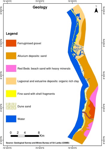
The study area is more than 48 km stretch covering the southern part of Mannar district from Vankalai to Mullikulam and is also located as a small part of the North-western coastal zone of the Gulf of Mannar in Sri Lanka. The research area is located between Latitudes 8° 34′ and 8° 56′ N and Longitudes 79° 54′ and 79° 58′ E (see part A in the Main Map). The climate in the area of study is arid, with an average rainfall of 650 mm (Miththapala, 2012). The research region comprises the two major estuaries of the Aruvi Aru and Kal Aru rivers. The Gulf of Mannar ecosystems are very rich in economically vital resources like fin fish, crustaceans, mollusks, and marine plants. It is also a habitat of the endangered dugong and marine turtles. The entire study area has Miocene sedimentary limestone bedrocks that are covered by beach deposits and alluvium (Deraniyagala, 1958; Madduma Bandara, 1989). The study area’s northern part is largely covered with fine sand deposits with shell fragments and lagoonal and estuary deposits, whereas the southern region is distinguished by fine sand deposits with shell fragments and dune sand near the shoreline (Figure 1). Although the study region is generally prograding, with rapid depositional regression, there are major concerns with coastal erosion in some areas (Miththapala, 2012). This is clearly noticeable in the study region, which is less protected from coastal currents. Some of the most affected areas by wave action are Vankalai and Chilavathurai (Madduma Bandara, 1989). Gulf of Mannar is a well-known location for marine bio-diversity and migratory birds. Vankalai is one of the prominent fishing sites in the region.

Figure 1. Geology map of the study region.

This map clearly demarcates six different types of coastal geological characteristics in the research area.

3. Materials and methods

The methodology adopted for this research to assess and monitor shoreline changes consists of three phases: (1) data acquisition, (2) demarcation of shorelines, and (3) calculation of the rate of shoreline changes (Figure 2). The shoreline changes along the study region were analyzed using Landsat satellite images from 1988, 1996, 2005, 2012, and 2022. Table 1 contains information about the data used in the analysis. The maximum cloud-free (20%) Landsat images were collected from the United States Geological Survey’s (USGS) earth explorer website (http://earthexplorer.usgs.gov), and all of them were rectified and projected with a geographical error of 0.5 pixels using the Universal Transverse Mercator System in the World Reference System WGS 1984. Using the ERDAS IMAGINE 2014 software, image pre-processing and analysis were performed. The buffering process was used to create the baseline. In a personal geo-database, all selected shorelines were merged into a single feature class. To investigate the geological and geomorphological conditions of the research location, a geological map of the study region was also obtained from the Sri Lanka Geological Survey and Mines Bureau.

Figure 2. Methodology of the study.

The data acquisition section comprises meta data information about the Landsat satellite images used in this study. The data processing section depicts the analysis procedures used prior to the shoreline analysis. The stage of analyzing data shows the hierarchical procedures required to compute shorelines changes.

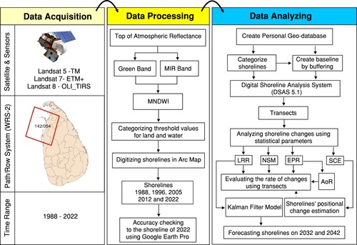
Table 1. Meta data information of the satellite imageries.

Date acquisition	Satellite & Sensor	Spatial resolution	Path/Row
1988-02-06	Landsat 5 – TM	30 m	142/54
1996-03-15	Landsat 5 – TM	30 m	142/54
2005-02-04	Landsat 5 – TM	30 m	142/54
2012-03-09	Landsat 7 – ETM+	30 m	142/54
2022-02-03	Landsat 8 – OLI_TIRS	30 m	142/54

3.1. Modified Normalized Difference Water Index (MNDWI) estimation and criteria

Several techniques for extracting coastlines and detecting changes in satellite data have been developed (Kuleli et al., 2011). However, in this study, the land and water boundaries were retrieved based on the MNDWI rate. The index of MNDWI was calculated using two spectral characteristics, such as green and middle infrared (MIR). This technique is an efficient and effective method for extracting water in general and detecting coastline in particular (Quang et al., 2021; Xu, 2018). The MNDWI is derived by Equation (1) as follows. (1) $\mathrm{M}\mathrm{N}\mathrm{D}\mathrm{W}\mathrm{I}={\displaystyle \frac{\mathrm{G}\mathrm{r}\mathrm{e}\mathrm{e}\mathrm{n}-\mathrm{M}\mathrm{I}\mathrm{R}}{\mathrm{G}\mathrm{r}\mathrm{e}\mathrm{e}\mathrm{n}+\mathrm{M}\mathrm{I}\mathrm{R}}}$(1) As a result, the MNDWI range will be used to determine the shoreline area, which reveals the border between land and water areas. The MNDWI value ranges from −1 to +1. Water pixel values must be chosen by a suitable positive threshold in order to define the water-land boundary (Kuleli et al., 2011; Weerasingha & Ratnayake, 2022).

3.2. Shoreline analysis by DSAS

The DSAS technique calculates shoreline mobility for both geographical and temporal scales using extracted shorelines (see part B in the Main Map). The transect-based method was utilized to identify shoreline change by generating perpendicular transects between the baseline and multi-temporal shoreline in the method (Quang et al., 2021). The values from the transect characteristic were employed to calculate the changes for all 836 transects that were constructed. Accuracy of the shorelines extracted from Landsat data was estimated using the most representative shoreline extracted from high-resolution image from Google Earth Pro. The shoreline (5/8/2023) extracted from the Google Earth Pro was digitized manually under 100 m eye-altitude. This shoreline was then saved in KML (Keyhole Markup Language) format and subsequently converted into layer file from Arc GIS 10.4 software. The converted layer file was exported into shape file (.shp) and saved in a personal geo-database. The shoreline dated 03/02/2022 was then merged with the shoreline extracted from Google Earth Pro and maintained in the same personal geo-database. A baseline (onshore) was also created in the personal geo-database and a transect layer was created using DSAS tool at 10-meter intervals. All the data layers were projected in Universal Transverse Mercator (WGS_1984_UTM_Zone_44N) projection and treated the attribute table with required data fields which facilitate the DSAS analysis. The statistical approaches of LRR, NSM, EPR, SCE (Shoreline Change Envelope), and AoR were used in this research. Positive accretion and negative erosion were seen in the rates of shoreline variability (Natarajan et al., 2021; Raj et al., 2020). The erosion and accretion rates for the study region were categorized into seven classes and Table 2 displays the LRR and AoR ranges (Hossen & Sultana, 2023; Margret Mary et al., 2022; Natarajan et al., 2021).

Table 2. Shoreline classifications based on erosion and accretion rates calculated by using the LRR and AoR analysis.

No	Rate of shoreline change (m/yr)	Shoreline classification
1	>−2	Very High Erosion
2	>−1 to <−2	High Erosion
3	>−1 to <0	Moderate Erosion
4	0	Stable
5	>0 to <1	Moderate Accretion
6	>1 to <2	High Accretion
7	>2	Very High Accretion

3.3. Statistical analysis

LRR portrays the rate of change statistics; slope of the line which can be evaluated by fitting the least squares regression line to all the shoreline points of a transect. The deviations were first squared, then totaled up. There are no cancellations between positive and negative readings. The explanatory variable (x) is the coastline date in years, and the dependent variable (y) is the distance from the baseline in meters calculated by the Equation (2). As a result, the linear regression rate corresponds to the slope of the line (Himmelstoss et al., 2018). The entire computational process was very simple and it was a widely proven statistical concept (Crowell et al., 1997; Dolan et al., 1991b). LRR is the most appropriate method to predict the future shoreline position and their associated confidence intervals, if measurement errors and a linear trend of erosion were the only determining factors over the longest possible periods of shoreline position (Crowell et al., 1997; Douglas & Crowell, 2000). (2) $LRR={\displaystyle \frac{\left(\delta y-c\right)}{\delta x}}$(2) The NSM and the time interval between the oldest and most current coastline were divided to obtain the analytical rate of EPR (Natarajan et al., 2021). The merit of EPR was relatively easy to compute and it needs two shoreline dates at a minimum, calculated by the Equation (3). The demerits of EPR when more data are available, the additional information is ignored such as changes in sign (i.e.) erosion and accretion, magnitude or cyclical trends may be missed (Himmelstoss et al., 2018). (3) $EPR=\left\{{\displaystyle \frac{d_{2022}-d_{1988}}{t_{2022}-t_{1988}}}\right\}m/year$(3) Calculated EPRs were further used to estimate the Average of Rate (AoR) for better interpretation of the rates (Equation (4)) where n is number of cases (or number of EPRs) as described by Dolan et al., (1991a). (4) $AoR={\displaystyle \frac{{\sum }_{i=1}^{n}EPR}{n}}$(4) Minimum time (T_min) required to calculate the AoR was also estimated using Equation (5) to check whether the time intervals of the shorelines are acceptable or not for this calculation (Deepika et al., 2014; Dolan et al., 1991a). (5) $T_{min}={\displaystyle \frac{\sqrt{E{1}^2+E{2}^2}}{R1}}$(5) where E1 (15 m) and E2 (15 m) are the measurement errors of first and second shoreline points. R1 is the EPR of the transect and T_min is the minimum required time interval. Measurement error was used as 15 m because the geographical error in the rectified images is 0.5 pixels (or 15 m).

For each transect or hypothetical line that crosses a shoreline perpendicularly, the NSM Equation (6) below summarizes the actual distance between the oldest and youngest shoreline (Chrisben Sam & Gurugnanam, 2022; Natarajan et al., 2021). (6) $\mathrm{N}\mathrm{S}\mathrm{M}=\left\{d_{1988}-d_{2022}\right\}m$(6) Positional change of the shoreline delineated from the Landsat data compared to the shoreline delineated from the Google Earth Pro was estimated using SCE statistics in DSAS tool. SCE is a measurement of the overall change in shoreline movement that takes into account all viable shoreline positions and reports their distances without making particular references to their specific dates (Himmelstoss et al., 2018). Mean SCE (after removing the outliers) was used as the uncertainty of the digitized shorelines from Landsat data compared to the high-resolution data in Google Earth Pro.

3.4. Prediction of future shorelines by Kalman filter model

The prediction of future shoreline trends is the most challenging and significant factor in coastal management planning (Abdul Maulud et al., 2022). The prediction of long-term shoreline changes is quite difficult due to its dynamic state on the earth’s surface (Ciritci & Türk, 2019). (Yates et al., 2009) derived the equations (7, 7a) for determining the total shoreline position and its change. $X\left(t\right)=X_{{}_{lt}}\left(t\right)+X_{st}\left(t\right)$ (7) ${\displaystyle \frac{dX}{dt}=v_{lt}+C{E}^{1/2}\mathrm{\Delta }E\left(7\mathrm{a}\right)}$(7) where as $X$_lt – shoreline change; $X$_{st –} shorter term shoreline response; $v_{lt}$ _– long-term rate of shoreline change position; $C{E}^{1/2}$ – shoreline change induced by waves; $\mathrm{\Delta }E$ – wave energy disequilibrium

In this study, prediction and forecasting were achieved using an advanced extrapolation method called Kalman filter model algorithm in (DSAS v 5.1) plugin. The Kalman filter method is a recursive algorithm that applies many stages to estimations of the current state variable, which is the main distinction between it and simple extrapolation (Islam & Crawford, 2022). This algorithm calculates the estimates of some unknown variables given the measurements observed over the period of time. (Kim & Bang, 2019) stated that Kalman filter model comprises two phases such as prediction and updation. In general, Kalman filter algorithm was defined by the Equations (8, 9) as follows. (8) ${\hat{x}}_k^{-}=F{\hat{x}}_{k-1}^{+}+B{u}_{k-1}$(8) (9) $P_K^{-}=F{P}_{K-1}^{+}{F}^T+Q$(9) In the above equations,

• ^ – estimate of a variable

• Superscripts (+ and −) – predicted and updated estimates

• P – state of error covariance

• T – duration

• Q – (covariance of noise) are constant

• F_k – state transition model which is applied to the previous state x_k-1

• B_k - control-input model which is applied to the control vector u_k-1

The DSAS (v. 5.1) tool includes an integrated Kalman filter model algorithm to evaluate the coastline position for more than 10 and 20 years in the future. This evaluation was based on the historical shoreline position (1988, 1996, 2005, 2012, and 2022). This statistical tool was initialized by the LRR calculated by DSAS (Long & Plant, 2012). LRR values act as preliminary data for calculating the next 2032 and 2042 shoreline trends with uncertainty band. Once the shoreline position was encountered, Kalman filter algorithm plays a vital role in minimizing the error between both modeled and observed shoreline position to enhance the forecast, with updated rates and uncertainties (Ciritci & Türk, 2020; Natarajan et al., 2021). The updated rates act as a major key factor for predicting the shoreline position until the desired time period is met (Chrisben Sam & Gurugnanam, 2022; Himmelstoss et al., 2018). Therefore, 2032 and 2042 shoreline trends were predicted using Kalman filter model to the study region for the forecasting.

4. Results

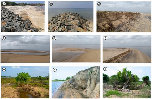
Line charts in the Main Map part C (1), (2), and (3) show the statistics of erosion and deposition rates corresponding to all LRR, EPR, and NSM transects obtained in this coastal analysis. Mean uncertainty of the shorelines extracted from Landsat data is estimated as 25.86 ± 16.7 m. For easier analysis and evaluation, we split the study region into four main sectors: Vanchiyankulam, Aruvi Aru, Palsotikandal, and Karadikkuli. Furthermore, estimated AoR was used in conjunction with LRR to interpret the rate of change as AoR satisfied the minimum time interval for the EPR estimate. AoR and LRR values reflect the rate of erosion and accretion during the time period of 1988–2022. The LRR values depict that the maximum erosion rate was observed −4.7 m/year at Vankalai west and Naruvilikulam situated in Vankalai sector and the maximum accretion rate was 10.3 m/year at Ferry in Aruvi Aru sector (see part D (1) in the Main Map). The AoR clearly portrays that the values are indistinguishable, highest erosion (−5.3 m/year) and the maximum accretion (9.6 m/year) in the same sectors (see part D (2) in the Main Map). The NSM values exhibit that the shoreline was retreated by 194.8 m at Vankalai, Umanagiri, and Kondachchikudah and the shoreline encroached by sediments at the rate of 370.7 m in Pampaditta Odai, Achchankulam and Ferry over the period of time (see part D (3) in the Main Map). Based on the existing values of AoR and LRR the accretion also took place in Pampaditta Odai, Karadikkuli, Mutharipputhurai, and Achchankulam whereas the erosion of shorelines occurs in Kalapuwa, Umanagiri, Pathaikaddumunai, Kayakuli, and Mallikannaddi. Figure 3 shows the field evidence related to erosion and accretion due to natural and anthropogenic activities that took place in the hotspots of the study area.

Figure 3. The field study photographs A-B-C-D-E-F-G-H-I show some natural processes and human activities which are related to the accretion and erosion in the study area.

Read the detailed description of this figure

A- illustrates a section of the eroding coastal site in Vankalai area in the study region. The scene shows the sea waves are being eroded more towards the land area from sea. B- Human activity depicts a view of a stone fence placed on the shore in Vankalai area to protect against the sea waves and currently being covered by sea water. C- describes the eroded of coastal sandy soils due to the impact of sea waves in Vankalai area. D- highlights the barrier-built formation that has occurred in the estuary transition zone of Aruvi Aru due to the deposition of their increased sediment load. E- indicates a small spit formation at the Aruvi Aru estuary near to Arippu area in the study region. F- refers the area of sediment which has accumulated in the Kal Aru estuary. G- The photo describes an illegal sand mining activity near the Aruvi Aru river flood plain. The activity may extend in the future and affecting the neighboring mangroves associates patches as well. H- The photograph depicts the retreating river bank due to increased flood levels and runoff near the Aruvi Aru estuary. It is a high risk for sediment deposition at the river mouth due to this eroding process. I- highlights the scene where nearby a tree collapsed due to the increased sand mining activity which occurred near to the estuary of Kal Aru river.

5. Discussion

5.1. Vanchiyankulam sector

This sector was mainly governed by erosion and in some regions moderate accretion was observed. This is mainly due to the North-West monsoon wind towards the coastal zone of Vankalai region, whereas the direction and the velocity of the wind play a vital role in determining the coastal erosion in this sector. The maximum erosion rate was −4.3 (LRR & AoR) m/year at Vankalai. NSM estimated that erosion of 147.9 m at Vankalai and Umanagiri and 59 m at Kalapuwa. Mostly this sector experiences very high erosion to high erosion (−3.2 to −2.5 m/year) in Vankalai, Mallikannaddi, and Naruvilikulam.

5.2. Aruvi Aru sector

This sector experiences very high accretion while compared to erosion. Historical landmarks such as Arippu Dutch Fort and Doric Bangalow are the most significant hotspots in this sector. The maximum rate of erosion were −4.4 m/year (LRR) and −5.3 m/year (AoR) at Pathaikaddumunai and maximum rates of accretion were 8.8 m/year (LRR) and 9.6 m/year (AoR). The NSM values showed that the shoreline retreated by 194 m in Pathaikaddumunai and Kailikulam and advanced by 370 m in Kannaditivu, Ferry and Kulankulam. Illegal sand mining in Aruvi Aru is the major reason for costal accretion, whereas spits and barriers act as major geomorphological features for very high accretion in this sector.

5.3. Palsotikandal sector

This sector is subjected to both erosion and accretion. It has costal alluvium and sand wash deposits and comprises of small villages such as Kokkappadayan, Kondachchikudah, Pampaditta Odai, and Kayakuli. Kondachchikudah experiences very high erosion at the rate of – 4.8 (LRR) and 5.2 (AoR). Southwest monsoon wind plays a significant role in erosion and it resembles like a concave structure. Likewise, Pampaditta Odai and Kayakuli fishing huts encountered a very high accretion at the rate of 10.3 m/year (LRR & AoR). The high accretion in Pampaditta Odai is due to the input of sediment load in Kal Aru estuary. The NSM values show that the shoreline retreated by 173 m at Kondachchikudah and advanced by 350 m at Pampaditta Odai. Moderate to high accretion was recorded in Kokkuppadayan and Kayakuli at the rate of 0.01–1.62 m/year.

5.4. Karadikkuli sector

Rate of accretion is more dominant compared to erosion. This sector comprises of small villages such as Kallaru, Vannamoddai, and Koraimoddai. Kallaru river flows through this sector and it acts as natural agent for transporting the sediments load. The maximum rate of erosion were 1.8 m/year both in LRR and AoR Koraimoddai and the maximum rate of accretion were 1.2 m/year (LRR) and 1.8 m/year (AoR) near Karadikuli, Vannamoddai, and Marthondikudah. The shoreline was advanced at the rate of 31.5 m in Udumbupidiththaveli, Karadikuli, Vannamoddai, and Marthondikudah and retreated at the rate of 24.5 m in Koraimoddai. The elevation of this sector was relatively high while compared to other sectors, due to the coarse of elevation the sediment load from Kallaru gets accumulated.

5.5. Forecasting and prediction shorelines for 2032 and 2042

In this study, Kalman filter model was used for predicting the future shoreline trends of 2032 and 2042 periods. In addition to that we have estimated that eight different zones have possibilities for severe erosion and accretion in future. We estimated that by 2032, Vankalai’s shoreline would have significantly eroded by about 15 m, and Pathaikaddumunai’s shoreline might have been deposited by about 25 m. By 2042, Vankalai’s shoreline could have further eroded by about 45 m, and Pathaikaddumunai’s shoreline might have deposited by a maximum of 78 m. In continuation of shoreline erosion in Vankalai over the next two decades suggest that the South-west monsoon wind direction and its velocity continue to increase. We also expect that the shorelines at Mallikannadi, Arippu, and Kondachikudah would experience erosion until 2042 (see part E in the Main Map).

The accuracy assessment implies that the shoreline positional error is comparatively high as it is around 25 m. The main reason for this estimation is the limited spatial resolution (30 m) of Landsat data. However, Landsat data are effective in terms of its temporal resolution so that it is important to use Landsat data for shoreline change analysis at the places where the change is more than 25 m (as per the accuracy assessment). In addition, tidal actions, seasonal variations, and sea level rise can be influenced on this uncertainty too. But, they were not taken into consideration as it is comparatively low considering the effect from the spatial resolution of the images. By considering all these aspects, the overall study interprets the accretion and erosion natures of the shorelines at the places where the NSM values are greater than 25 m.

6. Conclusion

Shoreline evolution between Aruvi Aru and Kal Aru coastal stretch on the north-western coastal zone in Mannar district, Sri Lanka was effectively demarcated and analyzed between 1988 and 2022 frames, utilizing GIS techniques and automatic computations using DSAS. Using multi-temporal satellite images acquired over a 34-year period, shoreline evolution detection along the coastline stretch was extensively investigated (between 1988 and 2022). The analysis revealed that some of the evaluated areas were experiencing significant erosion. The research area’s northern part has mainly experienced considerable rates of erosion. Vankalai and Kondachikudah, as well as the areas around them, should be designated as high erosion risk zones based on the estimated results. The areas around the estuaries of the Aruvi Aru and Kal Aru are also where massive accretion was most observable. Several factors have been identified as contributing to the erosion in the study site, including the south-west monsoon season’s high wave action, the topography of the area, and the geomorphological and geological conditions. It can be seen that accretion processes are taking place due to the natural flows of the major rivers in the study area and also due to the activities of illegal sand mining in the respective rivers. On the other side, the Kalman filter model projected the futuristic shoreline to 2032 and 2042. Ultimately, the prediction model revealed that the shoreline position will continue to shift landward in the future. Increasing Vankalai area’s coastal erosion may put the adjacent Aruvi Aru estuary and its surrounding ecosystems under threat in future. However, the findings of this study can be implemented to the sustainability of coastal zone management and the development of suitable coastal design of structures throughout Sri Lanka’s north-western coastal zone. There is no doubt that the findings of this study will help future coastal zone planners to protect areas threatened by coastal erosion and sedimentation problems in Sri Lanka.

Therefore, there is a need to emphasize the limitations and future research directions of this shoreline study. The utilization of 30 m resolution Landsat images may have introduced certain constraints and influenced the accuracy of the findings. Future studies could explore the integration of other data sources, such as aerial imagery or Light Detection and Ranging (LiDAR) data, to improve the accuracy of shoreline mapping and change detection. Additionally, advances in satellite technology may offer higher-resolution imagery in the future, enabling more detailed and precise analyses. Despite these limitations, this study serves as a valuable foundation for future research in this field. By establishing a baseline understanding of the shoreline dynamics, it provides a starting point for more detailed investigations using higher-resolution imagery or alternative remote sensing techniques. The findings and insights gained from this study can guide future researchers in designing and implementing more comprehensive studies.

Software

ERDAS IMAGINE 2014 software is used for image processing analysis, while Arc GIS 10.4 was used for DSAS analysis and the preparation of basic layout maps.

Disclosure statement

No potential conflict of interest was reported by the author(s).

Data availability statement

This analysis used multi-spectral Landsat imageries. These images were downloaded from the Earth Explorer site of the USGS website, which is available at http://earthexplorer.usgs.gov/. It is possible to share the vector data for the shorelines and transects that were measured using the DSAS tool when needed.

References

- Abdul Maulud, K. N., Selamat, S. N., Mohd, F. A., Md Noor, N., Wan Mohd Jaafar, W. S., Kamarudin, M. K. A., Ariffin, E. H., Adnan, N. A., & Ahmad, A. (2022). Assessment of shoreline changes for the Selangor Coast, Malaysia, using the digital shoreline analysis system technique. Urban Science, 6(4), 71. https://doi.org/10.3390/urbansci6040071
- Allan, J. C., Komar, P. D., & Priest, G. R. (2003). Shoreline variability on the high-energy Oregon coast and its usefulness in erosion-hazard assessments. Journal of Coastal Research, 83–105.
- Al-Zubieri, A. G., Ghandour, I. M., Bantan, R. A., & Basaham, A. S. (2020). Shoreline evolution between Al Lith and Ras Mahāsin on the Red Sea Coast, Saudi Arabia using GIS and DSAS techniques. Journal of the Indian Society of Remote Sensing, 48(10), 1455–1470. https://doi.org/10.1007/s12524-020-01169-6
- Azhar, M. M., Maulud, K. N. A., Selamat, S. N., Khan, M. F., Jaafar, O., Jaafar, W. S. W. M., Abdullah, S. M. S., Toriman, M. E., Kamarudin, M. K. A., Gasim, M. B., & Juahir, H. (2018). Impact of shoreline changes to the coastal development. International Journal of Engineering & Technology, 7(3.14), 191–195. https://doi.org/10.14419/ijet.v7i3.14.16883
- Chen, L., Wang, X., Cai, X., Yang, C., & Lu, X. (2022). Seasonal variations of daytime land surface temperature and their underlying drivers over Wuhan, China. Remote Sensing, 14(2), 1–22. https://doi.org/10.3390/rs14010001
- Chrisben Sam, S., & Gurugnanam, B. (2022). Coastal transgression and regression from 1980 to 2020 and shoreline forecasting for 2030 and 2040, using DSAS along the southern coastal tip of Peninsular India. Geodesy and Geodynamics, 13(6), 585–594. https://doi.org/10.1016/j.geog.2022.04.004
- Ciritci, D., & Türk, T. (2019). Automatic detection of shoreline change by geographical information system (GIS) and remote sensing in the Göksu Delta, Turkey. Journal of the Indian Society of Remote Sensing, 47(2), 233–243. https://doi.org/10.1007/s12524-019-00947-1
- Ciritci, D., & Türk, T. (2020). Assessment of the Kalman filter-based future shoreline prediction method. International Journal of Environmental Science and Technology, 17(8), 3801–3816. https://doi.org/10.1007/s13762-020-02733-w
- Crowell, M., Douglas, B. C., & Leatherman, S. P. (1997). A test of algorithms. Source: Journal of Coastal Research Journal of Coastal Research, 13(4), 1245–1255. http://www.jstor.org/stable/4298734%5Cnhttp://about.jstor.org/terms
- Dastgheib, A., Jongejan, R., Wickramanayake, M., & Ranasinghe, R. (2018). Regional scale risk-informed land-use planning using Probabilistic Coastline Recession modelling and economical optimisation: East Coast of Sri Lanka. Journal of Marine Science and Engineering, 6(4), 120–132. https://doi.org/10.3390/jmse6040120
- Dede, M., Susiati, H., Widiawaty, M. A., Kuok-Choy, L., Aiyub, K., & Asnawi, N. H. (2023). Multivariate analysis and modeling of shoreline changes using geospatial data. Geocarto International, 38(1). https://doi.org/10.1080/10106049.2022.2159070
- Deepika, B., Avinash, K., & Jayappa, K. S. (2014). Shoreline change rate estimation and its forecast: Remote sensing, geographical information system and statistics-based approach. International Journal of Environmental Science and Technology, 11(2), 395–416. https://doi.org/10.1007/s13762-013-0196-1
- Deraniyagala, P. E. P. (1958). The Pleistocene of Ceylon. Ceylon National Museums Natural History Series.
- Dewi, R. S., & Bijker, W. (2020). Dynamics of shoreline changes in the coastal region of Sayung, Indonesia. The Egyptian Journal of Remote Sensing and Space Science, 23(2), 181–193. https://doi.org/10.1016/j.ejrs.2019.09.001
- Dolan, R., Fenster, M. S., & Holme, S. J. (1991a). Florida accretion. Journal of Coastal Research, 7(3), 723–744.
- Dolan, R., Fenster, M. S., & Holme, S. J. (1991b). Temporal analysis of shoreline recession and accretion. Journal of Coastal Research, 7, 723–744.
- Douglas, B. C., & Crowell, M. (2000). Long-term shoreline position prediction and error propagation. Journal of Coastal Research, 16, 145–152.
- Himmelstoss, E. A., Henderson, R. E., Kratzmann, M. G., & Farris, A. S. (2018). Digital Shoreline Analysis System (DSAS) Version 5.0 User Guide. U.S. Geological Survey Open-File Report 2021–1091, 1–104.
- Hossen, M. F., & Sultana, N. (2023). Shoreline change detection using DSAS technique: Case of Saint Martin Island, Bangladesh. Remote Sensing Applications: Society and Environment, 30, 100943. https://doi.org/10.1016/j.rsase.2023.100943
- Islam, M. S., & Crawford, T. W. (2022). Assessment of spatio-temporal empirical forecasting performance of future shoreline positions. Remote Sensing, 14(24), 6364. https://doi.org/10.3390/rs14246364
- Kim, Y., & Bang, H. (2019). Introduction to Kalman filter and its applications. Introduction and Implementations of the Kalman Filter, 1–16. https://doi.org/10.5772/intechopen.80600
- Kottawa-Arachchi, J. D., & Wijeratne, M. A. (2017). Climate change impacts on biodiversity and ecosystems in Sri Lanka: A review. Nature Conservation Research, 2(3), 2–22. https://doi.org/10.24189/ncr.2017.042
- Kuleli, T., Guneroglu, A., Karsli, F., & Dihkan, M. (2011). Automatic detection of shoreline change on coastal Ramsar wetlands of Turkey. Ocean Engineering, 38(10), 1141–1149. https://doi.org/10.1016/j.oceaneng.2011.05.006
- Kundu, S., Mondal, A., Khare, D., Mishra, P. K., & Shukla, R. (2014). Shifting shoreline of Sagar Island Delta, India. Journal of Maps, 10(4), 612–619. https://doi.org/10.1080/17445647.2014.922131
- Long, J. W., & Plant, N. G. (2012). Extended Kalman Filter framework for forecasting shoreline evolution. Geophysical Research Letters, 39(13), 1–6. https://doi.org/10.1029/2012GL052180
- Luijendijk, A., Hagenaars, G., Ranasinghe, R., Baart, F., Donchyts, G., & Aarninkhof, S. (2018). The state of the world’s beaches. Scientific Reports, 8(1), 1–12. https://doi.org/10.1038/s41598-018-24630-6
- Madduma Bandara, C. M. (1989). A survey of the coastal zone of Sri Lanka. Coast Conservation Department.
- Maiti, S., & Bhattacharya, A. K. (2009). Shoreline change analysis and its application to prediction: A remote sensing and statistics based approach. Marine Geology, 257(1-4), 11–23. https://doi.org/10.1016/j.margeo.2008.10.006
- Margret Mary, G., Sundar, V., & Sannasiraj, V. A. S. (2022). Analysis of shoreline change between inlets along the coast of Chennai, India. Marine Georesources & Geotechnology, 40(1), 26–35. https://doi.org/10.1080/1064119X.2020.1856241
- Mehvar, S., Dastgheib, A., Bamunawala, J., Wickramanayake, M., & Ranasinghe, R. (2019). Quantitative assessment of the environmental risk due to climate change-driven coastline recession: A case study in Trincomalee coastal area, Sri Lanka. Climate Risk Management, 25, 100192. https://doi.org/10.1016/j.crm.2019.100192
- Miththapala, S. (2012). The Gulf of Mannar and its surroundings: A resource book for teachers in the Mannar District.
- Mohd, F. A., Maulud, K. N. A., Begum, R. A., Selamat, S. N., & Karim, O. A. (2018). Impact of shoreline changes to pahang coastal area by using geospatial technology. Sains Malaysiana, 47(5), 991–997. https://doi.org/10.17576/jsm-2018-4705-14
- Moussaid, J., Fora, A. A., Zourarah, B., Maanan, M., & Maanan, M. (2015). Using automatic computation to analyze the rate of shoreline change on the Kenitra coast, Morocco. Ocean Engineering, 102, 71–77. https://doi.org/10.1016/j.oceaneng.2015.04.044
- Nandi, S., Ghosh, M., Kundu, A., Dutta, D., & Baksi, M. (2016). Shoreline shifting and its prediction using remote sensing and GIS techniques: A case study of Sagar Island, West Bengal (India). Journal of Coastal Conservation, 20(1), 61–80. https://doi.org/10.1007/s11852-015-0418-4
- Nassar, K., Mahmod, W. E., Fath, H., Masria, A., Nadaoka, K., & Negm, A. (2019). Shoreline change detection using DSAS technique: Case of North Sinai coast, Egypt. Marine Georesources & Geotechnology, 37(1), 81–95. https://doi.org/10.1080/1064119X.2018.1448912
- Natarajan, L., Sivagnanam, N., Usha, T., Chokkalingam, L., Sundar, S., Gowrappan, M., & Roy, P. D. (2021). Shoreline changes over last five decades and predictions for 2030 and 2040: A case study from Cuddalore, southeast coast of India. Earth Science Informatics, 14(3), 1315–1325. https://doi.org/10.1007/s12145-021-00668-5
- Nithu Raj, G. B., Sudhakar, V., & Glitson Francis, P. (2019). Estuarine shoreline change analysis along The Ennore river mouth, south east coast of India, using digital shoreline analysis system. Geodesy and Geodynamics, 10(3), 205–212. https://doi.org/10.1016/j.geog.2019.04.002
- Oyedotun, T. D. T. (2014). Shoreline geometry : DSAS as a tool for historical trend analysis. In Geomorphological techniques (online edition) (Vol. 2, pp. 1–12). London, UK: British Society for Geomorphology.
- Palamakumbure, L., Ratnayake, A. S., Premasiri, H. M. R., Ratnayake, N. P., Katupotha, J., Dushyantha, N., Weththasinghe, S., & Weerakoon, W. A. P. (2020). Sea-level inundation and risk assessment along the south and southwest coasts of Sri Lanka. Geoenvironmental Disasters, 7(1), https://doi.org/10.1186/s40677-020-00154-y
- Quang, D. N., Ngan, V. H., Tam, H. S., Viet, N. T., Tinh, N. X., & Tanaka, H. (2021). Long-term shoreline evolution using DSAS technique: A case study of Quang Nam province, Vietnam. Journal of Marine Science and Engineering, 9(10), 1124. https://doi.org/10.3390/jmse9101124
- Raj, N., Rejin Nishkalank, R. A., & Chrisben Sam, S. (2020). Coastal shoreline changes in Chennai: Environment impacts and control strategies of Southeast Coast, Tamil Nadu. Handbook of Environmental Materials Management, 1–14. https://doi.org/10.1007/978-3-319-58538-3_223-1
- Ratnayakage, S. M. S., Sasaki, J., Suzuki, T., Jayaratne, R., Ranawaka, R. A. S., & Pathmasiri, S. D. (2020). On the status and mechanisms of coastal erosion in Marawila Beach, Sri Lanka. Natural Hazards, 103(1), 1261–1289. https://doi.org/10.1007/s11069-020-04034-4
- Roy, S., Mahapatra, M., & Chakraborty, A. (2018). Shoreline change detection along the coast of Odisha, India using digital shoreline analysis system. Spatial Information Research, 26(5), 563–571. https://doi.org/10.1007/s41324-018-0199-6
- Senevirathna, E. M. T. K., Edirisooriya, K. V. D., Uluwaduge, S. P., & Wijerathna, K. B. C. A. (2018). Analysis of causes and effects of coastal erosion and environmental degradation in Southern Coastal Belt of Sri Lanka special reference to Unawatuna Coastal Area. Procedia Engineering, 212, 1010–1017. https://doi.org/10.1016/j.proeng.2018.01.130
- Warnasuriya, T. W. S., Gunaalan, K., & Gunasekara, S. S. (2018). Google earth: A new resource for shoreline change estimation – case study from Jaffna Peninsula, Sri Lanka. Marine Geodesy, 41(6), 546–580. https://doi.org/10.1080/01490419.2018.1509160
- Weerasingha, W. A. D. B., & Ratnayake, A. S. (2022). Coastal landform changes on the east coast of Sri Lanka using remote sensing and geographic information system (GIS) techniques. Remote Sensing Applications: Society and Environment, 26, 100763. https://doi.org/10.1016/j.rsase.2022.100763
- Wong, P. P., Losada, I. J., Gattuso, J. P., Hinkel, J., Khattabi, A., McInnes, K. L., Saito, Y., Sallenger, A., Nicholls, R. J., Santos, F., & Amez, S. (2014). Coastal systems and low-lying areas. In Climate Change 2014 Impacts, Adaptation and Vulnerability: Part A: Global and Sectoral Aspects (Issue October). https://doi.org/10.1017/CBO9781107415379.010
- Xu, N. (2018). Detecting coastline change with all available landsat data over 1986-2015: A case study for the state of Texas, USA. Atmosphere, 9(3), 107. https://doi.org/10.3390/atmos9030107
- Yan, D., Yao, X., Li, J., Qi, L., & Luan, Z. (2021). Shoreline change detection and forecast along the Yancheng Coast using a digital shoreline analysis system. Wetlands, 41(4). https://doi.org/10.1007/s13157-021-01444-3
- Yates, M. L., Guza, R. T., & O’Reilly, W. C. (2009). Equilibrium shoreline response: Observations and modeling. Journal of Geophysical Research: Oceans, 114(9), 1–16. https://doi.org/10.1029/2009JC005359