A new model for cloud elastic services efficiency

ABSTRACT

The speedup measures the improvement in performance when the computational resources are being scaled. The efficiency, on the other side, provides the ratio between the achieved speedup and the number of scaled computational resources (processors). Both parameters (speedup and efficiency), which are defined according to Amdahl’s Law, provide very important information about performance of a computer system with scaled resources compared with a computer system with a single processor. However, as cloud elastic services’ load is variable, apart of the scaled resources, it is vital to analyse the load in order to determine which system is more effective and efficient. Unfortunately, both the speedup and efficiency are not sufficient enough for proper modeling of cloud elastic services, as the assumptions for both the speedup and efficiency are that the system’s resources are scaled, while the load is constant. In this paper, we extend the scaling of resources and define two additional scaled systems by (i) scaling the load and (ii) scaling both the load and resources. We introduce a model to determine the efficiency for each scaled system, which can be used to compare the efficiencies of all scaled systems, regardless if they are scaled in terms of load or resources. We have evaluated the model by using Windows Azure and the experimental results confirm the theoretical analysis. Although one can argue that web services are scalable and comply with Gustafson’s Law only, we provide a taxonomy that classifies scaled systems based on the compliance with both the Amdahl’s and Gustafson’s laws.

For three different scaled systems (scaled resources R, scaled load L and combination RL), we introduce a model to determine the scaling efficiency. Our model extends the current definition of efficiency according to Amdahl’s Law, which assumes scaling the resources, and not the load. $$\begin{array}{c}\hfill E_R=\frac{S_R}{p}=\frac{T(1)}{T_R}·\frac{1}{p};E_L=S_L·N=\frac{T(1)}{T_L}·N;E_{\mathit{RL}}=S_{\mathit{RL}}·\frac{N}{p}=\frac{T(1)}{T_{\mathit{RL}}}·\frac{N}{p}\end{array}$$

GRAPHICAL ABSTRACT

KEYWORDS:

• Efficiency
• load
• optimisation
• performance
• resources
• speedup

1. Introduction

Cloud computing has profoundly influenced the architecture design of the concurrent distributed systems, thus allowing transition from license-based to as-a-service-based services [1]. Essentially, customers are not required to purchase specific licenses to own the software services, instead, they can use it and pay for the period of its usage only. The main enablers of the recent advances in service provisioning can be identified in the improved on-demand elastic resource scaling. Cloud providers currently offer various types of physical resources in the form of virtual machine (VM) instances, each one with specific computing, memory and storage capacity. Moreover, to satisfy the customers’ demands, the leased resources can be easily scaled horizontally, that is, scaled out or scaled in, or vertically, i.e. scaled up or scaled down. Due to its high elasticity and the linear pay-as-you-go business model, the cloud is a preferred platform for various types of applications. It can yield significant performance and financial benefits, especially for low-communication services, such as scientific applications [2,3]. However, there is a wide set of communication-intensive applications, which are not suitable for the loosely coupled cloud infrastructure and can not easily benefit from it. The heterogeneity and the wide geographical distribution of the cloud platforms can become a significant drawback, primarily due to the limited communication performance between the computing nodes [4].

Despite the cloud’s elasticity, the customers are concerned about its scalability, that is, whether they will achieve a proportional performance to the leased resources. In order to comply with the guaranteed quality of service (QoS), cloud customers usually rent more resources than necessary to speed up their services or to handle more requests in a proper time. The achieved speedup, still, shows the effectiveness of adding more resources, without showing how much efficient they are.

Many definitions of efficiency can be found in the literature. For example, achieved performance compared to the peak for some period of time [5], or consumed resources to process some amount of work [6]. Chen et al. [7] define the power efficiency of a cloud as a measure how the consumed power is used. In this paper, we focus on the classical efficiency definition according to Amdahl’s Law [8], which calculates it as a ratio between the achieved improvement in speedup and the scaled (increased) resources. Although this is a very important parameter for cloud elastic resources, still, it does not show how efficient will be the given resource if the load is scaled (either increased or decreased).

For example, let us assume that a service is deployed in a VM in the cloud and it provides a response time of $10\mathrm{\mu }$s when loaded with 1 request per second (non-Scaled case). Let us consider two scaled cases (S5 and S100), for which the load is increased to 5 and 100 requests per second, correspondingly, that is, the resources are scaled five and 100 times compared to the non-Scaled case. Most probably, the total execution time for the S5 case will be in the range from $1·10\mathrm{\mu }$s up to $5·10\mathrm{\mu }$s, since the server is underutilised. On the other hand, in the S100 case, the server will be overutilised, and the total execution time will be greater than $100·10\mathrm{\mu }\text{s}=1000\mathrm{\mu }$s. Without loosing generality, let us assume that the total execution time for S5 case will be $30\mathrm{\mu }$s, while for the S100 case will be 5 s. For both cases, underutilisation or overutilisation, the current definitions of efficiency will not provide any useful information. Indeed, the achieved speedup (slowdown in this case) will be $10\mathrm{\mu }\text{s}/30\mathrm{\mu }\text{s}=0.33$ for the scaled S5 case, while even much smaller speedup (greater slowdown) will be achieved for the S100 case, i.e. $10\mathrm{\mu }\text{s}/5\text{s}=2·{10}^{-6}$. Further on, both scaled cases S5 and S100 will have the same ratio of efficiency, as both cases use the same resources (let us assume 1). Therefore, the efficiency will be 0.33 and $2·{10}^{-6}$, correspondingly.

Using this example, we show two weaknesses of current definition of the efficiency. Firstly, both cases S5 and S100 use the same resources as the original non-Scaled case and therefore, their efficiencies are proportional and depend directly on the speedup only. Secondly, it is obvious that the S5 case achieves the greatest speed of 1 / 6 request per $\mathrm{\mu }$s (166 requests per ms) and therefore, it should be more efficient than the original non-Scaled case’s speed of 1 / 10 request per $\mathrm{\mu }$s (100 requests per ms).

For this purpose, in this paper, we introduce a model to determine the appropriate speedup and efficiency of scaling for three different scaled systems (scaled resources, scaled load and their combination). We argue that, apart of the speedup and resources, it is necessary to include the load, as well, in the efficiency definition, especially for the elastic cloud services. Our model is evaluated with real world application executed in Windows Azure Cloud that utilises several cloud’s services. This paper significantly extends our previous research [9], where we model several performance indicators, to determine which law (the Amdahl’s or Gustafson’s [10]) holds for the cloud elastic services, and in which specific ratio between problem size and resources. Although one would expect that scalable web services may comply with the Gustafson’s law only, we introduce a new taxonomy that classifies the scaled systems complying with both the Amdahl’s and Gustafson’s laws.

The rest of the paper is organised as follows. The background of the basic metrics that describe the parallel and distributed systems are described in Section 2. Our motivation to revise the efficiency definition and to develop a new model and taxonomy for cloud elastic services is elaborated in Section 3. Section 4 defines the new developed taxonomy for scaled systems in the cloud and presents the theoretically expected performance. According to the taxonomy, Section 5 models the speedup and introduces efficiency for each scaled system by considering various load regions. The correctness of the model is evaluated and discussed in Section 6. Section 7 compares our results with related work. Finally, we conclude the paper and present the plans for future work in Section 8.

2. Background

In this section, we present the basic metrics that are used most often to describe a parallel and distributed system in terms of performance. The section also presents the speedup and efficiency limits according to the Amdahl’s and Gustafson’s laws.

Parallel and distributed systems offer a powerful environment that can be utilised for two main purposes: to speed up some algorithm’s execution or to execute big data problems. The former is useful in order to complete the execution in a limited time constraint, for example, obtaining the simulation results for today’s weather forecast in the following day is totally unacceptable and unusable. Distributed systems are used to solve a problem that cannot be even started on a single machine due to hardware limitations. Both the parallel and distributed systems have more computing resources than a nominal (non-scaled) single-machine or a single-processor system. In this paper, we will denote these systems as scaled systems.

2.1. Modeling the performance of a system with scaled resources

Let’s analyse a scaled system with n processors (or computing resources). The metric for measuring the performance of a scaled computing system is the speed V(n), which defines the amount of work W(n) performed for a period of time T(n), as presented in (1(1) $$\begin{array}{c}\hfill V(n)=\frac{W(n)}{T(n)}\end{array}$$(1) ).(1) $$\begin{array}{c}\hfill V(n)=\frac{W(n)}{T(n)}\end{array}$$(1)

Another important metric is the normalised speed NV(n), defined as achieved speed per processor, which measures the average amount of work per processor per time period, as defined in (2(2) $$\begin{array}{c}\hfill NV(n)=\frac{V(n)}{n}=\frac{W(n)}{n·T(n)}\end{array}$$(2) ).(2) $$\begin{array}{c}\hfill NV(n)=\frac{V(n)}{n}=\frac{W(n)}{n·T(n)}\end{array}$$(2)

The normalised speed NV(n) assumes a homogeneous environment where all processors are the same. Nevertheless, each processor usually does not finish the assigned work at the same time and most of them will provide a slack time since the work usually cannot be divided evenly. Therefore, all processors will wait the last processor. Still, the cost of the processor time C(n) presents how much each processor is rented, as defined in (3(3) $$\begin{array}{c}\hfill C(n)=n·T(n)\end{array}$$(3) ).(3) $$\begin{array}{c}\hfill C(n)=n·T(n)\end{array}$$(3)

Using (3(3) $$\begin{array}{c}\hfill C(n)=n·T(n)\end{array}$$(3) ) in (2(2) $$\begin{array}{c}\hfill NV(n)=\frac{V(n)}{n}=\frac{W(n)}{n·T(n)}\end{array}$$(2) ), we can represent the normalised speed per processor through the amount of work and the cost, as defined in (4(4) $$\begin{array}{c}\hfill NV(n)=\frac{W(n)}{C(n)}\end{array}$$(4) ).(4) $$\begin{array}{c}\hfill NV(n)=\frac{W(n)}{C(n)}\end{array}$$(4)

To compare a scaled with a non-scaled system, one should evaluate the speedup S(n), as defined in (5(5) $$\begin{array}{c}\hfill S(n)=\frac{V(n)}{V(1)};\mathrm{for}\mathrm{fixed}-\mathrm{time}\mathrm{algorithms}\Rightarrow S(n)=\frac{T(1)}{T(n)}\end{array}$$(5) ), where V(1) denotes the best speed in the non-scaled system. As the amount of work is constant for fixed-time algorithms, the speedup can be simplified as a ratio of the execution time of the best sequential algorithm T(1) and the execution time T(n) of the algorithm on scaled system with scaling factor n.(5) $$\begin{array}{c}\hfill S(n)=\frac{V(n)}{V(1)};\mathrm{for}\mathrm{fixed}-\mathrm{time}\mathrm{algorithms}\Rightarrow S(n)=\frac{T(1)}{T(n)}\end{array}$$(5)

The most important parameter of scaled systems is the efficiency E(n), which represents the ‘average achieved speedup per processor’, as defined in (6(6) $$\begin{array}{c}\hfill E(n)=\frac{S(n)}{n}\end{array}$$(6) ). This definition also assumes homogeneous environment. While the speedup shows the system’s effectiveness, (6(6) $$\begin{array}{c}\hfill E(n)=\frac{S(n)}{n}\end{array}$$(6) ) shows how efficient the scaling is.(6) $$\begin{array}{c}\hfill E(n)=\frac{S(n)}{n}\end{array}$$(6)

We have to note that although it looks like the efficiency and speedup are proportional, still they are not, because they depend on the number of resources. Using the results of (5(5) $$\begin{array}{c}\hfill S(n)=\frac{V(n)}{V(1)};\mathrm{for}\mathrm{fixed}-\mathrm{time}\mathrm{algorithms}\Rightarrow S(n)=\frac{T(1)}{T(n)}\end{array}$$(5) ) and (6(6) $$\begin{array}{c}\hfill E(n)=\frac{S(n)}{n}\end{array}$$(6) ) one can calculate the efficiency for the fixed-time algorithms as presented in (7(7) $$\begin{array}{c}\hfill E(n)=\frac{T(1)}{n·T(n)}=\frac{T(1)}{C(n)}\end{array}$$(7) ), which shows that the efficiency is inversely proportional to the cost of the processors that are used in parallel execution. Just to note that sequential execution time T(1) is constant in this manner.(7) $$\begin{array}{c}\hfill E(n)=\frac{T(1)}{n·T(n)}=\frac{T(1)}{C(n)}\end{array}$$(7)

2.2. The limits of speedup and efficiency of a scaled system

Two main laws address the performance of parallel and distributed systems and specifically explain the speedup limits according to the algorithm’s type: Amdahl’s and Gustafson’s laws. Both laws target and limit the speedup by different perspectives.

2.2.1. Amdahl’s law limitations

Amdahl divides a problem to a serial part s, which cannot be parallelised, and a parallel problem $1-s$, which can be parallelised. With this approach, if the sequential execution time is T(1), then the parallel execution time will be $(s+\frac{1-s}{n})·T(1)$ [8]. Using the values for the sequential and parallel executions in (14(14) $$\begin{array}{c}\hfill {\widehat{S}}_R=\frac{U}{U_R}=\frac{⌈\frac{L}{R}⌉}{⌈\frac{L}{p·R}⌉};{\widehat{S}}_L=\frac{U}{U_L}=\frac{⌈\frac{L}{R}⌉}{⌈\frac{N·L}{R}⌉};{\widehat{S}}_{\mathit{RL}}=\frac{U}{U_{\mathit{RL}}}=\frac{⌈\frac{L}{R}⌉}{⌈\frac{N·L}{p·R}⌉}\end{array}$$(14) ) yields to a general relation for the speedup, as defined in (8(8) $$\begin{array}{c}\hfill S(n)=\frac{1}{(s+\frac{1-s}{n})}\end{array}$$(8) ).(8) $$\begin{array}{c}\hfill S(n)=\frac{1}{(s+\frac{1-s}{n})}\end{array}$$(8)

Amdahl’s Law limits the size of the problem and the speedup to the value of 1 / s, where s is the serial part of the algorithm that cannot be parallelised, as defined in (9(9) $$\begin{array}{c}\hfill S_{max}^A(n)=S(n\to \infty )=1/s\end{array}$$(9) ). As one can observe, the maximal theoretical value for the speedup is limited and does not depend on the number of processors n.(9) $$\begin{array}{c}\hfill S_{max}^A(n)=S(n\to \infty )=1/s\end{array}$$(9)

Using (9(9) $$\begin{array}{c}\hfill S_{max}^A(n)=S(n\to \infty )=1/s\end{array}$$(9) ) in (6(6) $$\begin{array}{c}\hfill E(n)=\frac{S(n)}{n}\end{array}$$(6) ) leads to (10(10) $$\begin{array}{c}\hfill E_{max}^A(n)=\frac{1}{s·n}\end{array}$$(10) ), which shows the maximal efficiency according to Amdahl’s Law. One can note that the maximal efficiency according to Amdahl’s Law is inversely proportional to the product of the serial part of a program s and the number of processors n. This means that the efficiency lies in the interval $E_{max}^A(n)\in (0,\frac{1}{s})$.(10) $$\begin{array}{c}\hfill E_{max}^A(n)=\frac{1}{s·n}\end{array}$$(10)

2.2.2. Gustafson’s law limitations

Gustafson has re-evaluated the Amdahl’s Law by considering the fixed time problems. He achieved an impressive speedup of up to 1000, when running a problem on 1024 cores [11]. Assuming that the serial part of a program is $s=0$, Gustafson showed that one can achieve up to a linear speedup of n (the number of processors) if a problem is executed within a fixed time [10], as shown in (11(11) $$\begin{array}{c}\hfill S_{max}^G(n)=S(n\to \infty )=n\end{array}$$(11) ).(11) $$\begin{array}{c}\hfill S_{max}^G(n)=S(n\to \infty )=n\end{array}$$(11)

Using (11(11) $$\begin{array}{c}\hfill S_{max}^G(n)=S(n\to \infty )=n\end{array}$$(11) ) in (6(6) $$\begin{array}{c}\hfill E(n)=\frac{S(n)}{n}\end{array}$$(6) ) leads that the maximal efficiency $E{(n)}_{max}^G=100\%$ is achieved if the scaled system reaches the maximal linear speedup $S{(n)}_{max}^G=n$ according to the Gustafson’s Law.

3. Motivation: revision of efficiency definition for cloud elastic services

In this section, we present the open issues to define an efficiency and the motivation why we need a new taxonomy that will extend its meaning, especially for cloud elastic services.

Let us analyse (6(6) $$\begin{array}{c}\hfill E(n)=\frac{S(n)}{n}\end{array}$$(6) ) and (7(7) $$\begin{array}{c}\hfill E(n)=\frac{T(1)}{n·T(n)}=\frac{T(1)}{C(n)}\end{array}$$(7) ) and related assumptions. Both (6(6) $$\begin{array}{c}\hfill E(n)=\frac{S(n)}{n}\end{array}$$(6) ) and (7(7) $$\begin{array}{c}\hfill E(n)=\frac{T(1)}{n·T(n)}=\frac{T(1)}{C(n)}\end{array}$$(7) ) present the efficiency through variables of the scaled system that depend on the computing resource scaling factor n, thus assuming that the load is the same. However, these assumptions hold for scientific applications and high-performance computing, for which usually the load (input data size) is huge but predictable and limited, and more or less, constant. For example, execution of an application that calculates the weather forecast for some region. The region’s size, input data for states in prior time slots and the precision are a priori known and the parallel equipment is utilised to obtain the weather forecast faster. For such systems, it is normal to use the traditional definition of efficiency, as presented in (6(6) $$\begin{array}{c}\hfill E(n)=\frac{S(n)}{n}\end{array}$$(6) ) and (7(7) $$\begin{array}{c}\hfill E(n)=\frac{T(1)}{n·T(n)}=\frac{T(1)}{C(n)}\end{array}$$(7) ). However, what if the size of the problem changes during the running of a weather forecast or some other scientific numerical problem, such as matrix multiplication? What is the efficiency in this case, as both (6(6) $$\begin{array}{c}\hfill E(n)=\frac{S(n)}{n}\end{array}$$(6) ) and (7(7) $$\begin{array}{c}\hfill E(n)=\frac{T(1)}{n·T(n)}=\frac{T(1)}{C(n)}\end{array}$$(7) ) do not consider the load?

Cloud elastic services are of different type than the scientific numeric algorithms as the number of requests is rapidly changing in a proper period of time. Therefore, instead of focusing on the response time and scale the system by adding more resources, cloud service providers are more focused on the load that specific resources can handle without disobeying the determined QoS; for example, complying with response time constraints. Additionally, one would like to know how the services will behave if the number of resources is reduced, for example, in case of failure, or if a client would like to reduce the cost. Using a relation defined by either (6(6) $$\begin{array}{c}\hfill E(n)=\frac{S(n)}{n}\end{array}$$(6) ) or (7(7) $$\begin{array}{c}\hfill E(n)=\frac{T(1)}{n·T(n)}=\frac{T(1)}{C(n)}\end{array}$$(7) ) will be meaningless if the load is increased or decreased regardless whether the resources are constant or scaled.

As cloud service providers offer their resources on demand, the availability and elasticity should be considered when calculating the efficiency and speedup. Lehrig et al. [12] present a systematic overview of their definitions and metrics. Although these topics are very important for the cloud, we are focusing in this paper on elasticity only, for which we propose a new taxonomy and a model, since (6(6) $$\begin{array}{c}\hfill E(n)=\frac{S(n)}{n}\end{array}$$(6) ) is neither sufficient nor suitable to model all different scaled systems in a cloud environment with the dynamic load.

4. A new taxonomy of scaled systems

Usually, both the Gustafson’s and Amdahl’s laws are intended for granular algorithms, which can be divided into many independent sub-tasks and then scattered to a scaled system for execution. In this section, we present a new taxonomy developed to express the specifics of different kind of scaled systems. Furthermore, we have adapted the both laws to be suitable for cloud elastic services.

We are using a similar approach for scalable algorithms, such as web services. Similar to granular algorithms, where the input problem size is scattered (usually in data chunks) to some multi-processor, we analyse the scalable algorithms, for which user requests are balanced among several instances (web or application servers).

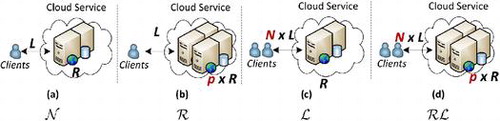
4.1. Definition of a non-scaled systems

Let’s assume that a non-scaled system (nominal system) $\mathcal{N}$ is a cloud system possessing R cloud resources and loaded with L requests, as presented in Figure 1(a)). One would expect that a non-scaled system $\mathcal{N}$ will be able to handle L amount of work in a given time period using R resources. For example, the load can be represented as the number of requests for a certain service. In this case, we assume that the service is hosted in a group of VMs using R cloud computing resources. For example, we assume a case where $L=50$ users will request a cloud service hosted on 1 VM with $R=5$ ECUs (EC2 Compute Units), which is a measure for relative processing power of an Amazon EC2 instance. Without loosing generality, we assume that each request is serial and has the same problem size. The benefit of scaling resources lies in the scaling of the number of requests, i.e. scaling the load, instead of parallelising the requests.

Figure 1. Architecture of non-scaled system $\mathcal{N}$ and possible scaled systems $\mathcal{R}$, $\mathcal{L}$ and $\mathcal{R}L$.

4.2. Definition and classification of scaled systems

We define two scaling types in cloud computing: (i) scaling the load (requirements) and (ii) scaling the cloud resources. Scaling factors for requirements and resources are usually different. Without losing generality, we assume that resources can scale up or out for $p>1$ times, while the load can increase for $N>1$ times. We will use the notation $\mathcal{L}$ or $\mathcal{R}$ to define the taxonomy of scaling the cloud systems where $\mathcal{L}$ indicates that the load is scaled, while $\mathcal{R}$ indicates that the resources are scaled.

If customers want to improve the performance of a service hosted in a cloud system, they need to scale the cloud resources. In case of scaling the load, there are two possibilities for the customer: either to retain the cost (keep the same cloud resources), which could lead to performance degradation or to scale the cloud resources and to retain the same performance, which will, however, increase their cost. Consequently, we will define three different scaled systems when only one or both parameters are scaled with Definitions 4.1–4.3. All three scaled systems are presented in Figure 1(b)–(d), correspondingly.

Definition 4.1:

[$\mathcal{R}$ scaled system] The $\mathcal{R}$ scaled cloud system denotes a cloud system with scaled Resources non-scaled Load, that is, a system that uses p times more cloud resources.

Definition 4.2:

[$\mathcal{L}$ scaled system] The $\mathcal{L}$ scaled cloud system denotes the non-scaled Resources scaled Load cloud system, that is, a cloud system with N times more load.

Definition 4.3:

[$\mathcal{R}L$ scaled system] The $\mathcal{R}L$ scaled cloud system denotes the scaled Resources scaled Load system, that is, a system that uses p times more cloud resources and N times more load.

For better presentation, we present the load and resources of the non-scaled system $\mathcal{N}$ and all three scaled systems $\mathcal{R}$, $\mathcal{L}$ and $\mathcal{R}L$ in Table 1.

Table 1. Overview of the load and resources for the non-scaled system $\mathcal{N}$ and all three scaled systems $\mathcal{R}$, $\mathcal{L}$ and $\mathcal{R}L$.

Parameter	$\mathcal{N}$	$\mathcal{R}$	$\mathcal{L}$	$\mathcal{R}L$
Load	L	L	$N·L$	$N·L$
Resources	R	$p·R$	R	$p·R$

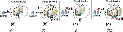
Figure 2(a) presents the three different scaling types of the non-scaled system $\mathcal{N}(R,L)$. Scaling the resources by a scaling factor p will categorise the non-scaled system $\mathcal{N}(R,L)$ to a scaled resources system $\mathcal{R}(p·R,L)$, while scaling the load to a scaled load system $\mathcal{L}(R,N·L)$. When both the resources and load are scaled, then it will categorise a system with scaled resources and scaled load $\mathcal{R}L(p·R,N·L)$. Each category of a scaled system will provide a specific performance compared to the non-scaled system.

Figure 2. Mapping a non-scaled to a scaled system.

5. A new model for efficiency of scaled systems

This section introduces the work per resource and models the speedup for scaled systems compared to a non-scaled system. Additionally, we define the efficiency specifically for each scaled system, and not only for the well-known efficiency of the system with scaled resources (the ratio of the speedup and number of processing units).

5.1. Modeling the resource utilisation

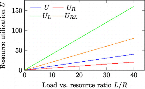
To find the resource utilisation U we determine how much average work (load) L is sent to a particular resource $R<<L$ and calculate it according to (12(12) $$\begin{array}{c}\hfill U=⌈\frac{L}{R}⌉\end{array}$$(12) ) as a ratio of the load and the number of resources. It shows the average ‘speed’ of performing a particular work per resource. In the remaining text, we will use U as abbreviation addressing the resource utilisation of the non-scaled $\mathcal{N}$ system.(12) $$\begin{array}{c}\hfill U=⌈\frac{L}{R}⌉\end{array}$$(12)

The relation for U is obtained by following a procedure to distribute all L requests in different groups, such that each group maps each of the R requests to a specific computing resource. Then, in each time period, R requests will be scattered among available R resources, which yields to (12(12) $$\begin{array}{c}\hfill U=⌈\frac{L}{R}⌉\end{array}$$(12) ). Note that the last group will have $LmodR$ requests, and not all the resources will be loaded with requests.

The resource utilisations (expressed as work per resource) $U_R$, $U_L$, $U_{\mathit{RL}}$, corresponding to the $\mathcal{R}$, $\mathcal{L}$, and $\mathcal{R}L$ systems can be presented by (13(13) $$\begin{array}{c}\hfill U_R=⌈\frac{L}{p·R}⌉;U_L=⌈\frac{N·L}{R}⌉;U_{\mathit{RL}}=⌈\frac{N·L}{p·R}⌉\end{array}$$(13) ) if the corresponding parameters are applied in (12(12) $$\begin{array}{c}\hfill U=⌈\frac{L}{R}⌉\end{array}$$(12) ).(13) $$\begin{array}{c}\hfill U_R=⌈\frac{L}{p·R}⌉;U_L=⌈\frac{N·L}{R}⌉;U_{\mathit{RL}}=⌈\frac{N·L}{p·R}⌉\end{array}$$(13)

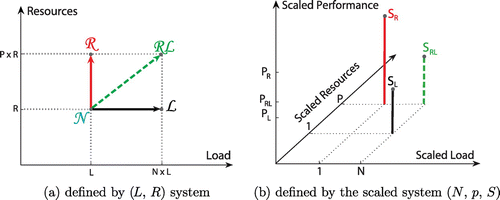
Observing the definitions for resource utilisation, one can conclude that they depend on the ratio L / R, representing a nominal value of a work per resource. We will continue with an analysis that determines the impact of the determined L / R ratio over the speedup of scaled systems. Additionally, we introduce new definitions for efficiency for each scaled system.

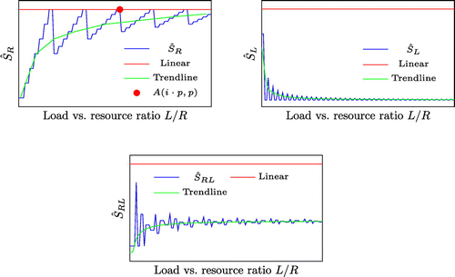
Figure 3 presents the resource utilisation of the non-Scaled system $\mathcal{N}$ and the three scaled systems $\mathcal{R}$, $\mathcal{L}$, and $\mathcal{R}L$. Observe that all resource utilisations are in a shape of stairs, with a linear trendline. The stairs’ (zig-zag) effect appears due to round up function in (12(12) $$\begin{array}{c}\hfill U=⌈\frac{L}{R}⌉\end{array}$$(12) ) and (13(13) $$\begin{array}{c}\hfill U_R=⌈\frac{L}{p·R}⌉;U_L=⌈\frac{N·L}{R}⌉;U_{\mathit{RL}}=⌈\frac{N·L}{p·R}⌉\end{array}$$(13) ). For example, if a system has four resources ($R=4$), then resource utilisation $U=3$ will be achieved for loads $L\in \{9,10,11,12\}$ because $⌈\frac{9}{4}⌉=⌈\frac{10}{4}⌉=⌈\frac{11}{4}⌉=⌈\frac{12}{4}⌉$ = 3. The next load $L=13$ will increase the resource utilisation $U=4$. We must mention that the lowest utilisation cost is achieved when R | L since the resources are fully utilised during the computation. Obviously, the resources of the $\mathcal{R}$ scaled system have a smaller amount of work, while the other two scaled systems have more, compared to the nominal system. Figure 3 is obtained for a value of $p/N=2/4=1/2$. We must note that $U_{\mathit{RL}}$ and $U_L$ can change their place in Figure 3, depending on whether the p / N ratio is greater or smaller than 1.

Figure 3. Resource utilisation of the scaled systems.

5.2. Modeling the scaled speedup limit

In order to measure the impact of scaling, (14(14) $$\begin{array}{c}\hfill {\widehat{S}}_R=\frac{U}{U_R}=\frac{⌈\frac{L}{R}⌉}{⌈\frac{L}{p·R}⌉};{\widehat{S}}_L=\frac{U}{U_L}=\frac{⌈\frac{L}{R}⌉}{⌈\frac{N·L}{R}⌉};{\widehat{S}}_{\mathit{RL}}=\frac{U}{U_{\mathit{RL}}}=\frac{⌈\frac{L}{R}⌉}{⌈\frac{N·L}{p·R}⌉}\end{array}$$(14) ) defines the limits of scaled speedup ${\widehat{S}}_R$, ${\widehat{S}}_L$, ${\widehat{S}}_{\mathit{RL}}$ for all scaled systems $\mathcal{R}$, $\mathcal{L}$ and $\mathcal{R}L$, correspondingly, when compared to the non-scaled one $\mathcal{N}$.(14) $$\begin{array}{c}\hfill {\widehat{S}}_R=\frac{U}{U_R}=\frac{⌈\frac{L}{R}⌉}{⌈\frac{L}{p·R}⌉};{\widehat{S}}_L=\frac{U}{U_L}=\frac{⌈\frac{L}{R}⌉}{⌈\frac{N·L}{R}⌉};{\widehat{S}}_{\mathit{RL}}=\frac{U}{U_{\mathit{RL}}}=\frac{⌈\frac{L}{R}⌉}{⌈\frac{N·L}{p·R}⌉}\end{array}$$(14)

We model each speedup as a ratio of resource utilisations of non-scaled system and corresponding scaled system. With the following example we briefly discuss how each equation for the maximal speedup is derived. For example, let the non-scaled system is described with $L=10$ and $R=3$, which has a resource utilisation of $U=4$ according to (12(12) $$\begin{array}{c}\hfill U=⌈\frac{L}{R}⌉\end{array}$$(12) ). Let the scaled $\mathcal{R}L$ scaled system scales the resources $p=2$ times in order to handle the scaled load of $N=3$ times, which yields to the resource utilisation of $U_{\mathit{RL}}=⌈\frac{3·10}{2·3}⌉=5$. We can observe that resource utilisation $U_{\mathit{RL}}$ is 2.5 times smaller than the resource utilisation of the non-scaled system U, which means that the scaled system’s resources are utilised 2.5 times more. This leads to the expectation that instead of achieving a speedup, the scaled system obtained a slowdown, which is expected because the load has scaled more than the resources.

Figure 4 visually presents speedups of all scaled systems as a function of the L / R ratio, along with their trend lines. The speedup limit ${\widehat{S}}_R$ shows an increasing trend starting from 1, and saturates up to the scaling factor p when $\frac{L}{R}\to \infty$. Whenever p is a divisor of L / R, the speedup limit achieves its maximal value of p, regardless of the L / R ratio value, presented by the point $A(i·p,p)$. Although it looks like that the $\mathcal{R}$ scaled system relies on the Gustafson’s Law, still it is true only when the L / R ratio is huge. For smaller L / R ratio, scaling the resources will not provide a greater speedup, which is exactly the Amdahl’s Law.

Figure 4. Speedup limits for various scaled systems as a function of L / R.

The speedup limit ${\widehat{S}}_L$ starts from ${\widehat{S}}_L=1$ and saturates its value to the point 1 / N for a greater ratio L / R. Obviously, although ${\widehat{S}}_L<p$, and seemingly it is a sublinear speedup, in fact this is a slowdown. This is expected since the load is increased compared to the non-scaled system. The resource utilisation is increased, which will reduce the performance. The trade-off for this performance suffering is the constant cost that the customer should pay for renting the resources. This is the resource underprovisioning and overutilisation.

Similar behavior for the speedup limit is presented for the $\mathcal{R}L$ scaled system. The only difference is that the trendline saturates to the value ${\widehat{S}}_{\mathit{RL}}=p/N$. Let us discuss about the expected performance of this scaled system and the calculated speedup limit (14(14) $$\begin{array}{c}\hfill {\widehat{S}}_R=\frac{U}{U_R}=\frac{⌈\frac{L}{R}⌉}{⌈\frac{L}{p·R}⌉};{\widehat{S}}_L=\frac{U}{U_L}=\frac{⌈\frac{L}{R}⌉}{⌈\frac{N·L}{R}⌉};{\widehat{S}}_{\mathit{RL}}=\frac{U}{U_{\mathit{RL}}}=\frac{⌈\frac{L}{R}⌉}{⌈\frac{N·L}{p·R}⌉}\end{array}$$(14) ). If the resource scaling follows the scaling of the work, then the speedup will saturate to 1, which means that this scaled system scales ideally. However, if $p>N$, which means overprovisioning or underutilisation, we are getting closer to the $\mathcal{R}$ scaled system, or in the hands of Amdahl’s Law.

5.3. Limiting the efficiency for each scaled system

The speedup is a standard metric used to measure the impact of scaling. Although the speedup is a common metric for the effectiveness of the scaled system, still, it does not contain any information about the efficiency, i.e. what is the achieved speedup per resource. According to our knowledge, up to now, the only metric for the efficiency is the one for the $\mathcal{R}$ scaled systems, as defined in (6(6) $$\begin{array}{c}\hfill E(n)=\frac{S(n)}{n}\end{array}$$(6) ) and (7(7) $$\begin{array}{c}\hfill E(n)=\frac{T(1)}{n·T(n)}=\frac{T(1)}{C(n)}\end{array}$$(7) ).

Since our model introduces three scaled systems ($\mathcal{R}$, $\mathcal{L}$ and $\mathcal{R}L$), we introduce (15(15) $$\begin{array}{c}\hfill {\widehat{E}}_R=\frac{{\widehat{S}}_R}{p};{\widehat{E}}_L={\widehat{S}}_L·N;{\widehat{E}}_{\mathit{RL}}={\widehat{S}}_{\mathit{RL}}·\frac{N}{p}\end{array}$$(15) ), which limits the efficiency for each corresponding scaled system, by using the speedup limits of each scaled system.(15) $$\begin{array}{c}\hfill {\widehat{E}}_R=\frac{{\widehat{S}}_R}{p};{\widehat{E}}_L={\widehat{S}}_L·N;{\widehat{E}}_{\mathit{RL}}={\widehat{S}}_{\mathit{RL}}·\frac{N}{p}\end{array}$$(15)

Let’s briefly describe how we yield the efficiency limits in (15(15) $$\begin{array}{c}\hfill {\widehat{E}}_R=\frac{{\widehat{S}}_R}{p};{\widehat{E}}_L={\widehat{S}}_L·N;{\widehat{E}}_{\mathit{RL}}={\widehat{S}}_{\mathit{RL}}·\frac{N}{p}\end{array}$$(15) ). Firstly, the ${\widehat{E}}_R$ is trivial as it is the same as the traditional efficiency according to the Amdahl’s Law. With this definition, the efficiency is limited in the range of ${\widehat{E}}_R\in (0,1]$. Exploiting this goal to limit the efficiencies of other two scaled systems $\mathcal{L}$ and $\mathcal{R}L$ to the same range (0, 1], we multiply the speedup with the load scaling factor N for scaled systems in which the load is scaled, while we divide the speedup with the resource scaling factor p for scaled systems in which the resources are scaled. Accordingly, we multiply the speedup of the $\mathcal{R}L$ scaled system with the $\frac{N}{p}$ to define the efficiency.

Although (15(15) $$\begin{array}{c}\hfill {\widehat{E}}_R=\frac{{\widehat{S}}_R}{p};{\widehat{E}}_L={\widehat{S}}_L·N;{\widehat{E}}_{\mathit{RL}}={\widehat{S}}_{\mathit{RL}}·\frac{N}{p}\end{array}$$(15) ) limits the efficiency, more important is to know the real efficiency of the scaled system, as defined in (16(16) $$\begin{array}{c}\hfill E_R=\frac{S_R}{p}=\frac{T(1)}{T_R}·\frac{1}{p};E_L=S_L·N=\frac{T(1)}{T_L}·N;E_{\mathit{RL}}=S_{\mathit{RL}}·\frac{N}{p}=\frac{T(1)}{T_{\mathit{RL}}}·\frac{N}{p}\end{array}$$(16) ), which is achieved when (5(5) $$\begin{array}{c}\hfill S(n)=\frac{V(n)}{V(1)};\mathrm{for}\mathrm{fixed}-\mathrm{time}\mathrm{algorithms}\Rightarrow S(n)=\frac{T(1)}{T(n)}\end{array}$$(5) ) is used in (15(15) $$\begin{array}{c}\hfill {\widehat{E}}_R=\frac{{\widehat{S}}_R}{p};{\widehat{E}}_L={\widehat{S}}_L·N;{\widehat{E}}_{\mathit{RL}}={\widehat{S}}_{\mathit{RL}}·\frac{N}{p}\end{array}$$(15) ) for the corresponding speedup. $T_R,T_L$ and $T_{\mathit{RL}}$ are the total execution time for each scaled system, correspondingly. Just to note that we use the fact that the cloud services are assumed as fixed-time algorithms.(16) $$\begin{array}{c}\hfill E_R=\frac{S_R}{p}=\frac{T(1)}{T_R}·\frac{1}{p};E_L=S_L·N=\frac{T(1)}{T_L}·N;E_{\mathit{RL}}=S_{\mathit{RL}}·\frac{N}{p}=\frac{T(1)}{T_{\mathit{RL}}}·\frac{N}{p}\end{array}$$(16)

The efficiency $E_R$ corresponds to already defined efficiency E(p) of the $\mathcal{R}$ scaled system. However, this metric shows the efficiency of the system with scaled resources only and it does not show the real efficiency in the case if the load is scaled. For these purposes, we introduce two more definitions for efficiencies of the other two scaled systems, in which the load is scaled, i.e. $\mathcal{L}$ and $\mathcal{R}L$.

We introduce the efficiency $E_L$ as a product of the speedup $S_L$ and the scaling factor of the load N. The following example explains some details about the efficiency $E_L$. Assume that a web server hosted in a cloud instance with one CPU core ($R=1$) can handle 50 client requests ($L=50$) with a response time of 0.5 s. The traditional approach for the efficiency E(p) yields to a wrong conclusion about the efficiency of the scaled systems $\mathcal{L}$ in the following cases: (i) doubled load $N=2$ ($L=100$) that provides response time of 1.5 s and (ii) tripled load $N=3$ ($L=150$) that provides response time of 2 s. One can calculate that (7(7) $$\begin{array}{c}\hfill E(n)=\frac{T(1)}{n·T(n)}=\frac{T(1)}{C(n)}\end{array}$$(7) ) results in an efficiency of 0.33 ($E=0.5\text{s}/(1·1.5\text{s})$) for the doubled load, while the latter will have a smaller efficiency of 0.25 ($E=0.5\text{s}/(1·2\text{s})$). Our approach results with efficiencies of $E_L=0.5\text{s}/1.5\text{s}·2=0.66$ and $E_L=0.5\text{s}/2\text{s}·3=0.75$ correspondingly, which shows that the latter scaled system is more efficient.

In order to state the problem more clearly, we present another, even more simpler example for which the classical definition of efficiency according to Amdahl’s Law is meaningless for the system with scaled resources. Let the scaled system with a single VM is loaded once with $L_1=10$ and the second time with $L_2=11$ requests. Without loosing generality, since the small load, we can assume that the response time will be the same for both loads. According to the traditional definition, the efficiency will be the same for both cases, although the latter’s resources are more utilised. How a user can exploit our model? Let’s assume that a user needs to handle 110 requests. In this case, instead of using 10 requests per VM and renting 11 VMs, the user can rent only 10 VMs and load each VM with 11 requests, still achieving the same response time and speedup.

Similarly, in the case of scaling both resources and load, the efficiency $E_{\mathit{RL}}$ of the scaled system $\mathcal{R}L$ is defined as the product of speedup $S_{\mathit{RL}}$ and the load per resources scaling factor N / p. Although this scaled system is more complex than the previous two, still the conclusions are similar that both efficiencies can be expressed by $E_L$ and $E_{\mathit{RL}}$ as a real efficiency of both scaled systems.

5.4. Going beyond the speedup limits

Although Section 5.2 presents the theoretical limits of the speedup in various scaled systems, several examples are reported where the speedup went beyond the limits, that is, a superlinear speedup is achieved.

Ristov et al. [13] have modeled the performance behavior of services classifying five sub-domains of speedup:

• Drawback: $0<S(p)<1$ - worse performance for the scaled system (a slowdown);

• No Speedup: $S(p)=1$ - the new scaled system reports the same performance as unscaled;

• Sublinear: $1<S(p)<p$ - similar to Gustafson’s scaled speedup;

• Linear: $S(p)=p$ - maximum limited speedup according to the Gustafson’s scaled speedup;

• Superlinear: $S(p)>p$ - greater performance than the limited speedup.

The expected sub-domains, along with four regions of the server load (underutilised, proportional, superior and saturated) are presented in Figure 5 [13]. The first three regions are already expressed in our theoretical analysis. In this paper the superior region is of interest, and it appears because the web server with one core will enter in its saturation mode, while the scaled system is still in its normal mode. The superior region ends when the scaled system enters the saturation mode. This means that theoretical speedups of all scaled systems do not saturate to the constant value, but they will start to falling down when the ratio L / R will increase up to some level when even the scaled resources cannot handle the load at the appropriate time.

Figure 5. Expected speedup of the $\mathcal{R}$ scaled system.

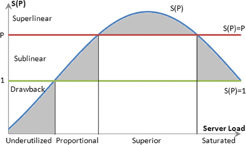
However, the reported results show that this model works only for both computation-intensive and memory-demanding web services, while the computation-intensive only web services achieve a sublinear speedup, that is, those systems have four regions.

We extend this analysis for the other two scaled systems. Table 2 models the performance of all scaled systems. We rewrite the speedup behavior for the $\mathcal{R}$ system as modeled by Ristov et al. [13].

Table 2. Modeling the sub-domains of the speedup for the three cloud scaled systems $\mathcal{R}$, $\mathcal{L}$ and $\mathcal{R}L$.

	$\mathcal{R}$	$\mathcal{L}$	$\mathcal{R}L$
Drawback	$0<S_R<1$	N/A	$0<S_{\mathit{RL}}<\frac{1}{N}$
No speedup	$S_R=1$	N/A	$S_{\mathit{RL}}=\frac{1}{N}$
Sublinear	$1<S_R<p$	$S_L<\frac{1}{N}$	$\frac{1}{N}<S_{\mathit{RL}}<\frac{p}{N}$
Linear	$S_R=p$	$S_L=\frac{1}{N}$	$S_{\mathit{RL}}=\frac{p}{N}$
Superlinear	$S_R>p$	$S_L>\frac{1}{N}$	$S_{\mathit{RL}}>\frac{p}{N}$

Let us explain the behaviors for the other two scaled systems, $\mathcal{L}$ and $\mathcal{R}L$. The drawback and No speedup behaviors do not make sense for the $\mathcal{L}$ scaled system as the resources are not scaled. The other three behaviors are determined by the load scaling factor N, or more precisely, they are determined by 1 / N. For the $\mathcal{R}L$ scaled system we observe five behavior for the speedup $S_{\mathit{RL}}$. The drawback and No speedup behaviors are determined by 1 / N, because in this case a slowdown is determined by comparing the scaled resources system and non scaled system. Other three behaviors (Sublinear, Linear and Superlinear) are determined similarly as for the $\mathcal{R}$ scaled system, and by considering the scaling load factor 1 / N, or simply they are determined by the ratio p / N.

5.5. Superlinear efficiency

Let us explain how three scaled systems can achieve superlinear efficiency defined for each system $E>1$ and what that means, similar to superlinear speedup for each scaled system. The detailed efficiency behavior is presented in Table 3. The values that determine the efficiency behavior are calculated according to Table 2 and the efficiency modeled in (15(15) $$\begin{array}{c}\hfill {\widehat{E}}_R=\frac{{\widehat{S}}_R}{p};{\widehat{E}}_L={\widehat{S}}_L·N;{\widehat{E}}_{\mathit{RL}}={\widehat{S}}_{\mathit{RL}}·\frac{N}{p}\end{array}$$(15) ) for all three scaled systems. That is, the values for the efficiency are achieved when the values of Table 2 are divided with p, 1 / N and p / N for each scaled system, correspondingly.

Table 3. Modeling the sub-domains of the efficiency for the three cloud scaled systems $\mathcal{R}$, $\mathcal{L}$ and $\mathcal{R}L$.

	$\mathcal{R}$	$\mathcal{L}$	$\mathcal{R}L$
Drawback	$0<E_R<\frac{1}{p}$	N/A	$0<E_{\mathit{RL}}<\frac{1}{p}$
No speedup	$E_R=\frac{1}{p}$	N/A	$E_{\mathit{RL}}=\frac{1}{p}$
Sublinear	$\frac{1}{p}<E_R<1$	$E_L<1$	$\frac{1}{p}<E_{\mathit{RL}}<1$
Linear	$E_R=1$	$E_L=1$	$E_{\mathit{RL}}=1$
Superlinear	$E_R>1$	$E_L>1$	$E_{\mathit{RL}}>1$

The most important observation for this modeling is the fact that all five rows of Table 3, i.e. the Drawback, No Speedup, Sublinear, Linear and Superlinear, behave the same. Our model defines all five scaled systems with the same efficiency. With this, the efficiency of different scaled systems can be compared correctly and more easily.

6. Evaluation

In this section, we present the results of a series of experiments in a cloud environment to evaluate the theoretical speedups of the scaled systems $\mathcal{R}$, $\mathcal{L}$, and $\mathcal{R}L$.

6.1. Cloud testing environment

The testing methodology and environment that are used in this paper are similar as in [14], where the authors used to determine the best scaling in Windows Azure.

We conduct all experiments in Windows Azure Cloud. The ‘PhluffyFotos’ application [15], which is a Software-as-a-Service, was deployed with different number of instances and used as a cloud elastic service. It utilises many cloud services, such as Blobs, Tables and Queues, and it interacts with the storage services of Windows Azure [16].

The application performance is measured with Apache JMeter by varying the load (the number of requests) and resources (the number of instances). The network latency is neglected because both the cloud elastic service and the client Apache Jmeter are deployed on the same data centre (West Europe’s).

The load testing is conducted by a Thread Group element, which configures the load (HTTP requests per second), one request per user. The requests simulate the concurrent accesses to a web page that displays the picture albums created by other users.

6.2. Test cases

Each test case expresses a scaled system with specific amount of resources (the number of VMs) and a specific load (number of requests per second). Each VM instance has only one CPU core and the number of VMs varies from 1 to 10.

To avoid the cloud uncertain performance [17], we repeat the execution of each test case at least 5 times and measure the average response time. The number of HTTP requests per second as a load was in the range [50, 1000], increasing the values by 50. We used this interval since the JMeter started to return error messages after 1000 requests per second.

6.3. Evaluation of the $\mathcal{R}$ scaled systems

Figure 6(a) presents the results for the speedup that five $\mathcal{R}$ scaled systems have achieved for different values of the ratio L / R, or resource utilisation. One can make three important observations:

• Scaling the system with a greater resource utilisation achieves greater speedup than scaling a system with a smaller resource utilisation.

• Scaling the system with more resources achieves greater speedup.

• Not only that the results comply with the theoretical results presented in Figure 4(a), but they go beyond the theoretical linear speedup of $S_R=p$, starting from $S{(2)}_R=2.53$ to $S{(10)}_R=18.81$. Our previous researches explain the details why and when a superlinear speedup can be achieved in a scaled system [18,19].

Although the speedup $S_R$ shows how much the scaled system $\mathcal{R}$ is better than the non-scaled $\mathcal{N}$, that is, the effectiveness of the scaling, we still cannot determine how efficient it is. The achieved efficiency $E_R$ for the same scaled system $\mathcal{R}$ is presented in Figure 6(b).

Figure 6. Performance measures of the $\mathcal{R}$ scaled system.

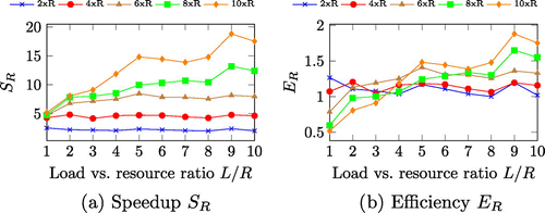
The superlinearity of the scaled systems is clearly shown when the efficiency $E_R>1$. Scaling the non-scaled system $\mathcal{N}$ with a resource utilisation $L/R\ge 4$ with any scaling factor p will provide a superlinear speedup. However, as our theoretical analysis shows, scaling the system with a great scaling factor p is inefficient when the resource utilisation L / R is low ($L/R<4$ in this case). In some cases, the scaled system can even achieve a slowdown ($S_R<1$) [13].

6.4. Evaluation of the $\mathcal{L}$ scaled systems

The speedup $S_L$ of the $\mathcal{L}$ scaled system is presented in Figure 7(a). The results again prove the theoretical analysis that scaling a non-scaled system $\mathcal{N}$ that has greater resource utilisation with the additional load will achieve less speedup than its counterpart with the lowest L / R ratio (Figure 4(b)).

Figure 7. Performance measures of the $\mathcal{L}$ scaled system.

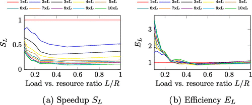
The speedup $S_L<1$ regardless of the resource utilisation L / R, for all scaled systems. The speedup $S_L$ is smaller for greater resource utilisation for the same scaled system, which proves the model by saturating to value 1 / N.

Similar to the previously observed scaled system $\mathcal{R}$, we need to analyse the efficiency of the scaled system and determine the trade-off between increasing the load and reducing the speedup. This will provide an answer which scaled system is more efficient, and for which resource utilisation L / R.

Figure 7(b) presents the efficiency $E_L$ that we have defined for the $\mathcal{L}$ scaled systems, for different starting values of the resource utilisation L / R. We observe that most efficient scaling is for the non-scaled system $\mathcal{N}$ with smaller utilisation, in our case $L/R<0.4$, since all scaled $\mathcal{L}$ systems achieved efficiency $E_L>1$. This phenomenon is a counterpart to the well-known phenomenon of the superlinear speedup in parallel scaled systems, for which the efficiency is greater of 1 since the speedup is greater of the number of processors p.

We define the phenomenon $E_L>1$ as a superlinear efficiency for the $\mathcal{L}$ scaled system, as we show in Table 3. This means that although the expected performance of the scaled system with N times more load will be reduced N times from the non-scaled system $\mathcal{N}$, still our scaled system’s performance is reduced less than N times, leading to a superlinear efficiency.

6.5. Evaluation of the $\mathcal{R}L$ scaled systems

Finally, we analyse the general case of $\mathcal{R}L$ scaled systems. Figure 8(a) presents the speedup of three different scalings (3xR, 2xL), (5xR, 3xL), and (5xR, 2xL) for various resource utilisation L / R. For simplicity and better presentation, we show only three scaled systems. The results prove the theoretical analysis that scaling a (non-scaled) system $\mathcal{N}$ both with the additional load and resources will result in a speedup towards p / N ratio (Figure 4(c)).

Figure 8. Performance measures of the $\mathcal{R}L$ system.

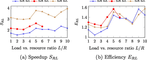
We have observed several insights for speedup of the $\mathcal{R}L$ scaled system:

• All scaled systems achieve a superlinear speedup for each resource utilisation L / R. For example, the scaled system with $p/N=1.5$ (3xR, 2xL), $p/N=1.67$ (5xR, 3xL) and $p/N=2.5$ (5xR, 2xL) achieved the maximal speedup $S_{\mathit{RL}}$ of 2.3, 2.6 and 3.95.

• The speedup curves have an ascending trend, that is, scaling a non-scaled system with a greater resource utilisation achieves greater speedup than the one with lower resource utilisation, when both systems are equally scaled.

• Despite the trend, still, there are some positive and negative peaks.

Let us explain these insights. The scaled system (5xR, 2xL) with $p/N=2.5$ has a positive peak in $L/R=5$ and $L/R=10$ in exactly those points in which the load can be most evenly distributed (scattered) to the resources, or those are the points for which p | L. The same peak in $L/R=5$ is observed for the other scaled system (5xR, 3xL). Analogue to these peaks, main peak for the scaled system (3xR, 2xL) is in $L/R=9$. Additionally, we observe smaller peaks than the extreme ($L/R=9$) again in $L/R=5$ and $L/R=10$ as they are divisors of $5·50=250$ and $10·50=500$. These observations appear since more general, $(p·R)|(N·L)$ for the scaled system, while $R\nmid L$.

Each scaled system provides a different speedup, and we analyse the efficiency $E_{\mathit{RL}}$ according to (15(15) $$\begin{array}{c}\hfill {\widehat{E}}_R=\frac{{\widehat{S}}_R}{p};{\widehat{E}}_L={\widehat{S}}_L·N;{\widehat{E}}_{\mathit{RL}}={\widehat{S}}_{\mathit{RL}}·\frac{N}{p}\end{array}$$(15) ) for the $\mathcal{R}L$ scaled system, as presented in Figure 8(b). The same peaks are observed as the efficiency $E_{\mathit{RL}}$ is proportional to the speedup $S_{\mathit{RL}}$. The comparison clearly shows which system is more efficient by comparing values of newly defined efficiency.

A superlinear speedup is achieved in each scaled system for each resource utilisation L / R. Similar to the speedup $S_{\mathit{RL}}$, the efficiency of a scaled system follows the same trend to increase for greater resource utilisation L / R.

6.6. Discussion

As the model for the efficiency behavior allows the comparison of different scaled systems, in this subsection we discuss the results for the efficiency. Similar observations can be derived, both for the speedup and the efficiency.

Table 4 shows the summary of achieved results for the efficiency for all three scaled systems. According to the results, we extract the behavior for the efficiency.

Table 4. Summary of the results for efficiency for all three cloud scaled systems.

	$\mathcal{R}$	$\mathcal{L}$	$\mathcal{R}L$
Achieved values	[0.52, 1.88]	[0.85, 3.56]	[1.04, 1.58]
Drawback	No	N/A	No
No speedup	No	N/A	No
Sublinear	Yes, $E_R\in [0.52,1)$	Yes, $E_L\in [0.85,1)$	No$\ast$
Linear	Yes	Yes	No$\ast$
Superlinear	Yes, $E_R\in [1,1.88]$	Yes, $E_L\in [1,3.56]$	Yes, $E_{\mathit{RL}}\in [1,1.58]$

We haven’t observed Drawback and No Speedup behavior for any scaled system, while other three behaviors determined by Gustafson’s Law (Sublinear, Linear and Superlinear) are observed. We have to note that for the $\mathcal{R}L$ system we observed both the Sublinear and Linear behavior for other scaled systems (e.q. $E_{\mathit{RL}}=0.96$ for (2xR, 4xL) in $L/R=3$).

Opposite to the expectation, the $\mathcal{R}$ system provided the smallest minimal efficiency of 0.52, while the $\mathcal{L}$ achieved the greatest maximal efficiency of 3.56. This insight shows the benefit of our model since it allows an easy and correct efficiency comparison of different scaled systems.

Comparing the results for the efficiency, we can conclude that the scaled systems with scaled resources, that is, $\mathcal{R}$ and $\mathcal{R}L$, improve their efficiency for greater L / R ratio, which is obvious because increasing the load to already scaled systems with resources will improve their resource utilisation. Opposite to this, the efficiency for the $\mathcal{L}$ system is maximal for smaller L / R.

We have to note that our discussion does not mean that we will have the same observation for any other system or service in cloud, but we show that with our model one can compare and determine the optimal scaling (resources or load) for a given cloud service.

7. Related work

Although the speedup of a scaled system shows the effectiveness of the scaling, still, another important parameter of the scaling is the efficiency, since it gives the information about how close are we to the ideal system. Measuring the efficiency of scaling mechanisms of different cloud providers (infrastructure as a service) and resources is an important research aspect for modeling the economics and elasticity of cloud-based applications [20].

Several researchers and standardisation organisations defined the efficiency for various parameters, such as resources, number of processors, power consumption, accuracy and completeness, operations and time. Chen et al. [7] consider the power efficiency of a cloud as a measure how the consumed power is used and define it as a performance to power ratio. The ISO/IEC 25010:2011 standard [21], on the other side, defines the efficiency from a user perspective, i.e. the amount of resources that are expended compared to the accuracy and completeness with which a user will achieve its goals. In the same standard, ISO/IEC also defines the performance efficiency as how much performance is achieved for a specific amount of resources used under stated conditions. Another approach is presented by US Defence Science Board, which considers the number of achieved compared to peak operations per second and defines this metric as computational efficiency [22]. The computation efficiency measures the execution efficiency using both the same resources and the same load. Besides the computational efficiency, Miettinen and Nurminen [23] consider the data transfer efficiency, as a measure for how much data can be transferred for a specific amount of energy, which is represented in bytes per joule. Although all these definitions are valuable since they cover many aspects of efficiency, still, none of them considers the load as we did.

Herbst et al. [6], on the other side, consider the load in the efficiency definition. They define the efficiency as how much resources are consumed in order to process some amount of work. Although they consider the load, still, they do not consider the achieved performance.

Many researchers have used the typical definition of efficiency, which is based on Amdahl’s Law, which defines the efficiency as the ratio of speedup and the number of processors. For example, Tsai et al. [24] uses the same definition, but without directly connection with the cloud elastic and heterogeneous environment. However, we present several deficiencies for the traditional efficiency definition in this paper. It assumes a homogeneous environment (6(6) $$\begin{array}{c}\hfill E(n)=\frac{S(n)}{n}\end{array}$$(6) ), which does not comply with today’s computing resources. If early clusters were homogeneous, as well as symmetric multiprocessors, most of today’s high performance computing systems are distributed and heterogeneous. In order to solve these issues, Hwang et al. [25] define the efficiency as the percentage of maximal achievable performance. They assume a heterogeneous environment and extend the definition as a ratio of the achieved speedup and the total heterogeneous cluster computing units (ECUs).

Cloud infrastructure efficiency has another challenge, besides the VMs heterogeneity. That is, due to the dynamic load and performance uncertainty, the efficiency should include both the performance and load, compared with the used resources. In this direction, Chen et al. [26] used the term scalability. They made an in-depth theoretical analysis and defined a methodology how to predict the scalability of a system/load combination. They can also predict the minimal problem size for which the scaled system will keep the scalability. However, their model uses the maximal theoretical speed versus real benchmarked speed, and cannot be used to compare two different combinations of non-scaled resource utilisation (load L and resources R) and scaled resource utilisation (load $N·L$ and resources $p·R$).

Our model with the three different definitions of efficiencies can give the answer of which scaling (scaled system) is more efficient, regardless of the scaling. Especially, our model is important for the $\mathcal{L}$ and $\mathcal{R}L$ scaled systems (scaled with load). Regardless if the efficiency is defined for the heterogeneous or homogeneous environment, one that uses the typical Amdahl’s Law-based definition will yield a wrong conclusion, as we presented an example in Section 5.3.

8. Conclusion and future work

The traditional definition of efficiency, which is based on Amdahl’s Law, shows the average speedup that is achieved when the resources are scaled up or scaled out. This definition shows the efficiency of scaling the resources, while it does not consider scaling the load and does not present system’s efficiency in this case. Another open question is the determination of the resource utilisation of both scaled and non-scaled systems.

This paper, therefore, introduces two more definitions for the efficiency, by considering the scaling of load, besides the scaling of resources. That is, we develop and classify three types of scaled systems, (i) scaled resources only, (ii) scaled load only, and (iii) scaled both the resources and load. Our model describes the general scaling in cloud analysing both the load and resources. With this, we can determine how efficient will be the scaled system, compared to the non-scaled, including all relevant factors about current and scaled load and resources. The most important contribution is presented in Table 3, which shows that the values for efficiency for each scaled system are the same for each sub-domain (Drawback, No Speedup, Sublinear, Linear and Superlinear).

We introduce the superlinearity of the scaled system with N times more load, where the scaled system’s performance are reduced less than N times of the non-scaled system. Our new definitions of the efficiency help to observe immediately the superlinearity, as well as to compare which scaled system is more efficient for constant resource utilisation. The gained conclusions can be generalised since all theoretical analyses are proven by the series of experiments conducted in Windows Azure Cloud.

Using the model, one can define the load balancing and auto scaling policies in the cloud. We can avoid the load – resource combinations that comply with Amdahl’s Law, and use only those combinations that follow the Gustafson’s Law and especially address the superlinear regions. In this case, end point servers that host the elastic cloud services will be utilised at maximal efficiency.

Our future work will be to develop such load balancing and auto scaling policies based on these models of speedups and efficiencies, which will be more efficient than the current state of the art. Since various VM types consist of different amount of virtual CPUs, RAM memory, storage size and networking, we will extend this research towards splitting resource types as computing (CPU), memory capacity and storage in order to define more detailed CPU, memory, storage and network elasticity models. Additionally, we will extend the task types by introducing dependencies, i.e. to use scientific and business workflows.

Disclosure statement

No potential conflict of interest was reported by the authors.

Additional information

Funding

This work is being accomplished as a part of (i) ENTICE: dEcentralised repositories for traNsparent and efficienT vIrtual maChine opErations, funded by the European Unions Horizon 2020 research and innovation programme [grant agreement number 644179], and (ii) Tiroler Cloud: Energiebewusste Föderierte Cloud für Anwendungen aus Industrie und Forschung, funded by the Österreichische Forschungsförderungsgesellschaft [grant agreement number 848448].

References

- Armbrust M, Fox A, Griffith R, et al. A view of cloud computing. Commun ACM. 2010;53:50–58.
- Gupta A, Milojicic D. Evaluation of HPC applications on cloud. In: Open cirrus summit (OCS). Atlanta, GA; 2011 Oct. p. 22–26.
- Tsaftaris SA. A scientist’s guide to cloud computing. Comput Sci Eng. 2014;16:70–76.
- Liu L, Zhang M, Lin Y, et al. A survey on workflow management and scheduling in cloud computing. In: 14th IEEE/ACM International Symposium on Cluster, Cloud and Grid Computing (CCGrid). Chicago, IL; 2014 May. p. 837–846.
- Evans E, Grossman R. Cyber security and reliability in a digital cloud. Washington (DC): US Department of Defense Science Board Study; 2013.
- Herbst NR, Kounev S, Reussner R. Elasticity in cloud computing: what it is, and what it is not. In: Proceedings of the 10th International Conference on Autonomic Computing (ICAC 13); San Jose, CA: USENIX:2013. p. 23–27.
- Chen Q, Grosso P, van der Veldt K, et al. Profiling energy consumption of VMs for green cloud computing. In: 2011 IEEE Ninth International Conference on Dependable, Autonomic and Secure Computing. Sydney, NSW, Australia; 2011 Dec. p. 768–775.
- Amdahl GM. Validity of the single-processor approach to achieving large scale computing capabilities. In: AFIPS Conference Proceedings; Apr 18--20; Reston. VA. Vol. 30; Atlantic City, NJ: AFIPS Press; 1967. p. 483–485.
- Ristov S, Prodan R, Gusev M, et al. Elastic cloud services compliance with Gustafson’s and Amdahl’s laws. In: Third International Workshop on Sustainable Ultrascale Computing Systems (NESUS 2016); 2016 Dec. p. 1–9. Available from: http://e-archivo.uc3m.es/handle/10016/24223
- Gustafson JL. Reevaluating Amdahl’s law. Commun ACM. 1988;31:532–533.
- Gustafson J, Montry G, Benner R. Development of parallel methods for a 1024-processor hypercube. SIAM J Sci Stat Comput. 1988;9:532–533.
- Lehrig S, Eikerling H, Becker S. Scalability, elasticity, and efficiency in cloud computing: a systematic literature review of definitions and metrics. In: International ACM SIGSOFT Conference on Quality of Software Architectures, QoSA ’15. Montreal: ACM; 2015. p. 83–92.
- Ristov S, Gusev M, Velkoski G. Modeling the speedup for scalable web services. In: Bogdanova AM, Gjorgjevikj D, editors. ICT Innovations 2014. Vol. 311, Advances in intelligent systems and computing. Springer International Publishing; 2015. p. 177–186. Available from: http://link.springer.com/chapter/10.1007/978-3-319-09879-1_18
- Gusev M, Ristov S, Koteska B, et al. Windows Azure: resource organization performance analysis. In: Villari M, Zimmermann W, Lau KK, editors. Service-oriented and cloud computing (ESOCC). Vol. 8745, LNCS. Berlin Heidelberg: Springer; 2014. p. 17–31.
- Microsoft, Picture gallery service; 2012 [cited 2017 Sep 9]. Available from: http://phluffyfotos.codeplex.com/
- Zhang L, Ma X, Lu J, et al. Environmental modeling for automated cloud application testing. Softw IEEE. 2012;29:30–35.
- Math R, Ristov S, Prodan R. Simulation of a workflow execution as a real cloud by adding noise. Simul Model Pract Theory. 79:37–53. Available from: http://www.sciencedirect.com/science/article/pii/S1569190X17301351
- Gusev M, Ristov S. A superlinear speedup region for matrix multiplication. Concurrency Comput: Pract Exp. 2013;26:1847–1868. DOI:10.1002/cpe.3102
- Ristov S, Prodan R, Gusev M, et al. Superlinear speedup in HPC systems: why and when? In: 2016 Federated Conference on Computer Science and Information Systems (FedCSIS); Gdansk, Poland: IEEE; 2016 Sept. p. 889–898. Available from: http://ieeexplore.ieee.org/document/7733347/
- Suleiman B, Sakr S, Jeffery R, et al. On understanding the economics and elasticity challenges of deploying business applications on public cloud infrastructure. J Internet Serv Appl. 2012;3:173–193. DOI:10.1007/s13174-011-0050-y
- ISO/IEC. ISO/IEC 25010 – systems and software engineering – systems and software quality requirements and evaluation (SQuaRE) – system and software quality models (2010) by ISO/IEC. Technical report; 2010. Available from: https://www.iso.org/standard/35733.html
- US Defense Science Board, Cyber security and reliability in a digital cloud. US Department of Defense Science Board Study; 2013. Available from: http://www.dtic.mil/dtic/tr/fulltext/u2/a581218.pdf
- Miettinen AP, Nurminen JK. Energy efficiency of mobile clients in cloud computing. In: Proceedings of the 2Nd USENIX Conference on Hot Topics in Cloud Computing, HotCloud’10; Boston, MA: USENIX Association; 2010. p. 4–4. Available from: http://dl.acm.org/citation.cfm?id=1863103.1863107
- Tsai WT, Huang Y, Shao Q. Testing the scalability of SaaS applications. In: Proceedings of the 2011 IEEE International Conference on Service-Oriented Computing and Applications, SOCA ’11. Irvine (CA): IEEE Computer Society; 2011. p. 1–4. DOI:10.1109/SOCA.2011.6166245
- Hwang K, Bai X, Shi Y, et al. Cloud performance modeling with benchmark evaluation of elastic scaling strategies. IEEE Trans Parallel Distrib Syst. 2016;27:130–143.
- Chen Y, Sun XH, Wu M. Algorithm-system scalability of heterogeneous computing. J Parallel Distrib Comput. 2008;68:1403–1412.