Precision in estimates of density and biomass of Norwegian spring-spawning herring based on acoustic surveys

Abstract

The abundance and biomass of the Norwegian spring-spawning herring (NSSH) stock are assessed annually using a virtual population analysis (VPA) applied to catch-at-age data from the fishery and fishery-independent abundance indices derived from research vessel surveys for calibration (‘tuning’). The most important of these surveys is the International Ecosystem Survey in the Nordic Seas (IESNS) and this is highly influential for the outcome of the assessment. Until now, the abundance indices from the IESNS have been reported without any measure of uncertainty. In this study, the sampling errors associated with the density estimates of NSSH from the IESNS for the years 2009–2012 are estimated using design-based survey sampling theory. The annual survey estimates of number and biomass of herring per square nautical mile (nm²) were relatively precise for all age groups combined, with relative standard error (RSE) ranging from 8% to 15%, while for each individual age group (3–12) the RSE was less than 30% for most years. For age groups 1 and 2, and all age groups older than 12 years, the density estimates are highly imprecise, with RSE ranging from 30% to 100%. The precision in estimated density provided here indicates that the time series from the survey can be used to study trends in overall abundance and biomass of the stock. It is recommended that statistical assessment models that can account for sampling errors in input data from survey indices by age group and catch-at-age be tested in the assessments of the NSSH stock.

Key words:

• Abundance estimate
• acoustic transect survey
• herring
• precision
• stock assessment

Introduction

Norwegian spring-spawning herring (NSSH) is the largest herring (Clupea harengus Linnaeus, 1758) stock in the world, and supports a highly valuable commercial fishery with quotas that are shared among the coastal states of Norway, Iceland, Russia, Faroe Islands and the EU. The spawning stock biomass (SSB) has fluctuated greatly over time, with a maximum of 16 million tons estimated for 1945, while the most recent estimate was 5 million tons (ICES 2013a). NSSH is a highly migratory stock that spawns along the Norwegian coast, has its main nursery areas in the Barents Sea and its main feeding areas in the Norwegian Sea. NSSH has major roles in these ecosystems, both as a consumer of zooplankton and as a source of prey for larger predators (Holst et al. 2004). The International Council for the Exploration of the Sea (ICES) conducts annual assessments of the NSSH stock, using virtual population analysis (VPA; e.g. Shepherd 1999) to estimate fishing mortality (F) and SSB. Several acoustic survey indices of abundance are used as tuning series for calibration in the VPA (ICES 2013a). The yearly survey indices of abundance are currently reported without any measures of precision and hence it is difficult to quantify the total uncertainty of the stock assessment results. The most important tuning series used for calibration in the assessment is based on the ICES-coordinated International Ecosystem Survey in the Nordic Seas (IESNS), which has been conducted annually during May by the coastal states since 1995. In the beginning of the feeding season in May, NSSH is distributed in the Nordic Seas from around 62°N to 75°N and from 15°W to the Norwegian coast and into the Barents Sea (Figure 1). The IESNS is the only survey that covers the spatial distribution of the entire stock and it produces the only age-disaggregated abundance indices used as tuning series, which is updated annually, in the assessment. Indices of abundance based on the IESNS has relatively high correlation between cohorts from consecutive years (internal consistency), indicating that it is possible to track a year-class of herring over time based on this survey (ICES 2013a). Accordingly, since 1995 this survey has had a high influence on the assessment and the advice on total allowable catch (TAC). As a result, the cohort estimates of abundance from the survey closely tracks the annual age-based assessments of stock size, particularly for the big year-classes. Because of its high influence on the assessment it is particularly important to provide precision estimates of the abundance indices from this survey.

Figure 1. Map of the study area for the ICES-coordinated International Ecosystem Survey in the Nordic Seas (IESNS) in May–June.

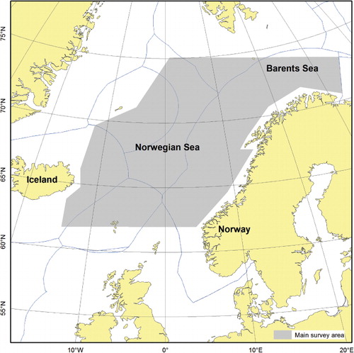
The IESNS is conducted at the beginning of the summer feeding season for NSSH and in some years a component of the stock was still actively migrating towards the feeding grounds during this period, requiring synoptic survey coverage to minimize the potential effects of migration. The herring stock has exhibited shifts in behaviour over the years since the initiation of the survey in 1995, and can be found either in small, loosely packed schools in the upper 50 m, or in dense schools of varying size near the surface, in intermediate (50–200 m) or in deeper waters (200–400 m). The horizontal distribution of the stock during May has also varied. Generally, the distance of the feeding migration and the horizontal distribution of the stock increased with the increasing stock size during the first half of the period, but has been more stable thereafter (ICES 2013a). Thus, since 2009 the adult stock has occupied most of the survey area of around 800,000 km² in the Norwegian Sea and adjacent waters (Figure 1). Clearly, the changes in spatial distributions over time, both horizontally and vertically, may introduce biases in acoustic indices of abundance of changing magnitudes and directions. Such biases can be caused by vessel avoidance, acoustic shadowing and depth-dependent acoustic target strength (Skaret et al. 2005; Løland et al. 2007; Hjelvik et al. 2008). For other species authors have focused on varying catchability related to bottom trawl surveys (Thorson et al. 2013), acoustic deadzones near the bottom (Ona & Mitson 1996), or the use of combined acoustic and bottom trawl data to improve abundance estimates (Godø & Wespestad 1993; McQuinn et al. 2005; Kotwicki et al. 2012). We acknowledge that the effect of varying catchability is also relevant for herring in the present survey. However, we focus on the precision of annual survey indices from the IESNS, which is determined primarily by the spatial distribution (patchiness) of the stock, survey design and sampling effort (sample sizes in terms of the number of acoustic transects within strata). Random sampling errors in acoustic survey indices of abundance due to spatial sampling have been shown to be the main source of uncertainty in acoustic measurements of abundance (Rose et al. 2000). Løland et al. (2007) investigated a number of additional sources of error in acoustic survey estimates of the NSSH stock in the wintering area. They did, however, conclude that acoustic sampling error (variation among transects) was the largest contributor to the total uncertainty of the estimate.

A quantitative understanding of the precision of survey abundance indices is an advantage for assessment and fishery management. Uncertainty in stock assessments based on VPA is related to precision and bias in input data on catch-at-age data from fisheries-dependent surveys and abundance indices from fisheries-independent surveys. The sampling errors associated with the estimates from the IESNS have not been estimated thoroughly or presented previously. The main objective here is to contribute to uncertainty estimates in the future assessments of the stock. Statistical assessment models provide a possible framework for assessing the effects of uncertainty related to precision and bias in input data (Nielsen & Berg 2014).

Material and methods

The combined acoustic and trawl survey

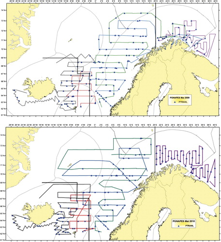
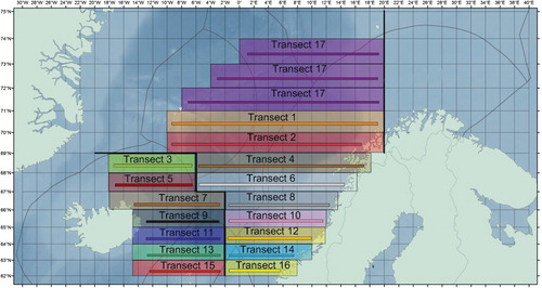
IESNS follows a stratified systematic transect design, where three subareas (strata) are covered by systematic acoustic transects with varying degrees of overlap between the vessels from the different participating nations (Figure 2). The acoustic transects are evenly spaced to minimize the effects of local positive autocorrelation and thereby maximize the precision in abundance and biomass estimates (Simmonds & Fryer 1996; Harbitz & Aschan 2003; Simmonds & MacLennan 2005; Walline 2007). The area covered by the survey has been confined within the latitude–longitudes around 34°E–14°W and 62–74°N since 1995, with some variation due to variation in the distribution of the NSSH stock. In this work we focus only on the two strata in the Norwegian Sea because the abundance indices used in the assessment are based on data from these strata only, i.e. the adult stock. Integrated acoustic data are recorded continuously along the cruise tracks, and scrutinized and stored at a resolution of 1 nautical mile (nm). The acoustic transects form the primary sampling units (PSUs); transects that crossed strata boundaries were split and treated as independent units (Figure 3). Trawl samples are collected along the cruise track to estimate the composition of fish communities by species, length, weight and age. The acoustic density estimates are converted to age-disaggregated biomass estimates based on the length, weight and age distributions from the targeted trawl samples. The method used to calculate the precision of the density estimates is described below. We calculated the relative standard error (RSE) to evaluate the precision of the IESNS abundance and biomass indices for the years 2009–2013. The reason for the analysis being restricted to this five-year period was that it was time-consuming to extract the data necessary for the analysis and it was decided that five years of data were enough for the present purpose. RSE is defined as the proportion of the sampling standard error to the estimate of a population characteristic (Jessen 1978).

Figure 2. Cruise tracks for the ICES-coordinated International Ecosystem Survey in the Nordic Seas (IESNS) in 2009 and 2010. Cruise tracks of the five vessels are shown in separate colours.

Figure 3. Transects used in the estimation of mean density and biomass with associated variance. Thick lines indicate the borders between the three strata, two strata in the Norwegian Sea and one in the Barents Sea. The strata in the Barents Sea (east of transect 17) does not include any transects, as these are not used in the present article.

Acoustic methods for estimating density of herring within transects

Acoustic recordings of fish and plankton are collected continuously during the survey and integrated using calibrated ER60 echosounder systems with a primary operating frequency of 38 kHz. Post-processing software differs among the vessels and years, but all participants use the same post-processing procedure, last verified and agreed upon at a scrutinizing workshop in Bergen in February 2009 (ICES 2009). To estimate the abundance, the allocated s_A-values (acoustic area backscattering coefficients; MacLennan et al. 2002) are averaged for geographical rectangles (1° latitude × 2° longitude) within each stratum, h (Figure 3). Biological samples from trawl catches along transects are used to partition the echo backscattering by species and to convert echo-integration data to biomass. The trawling is conducted primarily in areas with strong echo signals attributed to NSSH. For geographic rectangles without trawl catches, biological samples from trawl stations in neighbouring rectangles are chosen manually by experts to represent the species composition. The GIS-based BEAM software (Totland & Godø 2001) was used to optimize the allocation of biological samples from trawl stations to the hydroacoustic data to produce the estimates of total biomass and numbers of individuals by age and length for the statistical rectangles j that overlap each transect. For each statistical rectangle j in stratum h and transect i, the unit area density of fish in number per square nautical mile () is calculated using standard equations (Foote et al. 1987; Toresen et al. 1998). The target strength (TS) for herring is the one used traditionally, TS = 20.0 log₁₀(L) – 71.9 dB (Foote et al. 1987). The density of herring in number of fish per nm² for each primary sampling unit (transect; Figure 3) is then simply taken as the mean of the density estimates for the statistical rectangle j that overlap each transect. The biomass density (tons per nm²) for each transect is estimated by multiplying density in numbers by the average weight of the fish for each transect. The angle of the acoustic beam is approximately 7° for all vessels, and the diameter of the acoustic beam is 24.5 m at 200 m depth and 36.7 m at 300 m depth. Thus, the actual area covered by each transect is only a negligible fraction of the total area of the statistical rectangles along each transect. Hence, we use the transect length as a measure of cluster size, and not the sum of the areas for the j statistical rectangles that overlap each transect. Total abundance or biomass of the entire survey area is simply obtained by expanding the mean density to the total area. In the following, we present estimators of mean density and associated precision for the NSSH based on the IESNS.

Estimators of mean density of herring and associated variance

To estimate the mean density of herring (number or biomass per nm²) in the total survey area along with the associated precision, we follow a similar approach as Jolly & Hampton (1990), treating the acoustic transect survey as a stratified cluster sampling design, with primary sampling units (transects) of unequal size (e.g. Cochran 1977; Wolter 1985; Lehtonen & Pahkinen 2004) due to the variable transect lengths. We follow Jolly & Hampton (1990) and assume that the n_h primary sampling units (transects) were selected as a simple random sample from all possible transects within each stratum h. The approximate variance estimator which regards a systematic sample as a simple random sample is common (e.g. Wolter 1985: 250). We applied a separate ratio estimator (Cochran 1977; Jolly & Hampton 1990) to estimate the overall mean density across strata and the associated sampling errors. An estimator for the mean density within stratum h is

(1)

and a Taylor approximation for the variance of Equation (1) under the assumption of simple random sampling of transects within strata (Cochran 1977) is given as

(2)

where denotes the estimated mean density of herring within transect i in stratum h, l_hi denotes the transect lengths, is the mean transect length, and n_h is the number of transects in stratum h. The transect length l_hi is a random variable under random sampling of transects. The among-transect variation of mean density, as well as the variation in cluster sizes (transect lengths), contributes to the variance of Equation (1). Because the denominator in the ratio estimator of Equation (1) is a random variable, an exact analytical variance estimator is not available (Cochran 1977: 303–304). Therefore, we use bootstrap to estimate the variance of Equation (1) in addition to the linearization method, Equation (2). The bootstrap estimation of variance within each stratum introduces a bias of (n_h – 1)/n_h (see e.g. Korn & Graubard 1998; Lehtonen & Pahkinen 2004). This bias can be substantial when sample size n_h is low within a stratum, which is the case for the IESNS, and we therefore rescaled each bootstrap estimate of the variance by n_h/(n_h – 1) (Lehtonen & Pahkinen 2004: 160–161).

We have assumed fixed acoustic transect widths in the estimation of mean densities, and hence use transect length as a measure of cluster size. Because the transect width is narrow compared to the size of the survey area, the number of transects sampled in each stratum is insignificant as compared to the total number of possible transects. Hence, the sampling fraction is approximately zero. We therefore used Equation (2), and also bootstrapping with replacement (Efron 1982) from the primary samples (transects), to estimate the variance of Equation (1) (Williams 2000). An estimator for the overall mean density across strata is then simply obtained by combining the ratio estimates using strata weights,

(3)

with the variance of Equation (2) estimated by the usual stratified estimator

(4)

with strata weights

(5)

The precision of the estimated overall mean density is given by . The estimates of density and associated RSE by year-class were obtained using the R survey library (Lumley 2010).

Results

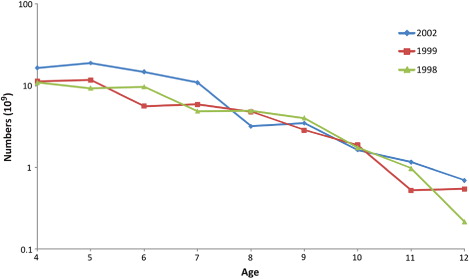
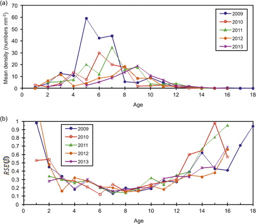
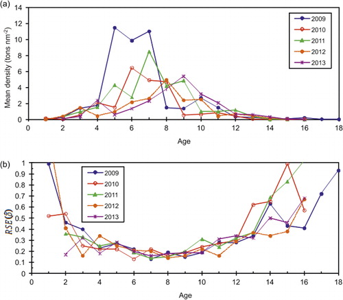
The estimated annual abundance in numbers-at-age from the IESNS seems to track the strong year-classes relatively well over time. As an example, we show abundance estimates for the strong 1998, 1999 and 2002 year-classes from several successive surveys (Figure 4). The figure shows a generally declining trend in the size of the cohorts, indicating that cohorts are followed reasonably well in the survey. The RSE in estimated density for herring in all age groups combined ranged from 8% to 15% (Tables I, II). The density in numbers or biomass per nm² for age groups 3–12 had RSE of less than 30% for most years (Tables I, II; Figures 5, 6). For age groups 1–2, and ages above 12, the density estimates were highly imprecise, with RSE ranging from 30% to 100%. Estimates of the mean density in the survey area ranged from a maximum of 201 × 10³ herring per nm² in 2009 (RSE = 15%) to a minimum of 19 × 10³ herring per nm² (RSE = 13%) in 2012 (Figure 7). In the recent period, the survey indices from the years 2010 and 2012 deviated most from the ICES assessment, and also had relatively low RSE, indicating that there are additional sources of uncertainty not accounted for here.

Table I. Stratified mean density (thousands per nm²), standard error (SE) and relative standard error (RSE) in numbers at age from 2009 to 2013 based on IESNS using the ratio estimator within strata. The standard error is estimated based on bootstrapping with 5000 replicates within each stratum.

	2009			2010			2011			2012			2013
Age
1	0.84	0.82	0.98	3.08	1.64	0.53	0	0		0.03	0.04	1.24	0	0
2	4.29	1.94	0.45	1.3	0.71	0.54	5.12	1.74	0.34	6.29	2.99	0.48	1.59	0.45	0.28
3	12.83	4.42	0.34	4.1	1.22	0.3	5.72	1.74	0.3	11.61	1.83	0.16	2.88	0.91	0.32
4	10.79	1.98	0.18	13.41	3.78	0.28	7.28	1.89	0.26	1.93	0.62	0.32	12.05	2.24	0.19
5	59.2	16.29	0.28	7.44	1.54	0.21	20.21	5.85	0.29	4.23	1.19	0.28	2.53	0.75	0.3
6	42.3	8.81	0.21	29.9	3.62	0.12	11.99	2.44	0.2	8.68	1.86	0.21	5.22	1.07	0.21
7	44.17	5.7	0.13	20.19	4.78	0.24	34.64	5.06	0.15	9.99	2.01	0.2	8.7	1.4	0.16
8	5.62	1.14	0.2	17.82	2.91	0.16	15.9	2.27	0.14	18.54	2.74	0.15	13.61	2.43	0.18
9	4.84	0.77	0.16	1.89	0.38	0.2	17.85	3.47	0.19	8.42	1.32	0.16	18.97	3.76	0.2
10	9.14	1.69	0.19	2.14	0.52	0.24	3.52	1.11	0.32	8.57	1.86	0.22	10.82	2.18	0.2
11	4.89	1.36	0.28	2.81	0.77	0.27	3.41	0.81	0.24	1.36	0.24	0.18	6.99	2.19	0.31
12	1.07	0.29	0.27	1.34	0.41	0.3	4.07	1.41	0.35	2.2	0.61	0.28	2.05	0.69	0.34
13	0.95	0.37	0.39	0.12	0.07	0.6	1.17	0.45	0.39	1.34	0.47	0.35	1.82	0.61	0.33
14	0.27	0.17	0.62	0.1	0.06	0.65	0.05	0.03	0.67	0.4	0.13	0.33	0.78	0.35	0.44
15	0.24	0.1	0.43	0.01	0.01	0.98	0.06	0.05	0.81	0.05	0.02	0.38	0.16	0.07	0.45
16	0.53	0.22	0.41	0.09	0.05	0.57	0.03	0.03	0.95	0.13	0.08	0.66	0.03	0.02	0.69
17	0.07	0.05	0.71	0	0		0	0		0	0		0	0
18	0.03	0.03	0.94	0	0		0	0		0	0		0	0
Tot	202.07	30.75	0.15	105.74	8.36	0.08	131.01	17.95	0.14	83.78	10.68	0.13	88.21	12.1	0.14

Table II. Stratified mean density (tons nm⁻²), standard error (SE) and relative standard error (RSE) in biomass at age from 2009 to 2013 based on IESNS using the ratio estimator within strata. The standard error is estimated based on bootstrapping with 5000 replicates within each stratum.

	2009			2010			2011			2012			2013
Age
1	0.01	0.01	0.99	0.13	0.07	0.52	0	0		0	0	1.26	0	0
2	0.24	0.11	0.46	0.05	0.03	0.54	0.29	0.1	0.36	0.36	0.15	0.41	0.08	0.01	0.17
3	1.4	0.56	0.4	0.55	0.14	0.25	0.96	0.32	0.33	1.47	0.23	0.16	0.35	0.11	0.32
4	1.73	0.4	0.23	2.1	0.46	0.22	1.52	0.39	0.25	0.41	0.14	0.34	2.35	0.42	0.18
5	11.49	3.15	0.27	1.48	0.32	0.22	4.27	1.19	0.28	0.96	0.24	0.25	0.59	0.16	0.28
6	9.81	2.14	0.22	6.42	0.81	0.13	2.77	0.53	0.19	2.15	0.45	0.21	1.34	0.27	0.2
7	10.96	1.4	0.13	4.9	1.1	0.22	8.44	1.19	0.14	2.6	0.51	0.2	2.31	0.36	0.16
8	1.48	0.29	0.19	4.72	0.77	0.16	4.19	0.63	0.15	4.92	0.71	0.14	3.76	0.67	0.18
9	1.35	0.2	0.15	0.53	0.1	0.19	4.84	0.95	0.2	2.37	0.37	0.16	5.39	1.05	0.19
10	2.67	0.5	0.19	0.63	0.15	0.24	0.99	0.3	0.31	2.46	0.55	0.22	3.16	0.61	0.19
11	1.46	0.41	0.28	0.83	0.23	0.27	1	0.24	0.24	0.41	0.07	0.16	2.07	0.65	0.31
12	0.33	0.09	0.28	0.41	0.12	0.3	1.17	0.38	0.32	0.67	0.19	0.29	0.63	0.21	0.34
13	0.27	0.09	0.34	0.04	0.02	0.62	0.35	0.13	0.37	0.41	0.15	0.37	0.58	0.19	0.32
14	0.09	0.06	0.63	0.03	0.02	0.65	0.02	0.01	0.69	0.12	0.04	0.34	0.29	0.14	0.5
15	0.09	0.04	0.43	0	0	0.99	0.02	0.02	0.83	0.02	0.01	0.38	0.05	0.02	0.46
16	0.18	0.07	0.41	0.03	0.02	0.57	0.01	0.01	1.02	0.04	0.03	0.67	0.01	0.01	0.68
17	0.03	0.02	0.72	0	0		0	0		0	0		0	0
18	0.01	0.01	0.93	0	0		0	0		0	0		0	0
Tot	43.63	6.41	0.15	22.84	2.03	0.09	31.04	4	0.13	19.32	2.61	0.14	22.97	3.23	0.14

Figure 4. Estimated numbers at age from the IESNS for the 1998, 1999 and 2002 year-classes. Numbers are corrected by estimated survey catchability-at-age and are plotted on a logarithmic scale.

Figure 5. Mean density of abundance (thousands per nm²) per age group as obtained from the IESNS (a) along with associated precision (b).

Figure 6. Mean density of biomass (tons per nm²) per age group as obtained from the IESNS (a) along with associated precision (b).

Figure 7. Spawning stock biomass (SSB) from the assessment is shown by the blue line while the estimate from the IESNS is shown by the red line, with approximate 95% confidence intervals for the years 2009–2013.

Discussion

We treated the IESNS design as if simple random samples of transects were selected within strata in the analysis in order to obtain design-based estimates (Cochran 1977) of precision. This was also done by Jolly & Hampton (1990). The true precision is likely to be higher than we estimated because the systematic and even spacing of transects minimizes the spatial correlation among neighbouring observations (Cochran 1977). The RSE estimates based on the Taylor linearization method (Equation (2)) were nearly identical but slightly lower (i.e. higher precision) than for the bootstrap method. However, it is well known that the linearization method can yield variance estimates that are biased downwards when sample sizes are low (e.g. Cochran 1977: 304). We only present results from the bootstrap method here.

We ignored the acoustic registrations obtained along the ship track between the systematically spaced transects in this study. These data could be used in a model-based estimation of densities and associated precision. The reason for not using geostatistical methods to estimate precision (Walline 2007) is that the acoustic transects in the IESNS were spaced so far apart (60 nm) that the local autocorrelation across transects is negligible. The only continuous recording of acoustic data across transects is from the ship track that connects transects at the edges of the survey area. Variograms estimated from continuous acoustic recording along transects, or from acoustic recordings along the ship track that connect transects, may not be representative in all directions of the survey area.

In contrast to the standard method for estimating acoustic survey indices for NSSH, which is based on averaging of estimates by geographical rectangles (1° latitude × 2° longitude), we treated the acoustic transects as primary sampling units (PSUs). The bootstrap of transects should provide more realistic estimates of precision than methods where the geographical rectangles or segments of transects are treated as PSUs and assumed to be independent. Uncertainty around the yearly trawl-acoustic estimate of biomass of Barents Sea capelin (Tjelmeland 2002), for example, is routinely quantified based on resampling of acoustic integrator values in rectangles. However, integrator values in rectangles spaced closely together may be correlated. Because of the 1° (60 nm) spacing between transects in the north–south direction in the IESNS, it is reasonable to assume independence between transects. For North Sea herring, for example, it has been observed that the schools may be linked with oceanographic features on scales of 5–20 km (~3–11 nm), giving some medium-scale spatial correlation (Maravallias et al. 1996). Simmonds et al. (2009) observed that with an average transect spacing of 15 nautical miles (approximately 24 km), little could be inferred from one transect to the next for Peruvian anchoveta. When the sampling fraction of PSUs is negligible as for the IESNS analysed here, it can be reasonably assumed that the PSUs are sampled with replacement and there is therefore no need to estimate the variance of density estimates within PSUs (transects) (Williams 2000). Hence, the autocorrelation of density at finer scales along transects can be ignored when estimating the RSE of the overall density across strata.

Several additional factors could contribute to uncertainty in our estimates. We assumed that all transect samples were independent between strata, while in actuality many of the acoustic transects in the Norwegian Sea crossed strata. A truly stratified survey could be achieved by selecting transects independently within strata (this was done for the 2014 IESNS). Also, following Jolly & Hampton (1990), we did not attempt to quantify systematic errors (bias) due to factors such as the acoustic scrutinizing process, calibration constants and vessel effects, etc. Factors such as vessel avoidance, acoustic shadowing and depth-dependent acoustic target strength can cause systematic errors (bias) that are not accounted for in this article (Skaret et al. 2005; Løland et al. 2007; Hjelvik et al. 2008). However, the effect of depth-varying acoustic target strength is being investigated in a separate study. A number of authors have focused on acoustic deadzones near the bottom (Godø & Wespestad 1993; Ona & Mitson 1996; McQuinn et al. 2005; Kotwicki et al. 2012). The IESNS is a pelagic survey conducted in a deep ocean, but an acoustic deadzone near the surface might be a source of bias. Work is underway using a combination of sonar and echo sounder to investigate this effect. However, it should be noted that random errors due to spatial variation in herring abundance and species composition of fish, as well as random variations in the relationships between target strength and length of herring, will be partly reflected in the sampling errors (see Jolly & Hampton 1990).

The current sampling effort in the IESNS produces relatively precise overall estimates of density and biomass of the stock for the years 2009–2013, with RSE ranging from 8% to 15%. The estimates satisfy Level 1 precision requirements specified by the European Commission (EC) for many survey estimates used for management in the fisheries sector in the EU for the period 2011–2013 (Anon 2010). The EU Level 1 precision requirement specifies that it should be possible to estimate a parameter within plus or minus 40% for a 95% confidence level and an RSE of 20% for the parameter estimate is used as an approximation. Level 1 is the least strict precision requirement. Levels 2 and 3 require RSEs of 12.5% and 2.5%, respectively. No minimum precision requirements are established for abundance surveys in ICES. Because of the commercial value of the NSSH fishery, survey estimates of abundance with at least Level 2 precision would be desirable, and could be achieved without prohibitive costs. Precise estimates of abundance indices are essential for responsible stewardship of marine resources and the US National Oceanic and Atmospheric Administration (NOAA) and National Marine Fisheries require that precision estimates be provided for abundance estimates of major pelagic and groundfish stocks based on trawl and acoustic surveys.

The IESNS estimates of density and biomass for individual age groups from 3 to 12 are less precise than for all age groups combined, but the RSEs are generally less than 30%. For ages younger and older than this, the estimated density is highly imprecise (RSE > 30%) and such a pattern of imprecise estimates at extreme ages is also found in surveys for other herring stocks (Woillez et al. 2009). Age groups that occupy a relatively small portion of the survey area will be caught in fewer PSUs (transects), and will therefore be estimated with lower precision than the overall stock. For such age groups, it would be very costly to achieve EU Level 1 precision because a large increase in sample sizes (transects) would be required. In the analytical assessment of the NSSH stock, indices of age groups 4−15+ from the IESNS are included in the tuning (ICES 2013a) and the results from this study indicate that this should be re-evaluated, as the survey only provides estimates of reasonable precision for age groups up to age 12. This suggests that only aggregate estimates should be used for age 13+.

When the spatial pattern or locations of high-density patches of herring can be predicted in advance, for example by using more current data from the fishing fleet, then improved stratification and optimization of sampling effort across strata can bring down the variability in density and biomass estimates without increasing the cruise time (Jolly & Hampton 1990; Everson et al. 1996). We recommend further analyses of historic IESNS and fisheries-dependent data to evaluate alternative stratification schemes and sample allocations across strata based on post-stratification and simulation studies. A possible method to optimize the survey design could be to use hydrographic data (sea-surface temperatures) from satellites to identify cold-water fronts that might limit the spatial distribution of herring prior to the survey. Adaptive sampling may also improve precision for a given cost (survey effort) if the patches are large and static, but with their whereabouts initially unknown (Francis 1984; Harbitz et al. 2009). However, these strategies are less likely to be effective if patches are small, mobile, ephemeral or unpredictable in location. For the large-scale multinational IESNS the use of adaptive sampling methods would be difficult to implement in practice because the survey time is usually fixed.

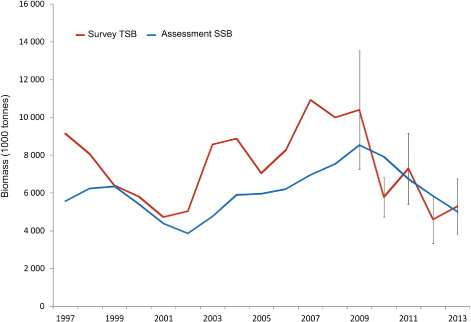
The estimates of herring density calculated here have sufficient precision to track cohorts over time reasonably well and the time series from the survey can be used to study trends in abundance of the stock. For instance, the downward trend in stock biomass from 2009 to 2013 is apparent. However, the precision is too low, causing too large a year-to-year variation for the estimates to be used as absolute values of stock abundance in one single year, and should therefore only be used as an index in the assessment.

In stock assessments based on VPA, currently the standard method employed by ICES for NSSH, it is generally assumed that the catch matrix of numbers at age is estimated without error (Shepherd 1999). In actuality, catch-at-age is estimated from multi-stage sampling surveys, and may have appreciable sampling errors because of low effective sample sizes caused by clustering effects (ICES 2013b). The primary sampling units are often defined by fishing operations or trips for at-sea sampling programmes, and port-days for on-shore sampling programmes (ICES 2013b). The VPA assessment model cannot appropriately account for sampling errors in the input data from the fisheries-dependent and fisheries-independent surveys and hence reliable estimates of the precision in estimates of SSB and F cannot be achieved. We therefore recommend that statistical assessment models (SAMs), which can account for sampling errors in input data from catch-at-age and survey indices by age group, should be tested by ICES for stock assessments of NSSH. The method proposed in this article may be used routinely to estimate sampling errors in abundance indices from the acoustic transect surveys. We also recommend that statistical methods based on best practice (ICES 2013b) should be used to estimate catch-at-age for NSSH, along with estimates of sampling errors. The model (Hirst et al. 2004, 2005, 2012), which is used by the Institute of Marine Research for estimating the catch-at-age of northeast Arctic cod and haddock, may also be applied to NSSH commercial fisheries data. If input data on catch-at-age and abundance indices are provided with sampling errors, then an SAM can be used to quantify the precision of the stock assessment (SSB and F). This would allow the determination of adequate sampling efforts in the IESNS and in sampling of commercial fisheries.

Editorial responsibility: Heino Fock

Acknowledgements

We greatly appreciate the comments from two reviewers, whose efforts helped to improve the manuscript.

Additional information

Funding

This work was supported by the Institute of Marine Research (IMR) and the Norwegian Research Council through the project ADMAR (Adaptive management of living marine resources by integrating different data sources and key ecological processes) (Project No. 200497/I30).

References

- Anon. 2010. Official Journal of the European Union, L 41/14. Commission Decision of 18 December 2009 adopting a multiannual Community programme for the collection, management and use of data in the fisheries sector for the period 2011–2013 (notified under document C(2009) 0121) (2010/93/EU). 64 pages.
- Cochran WG. 1977. Sampling Techniques. 3rd edition. New York: John Wiley and Sons. 428 pages.
- Efron B. 1982. The Jackknife, the Bootstrap and Other Resampling Plans. Philadelphia: Society of Industrial and Applied Mathematics (SIAM). 92 pages.
- Everson IM, Bravington M, Gossa I. 1996. A combined acoustic and trawl survey for efficiently estimating fish abundance. Fisheries Research 26:75–91.
- Foote KG, Knudsen HP, Vestnes G, MacLennan DN, Simmonds EJ. 1987. Calibration of acoustic instruments for fish density estimation: A practical guide. ICES Cooperative Research Report 144:1–57.
- Francis RICC. 1984. An adaptive strategy for stratified random trawl surveys. New Zealand Journal of Marine and Freshwater Research 18:59–71.
- Godø OR, Wespestad VG. 1993. Monitoring changes in abundance of gadoids with varying availability to trawl and acoustic surveys. ICES Journal of Marine Science 50:39–51.
- Harbitz A, Aschan M. 2003. A two-dimensional geostatistic method to simulate the precision of abundance estimates. Canadian Journal of Fisheries and Aquatic Sciences 60:1539–51.
- Harbitz A, Ona E, Pennington M. 2009. The use of an adaptive acoustic-survey design to estimate the abundance of highly skewed fish populations. ICES Journal of Marine Science 66:1349–54.
- Hirst D, Aanes S, Storvik G, Tvete IF. 2004. Estimating catch at age from market sampling data using a Bayesian hierarchical model. Journal of the Royal Statistical Society C: Applied Statistics 53:1–14.
- Hirst D, Storvik G, Aldrin M, Aanes S, Huseby RB. 2005. Estimating catch-at-age by combining data from different sources. Canadian Journal of Fisheries and Aquatic Sciences 62:1377–85.
- Hirst D, Storvik G, Rognebakke H, Aldrin M, Aanes S, Vølstad JH. 2012. A Bayesian modelling framework for the estimation of catch-at-age of commercially harvested fish species. Canadian Journal of Marine Science 69:2064–76.
- Hjelvik V, Handegard NO, Ona E. 2008. Correcting for vessel avoidance in acoustic-abundance estimates for herring. ICES Journal of Marine Science 65:1036–45.
- Holst JC, Røttingen I, Melle W. 2004. The herring. In: Skjoldal HR, Sætre R, Færno A, Misund OA Røttingen I, editors. The Norwegian Sea Ecosystem. Trondheim, Norway: Tapir Academic Press, p 203–26.
- ICES. 2009. Report of the PGNAPES Scrutiny of Echograms Workshop (WKECHO-SCRU), 16–18 February 2009, Bergen, Norway. ICES CM 2009/RMC:02. 20 pages.
- ICES. 2013a. Report of the Working Group on Widely Distributed Stocks (WGWIDE), 27 August–2 September 2013, Copenhagen, Denmark. ICES CM 2013/ACOM:15. 950 pages.
- ICES. 2013b. Report of the Second Workshop on Practical Implementation of Statistical Sound Catch Sampling Programmes, 6–9 November 2012, Copenhagen, Denmark. ICES CM 2012/ACOM:54. 71 pages.
- Jessen RJ. 1978. Statistical Survey Techniques. New York: John Wiley & Sons. 520 pages.
- Jolly GM, Hampton I. 1990. A stratified random transect design for acoustic surveys of fish stocks. Canadian Journal of Fisheries and Aquatic Sciences 47:1282–91.
- Korn EL, Graubard BI. 1998. Variance estimation for superpopulation parameters. Statistica Sinica 8:1131–51.
- Kotwicki S, De Robertis A, Ianelli JN, Punt A, Horne JK. 2012. Combining bottom trawl and acoustic data to model acoustic dead zone correction and bottom trawl efficiency parameters for semipelagic species. Canadian Journal of Fisheries and Aquatic Sciences 70:208–19.
- Lehtonen R, Pahkinen E. 2004. Practical Methods for Design and Analysis of Complex Surveys. 2nd edition. New York: John Wiley and Sons. 349 pages.
- Lumley T. 2010. Complex Surveys. A Guide to Analysis using R. New York: John Wiley & Sons. 276 pages.
- Løland A, Aldrin M, Ona E, Hjellvik V, Holst JC. 2007. Estimating and decomposing total uncertainty for survey-based abundance estimates of Norwegian spring-spawning herring. ICES Journal of Marine Science 64:1302–12.
- MacLennan DN, Fernandes PG, Dalen J. 2002. A consistent approach to definitions and symbols in fisheries acoustics. ICES Journal of Marine Science 59:365–69.
- Maravallias CD, Reid DG, Simmonds EJ. 1996. Spatial analysis and mapping of acoustic survey data in the presence of high local variability: Geostatistical application to North Sea herring (Clupea harengus). Canadian Journal of Fisheries and Aquatic Sciences 53:1497–505.
- McQuinn IH, Simrad Y, Stroud TWF, Beaulieu JL, Walsh SJ. 2005. An adaptive, integrated ‘acoustic-trawl’ survey design for Atlantic cod (Gadus morhua) with estimation of acoustic and trawl dead zones. ICES Journal of Marine Science 62:93–106.
- Nielsen A, Berg CW. 2014. Estimation of time-varying selectivity in stock assessments using state-space models. Fisheries Research 158:96–101.
- Ona E, Mitson RB. 1996. Acoustic sampling and signal processing near the seabed: The deadzone revisited. ICES Journal of Marine Science 53:677–90.
- Rose G, Gauthier S, Lawson G. 2000. Aquatic surveys in full monte: Simulating uncertainty. Aquatic Living Resources 13:367–72.
- Shepherd JG. 1999. Extended survivors analysis: an improved method for the analysis of catch-at-age data and abundance indices. ICES Journal of Marine Science 56:584–91.
- Simmonds EJ, Fryer RJ. 1996. Which are better, random or systematic acoustic surveys? A simulation using North Sea herring as an example. ICES Journal of Marine Science 53:39–50.
- Simmonds EJ, MacLennan D. 2005. Fisheries Acoustics: Theory and Practice. Oxford: Blackwell Science. 437 pages.
- Simmonds EJ, Gutierrez M, Chipollini A, Gerlotto F, Woillez M, Bertrand A. 2009. Optimizing the design of acoustic surveys of Peruvian anchoveta. ICES Journal of Marine Science 66:1341–48.
- Skaret G, Axelsen BE, Nøttestad L, Fernö A, Johannessen A. 2005. The behavior of spawning herring in relation to a survey vessel. ICES Journal of Marine Science 62:1061–64.
- Thorson JT, Clarke ME, Stewart IJ, Punt AE. 2013. The implications of spatially varying catchability on bottom trawl surveys of fish abundance: A proposed solution involving underwater vehicles. Canadian Journal of Fisheries and Aquatic Sciences 70:294–306.
- Tjelmeland S. 2002. A model for the uncertainty around the yearly trawl-acoustic estimate of biomass of Barents Sea capelin, Mallotus villosus (Müller). ICES Journal of Marine Science 59:1072–80.
- Toresen R, Gjøsæter H, de Barros P. 1998. The acoustic method as used in the abundance estimation of capelin (Mallotus villosus Müller) and herring (Clupea harengus Linné) in the Barents Sea. Fisheries Research 34:27–37.
- Totland A, Godø OR. 2001. BEAM – An interactive GIS application for acoustic abundance estimation. In: Nishida T, Kailola PR, Hollingworth CE, editors. Proceedings of the First Symposium on Geographic Information System (GIS) in Fisheries Science. Saitama, Japan: Fishery GIS Research Group, p 195–201.
- Walline PD. 2007. Geostatistical simulations of eastern Bering Sea walleye pollock spatial distributions, to estimate sampling precision. ICES Journal of Marine Science 64:559–69.
- Williams RL. 2000. A note on robust variance estimation for cluster-correlated data. Biometrics 56:645–46.
- Woillez M, Rivoirard J, Fernandes PG. 2009. Evaluating the uncertainty of abundance estimates from acoustic surveys using geostatistical simulations. Canadian Journal of Fisheries and Aquatic Sciences 66:1377–83.
- Wolter KM. 1985. Introduction to Variance Estimation. New York: Springer. 427 pages.