Applying photogrammetry to reconstruct 3D luminance point clouds of indoor environments

ABSTRACT

Computer-aided 3D modelling is the standard design method in the architecture, engineering, construction, owner, operator (AECOO) industry and in lighting design. Applying a photogrammetric process, a sequence of images is used to reconstruct the geometry of a space or an object in a 3D model. Likewise, a calibrated digital camera is utilized to measure the surface luminance values of an environment or an object. We propose a workflow in which the geometry and the luminance values are measured simultaneously by combining these two measurement methods. The pipeline has been assessed and validated through the application to a case study, the Aalto Hall (Aalto University, Espoo, Finland), in order to understand its potential.

KEYWORDS:

• photogrammetry
• photometry
• point cloud
• luminance
• 3d model
• indoor
• lighting

Introduction

In the architecture, engineering, construction, owner, operator (AECOO) industry, three-dimensional (3D) computer-aided modelling is applied to design in order to oversee construction and to maintain a building or built environment. Moreover, computer-aided 3D modelling is the standard method in lighting design (Roy, 2000; Shikder, Price, & Mourshed, 2009). Lighting distribution in an environment is a crucial attribute in both the ergonomics and the attractiveness of a space (Bellia, Bisegna, & Spada, 2011; Öztürk, 2003; So & Leung, 1998; Tiller & Veitch, 1995). In addition to occupant satisfaction, well-designed lighting can reduce the energy consumption of indoor lighting without compromising quality (Loe & Rowlands, 1996; Muhamad, Zain, Wahab, Aziz, & Kadir, 2010; Van Den Wymelenberg, Inanici, & Johnson, 2010). Architects and lighting designers need to understand the characteristics of existing lighting in order to design new lighting configurations (Rodrigue, Demers, & Parsaee, 2020).

Our aim is to develop and present (through a case study) a process allowing both the 3D reconstruction of interior geometry and luminance mapping from the same image set. In other words, by applying photogrammetry we reconstruct a 3D luminance point cloud and present the measuring of a 3D luminance map in indoor environments. Section 2 describes the principles of the imaging luminance photometry and photogrammetric reconstruction relevant to this article. In Section 3, Materials and methods, the workflow is illustrated with particular attention to the combination of imaging luminance photometry and photogrammetry. In addition, the indoor space specifications of our case study are presented in Section 3. The Results section shows the outcomes of our method: the luminance image locations and orientations, the 3D surface model and the 3D luminance point cloud. The luminance values in the created luminance point cloud and single luminance images are compared, and their differences listed. In the Discussion section, we discuss the potential of a luminance point cloud when used in lighting assessment and visualization and propose possible further research.

Related work

The human eye and the visual system adapt to lighting conditions via a variety of mechanisms. The luminance distribution of a visual environment governs the level of adaptation in the observer’s retina. The adaptation luminance in the field of view affects contrast sensitivity, visual acuity, accommodation, pupillary contraction and eye movements. Furthermore, the luminance distribution also affects certain aspects of visual comfort such as glare sensitivity, visual fatigue and dullness due to a visually non-stimulating environment (CEN, 2002).

The luminances of a space can be measured point-by-point by employing a spot luminance metre. For a thorough analysis of luminance distribution, however, the point-by-point method is not pragmatic. Hence, a commonly used method for luminance distribution measurement is imaging luminance photometry (Borisuit, Scartezzini, & Thanachareonkit, 2010; Hiscocks & Eng, 2011; Rea & Jeffrey, 1990). In imaging luminance photometry, a radiometrically calibrated digital camera is used to capture the luminance values of a measurement area in an image or series of images. Even though the measured spaces are three dimensional, the measurement images are only two dimensional. This limits the applicability of imaging luminance photometry in spatial analyses and creates data management issues if larger environments are studied.

The history of image-based 3D building measurement (i.e. architectural photogrammetry) is nearly as old as photography itself (Albota, 1976). From the 1990s, digital photogrammetry enabled automatic image measurements, camera calibration and exterior orientation (Haggrén & Niini, 1990; Heikkilä & Silven, 1997; Lowe, 1999; Pollefeys, Koch, & Van Gool, 1999; Stathopoulou, Welponer, & Remondino, 2019). Current photogrammetric software can automatically reconstruct 3D mesh models (Furukawa, Curless, Seitz, & Szeliski, 2009; Jancosek & Pajdla, 2011; Romanoni, Delaunoy, Pollefeys, & Matteucci, 2016). For indoor modelling, various photogrammetric methods have been used, such as 3D mapping systems (El-Hakim, Boulanger, Blais, & Beraldin, 1997), videogrammetry-based 3D modelling (Haggrén & Mattila, 1997), structured indoor modelling (Ikehata, Yang, & Furukawa, 2015), cloud-based indoor 3D modelling (Ingman, Virtanen, Vaaja, & Hyyppä, 2020) and other indoor measuring methods (Georgantas, Brédif, & Pierrot-Desseilligny, 2012; Lehtola et al., 2017; León-Vega & Rodríguez-Laitón, 2019). In addition, high dynamic range (HDR) photogrammetry has been used for luminance mapping of the sky and the sun (Cai, 2015) and a laser-scanned point cloud have been coloured with luminance values in a nighttime road environment (Vaaja et al., 2015; Vaaja et al., 2018).

While both imaging luminance measurement and indoor 3D reconstruction have been extensively presented with conventional digital cameras in prior research, their integration remains to be demonstrated. Laser scanning and HDR imaging have been proposed for surveying and visualizing lighting in indoor spaces, since current lighting measurement methods are too limited for 3D design (Rodrigue et al., 2020). The study also showed that the characteristics of the existing lighting need to be understood by architects and lighting designers in order to redesign the lighting. However, when Rodrigue et al. (2020) performed such measurements, they only transmitted the colour values for visual inspection of the 3D point cloud, as the values were obtained from an uncalibrated scanner camera and not from a luminance-calibrated camera. In addition, their research revealed that 2D luminance photometry alone is not appropriate for surveying an indoor space with six degrees of freedom, and image locations must be managed manually. Since the geometry and the luminance maps remain in separate data sets, the use of the data is impractical. Therefore, the current research gap is the integration and the simultaneous execution of luminance imaging and photogrammetric 3D reconstruction, and the automatic management of image locations and orientations. Furthermore, the main 3D reconstruction software, such as Agisoft Metashape,¹ COLMAP,² iWittnessPRO,³ Meshroom,⁴ RealityCapture,⁵ VisualSFM⁶ and WebODM⁷, cannot be conveniently applied to create a 3D luminance model. The main inconvenience is the inflexibility of the usable bit-depth (8 bits) in 3D reconstruction software, and the bit-depth (16 bits) needed to preserve the dynamic resolution of luminance imaging. Hiscocks (2016) presents instructions on how to calibrate a camera in terms of photometry using open source software (Luma⁸). However, following the mentioned instructions and using Luma requires more or less the same knowledge and experience as performing the calibration and creating the luminance image management software by oneself. Hence, the 3D luminance measurement is not currently an easily approachable technology for professionals such as architects and lighting designers. Obviously, 3D luminance can be simulated when using CAD models or building information models (BIMs) (Foldbjerg et al., 2012). However, CAD models or BIMs of old buildings are not always available. Moreover, there exist several software solutions for lighting calculation and lighting design (e.g. AGi32,⁹ AutoLUX,¹⁰ DiaLUX,¹¹ Radiance,¹² Relux¹³).

Principles of luminance imaging and photogrammetric reconstruction

Luminance imaging

Imaging luminance photometry refers to capturing the two-dimensional (2D) presentation of an environment. The photometry is performed by applying a digital camera that has been radiometrically calibrated (Anaokar & Moeck, 2005; Hiscocks & Eng, 2013; Meyer, Gibbons, & Edwards, 2009; Wüller & Gabele, 2007). Hence, each picture element presents an individual luminance value of the measured scene. The digital R, G and B pixel values can be interpreted as relative luminance values when applying Equation 1 (IEC, 1999): (1) $L_r=0.2126R+0.7152G+0.0722B.$(1) The relative luminance, L_r, can be converted into absolute luminance (cd/m²) by applying a calibration constant. The calibration constant is unique for each camera, and it can be achieved by calibrating the camera using a reference luminance source. Furthermore, the vignetting of the camera must be solved as part of the luminance calibration (Kurkela et al., 2017).

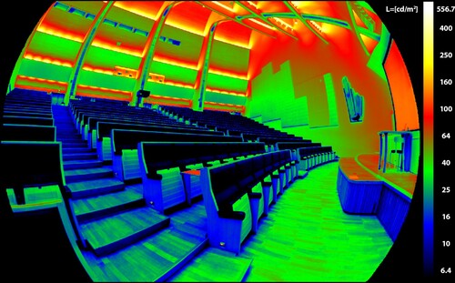
There are commercial imaging luminance photometers such as TechnoTeam LMK Mobile Advanced.¹⁴ Figure 1 presents a screenshot of a pseudo-coloured luminance measurement from TechnoTeam LMK LabSoft¹⁵ software. However, none of the commercial luminance imaging solutions were applicable for this study, as we needed complete control throughout the image processing. Hence, we used a camera which we calibrated ourselves, and we programmed all of the luminance image processing ourselves.

Figure 1. A pseudo-coloured luminance mapping measured with an imaging luminance photometer (LMK LabSoft). The legend shows the absolute luminance values (in cdm⁻²) on a logarithmic scale.

Photogrammetric reconstruction

Photogrammetry can be defined as a set of methods for interpreting and measuring images that can be used to determine the shape of an object and the location of images taken of the object (Luhmann, Robson, Kyle, & Harley, 2006, p. 2).

Figure 2 shows the simplified photogrammetric reconstruction process. The first task after image capturing is to identify the characteristic features P_n,m that describe the objects within the picture. For this purpose, the most common algorithm is the scale invariant feature transform (SIFT), which recognizes scale-invariant features in an image (Lowe, 1999). The features identified in the input images are used as reference elements in order to recognize the same objects within different images; therefore, the matching is realized first among features and, consequently, between images.

Figure 2. The principal procedures of close range photogrammetry. The dotted line indicates the connection between image features P_n,m, external image orientations R_n,t_n and the tie point P₁.

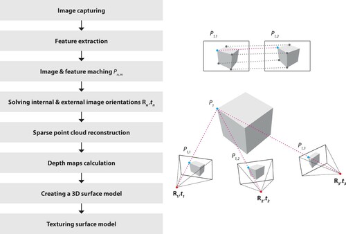
Solving internal and external image orientations is the step that determines the relationship between image observations P_n,m and the 3D points P_n of the object. External orientation determines the orientation and position of the camera in the global coordinate system. The rotation matrix R defines the angular orientation and the vector t is the spatial position of the camera.

Interior orientation represents the intrinsic geometric properties of the camera and the lens system. The parameters of interior orientation illustrate the position of the perspective centre, the focal length and the location of the principal point. The lens system causes errors in the image, which compensates for major geometric distortions such as radial and tangential distortions. The sensor deviations are corrected for affinity and shear, which represent the orthogonality of the image plane and the scale of the image coordinates (e.g. Brown, 1971; Fryer & Brown, 1986; Heikkilä, 2000).

The process of solving internal and external image orientations is iterative and usually begins with the orientation of a pair of images and the reconstruction of the scene (Nister, 2004). By increasing the number of images, the orientation of other images will also be solved. The orientations are approximate and the results are improved by using a bundle adjustment that optimizes the external and internal orientation of all images as well as the sparse point cloud consisting of the tie point P_n (e.g. Brown, 1976). The scale can be determined by measuring the distance between two measured points P_n.

There are several methods and algorithms that can be used to reconstruct a high detail 3D surface model. For example, it can be retrieved directly from the depth maps (Furukawa et al., 2009) or from the sparse point cloud. However, such a model is often an insufficient representation of reality because it lacks information. Otherwise, a dense point cloud can be used. In all these alternatives, a depth map is reconstructed for all oriented images (i.e. a depth value is determined for each pixel) using methods such as Semiglobal Matching (SGM) (Hirschmuller, 2008) or AD-Census (Mei et al., 2011). In addition, the tetrahedralization method proposed by Jancosek and Pajdla (2011) can be adopted because it performs well for reconstructing large, uniform, and mono-coloured surfaces. Finally, the 3D model is textured.

Materials and methods

Camera equipment and image data

As the aim was to facilitate both luminance mapping and 3D reconstruction from the same image set, the requirements from both of these had to be taken into account in data acquisition. Imaging luminance photometry is usually accomplished by capturing multiple images from one location using a tripod. Photogrammetric imaging is performed by capturing images from different locations and a tripod could be used especially for low lighting situations. In our case, however, the complex environment would have made the use of a tripod inconvenient and time-consuming. Hence, we captured the image set with a hand-held camera. As the optimal camera system and settings for these two measurement methods differ, a compromise is needed. In practice, this means that the exposure is determined by the lowest luminance value we want to measure, and using HDR imaging was not applicable.

We used a Nikon D800E camera with a Nikkor AF-S 14-24 mm f/2.8G ED lens locked to a 14 mm focal length. For hand-held image capturing, we applied a 1/250 s shutter speed. The aperture of f/5.6 and the ISO sensitivity of 3,200 were selected for optimal depth of field and signal-to-noise ratio. The camera had been calibrated both radiometrically and geometrically, and the vignetting correction function for the camera system was determined (Kurkela et al., 2017).

The full measurement data set consisted of 453 Nikon electronic format (NEF) raw images. The adopted 3D reconstruction software slightly altered the 16-bit images, while the 8-bit images remain unchanged. Hence, the following pre-processing was performed on the measurement series in order to preserve its bit depth when using 8-bit images. The luminance information is a single scalar that is obtained from the measured R, G, and B values by applying Equation 1. The original bit depth of the raw measurement was between 12 and 13 bits, which was converted to a 16-bit image for luminance calculation. In the photogrammetric reconstruction, we had three 8-bit channels – R, G and B – that we could use for each 16-bit luminance scalar. Hence, the single 16-bit luminance information was mapped over the three 8-bit channels. In this way, the usable dynamic range of 3 * 8-bits was attained, with the ability to distinguish 2²⁴ different numeric values. Thus, the dynamic resolution of the image (approximately 13 bits) can be preserved through the 3D reconstruction process.

Workflow for 3D luminance mapping

The workflow (see Figure 3) includes the documentation of the luminance image locations and orientations, the 3D surface model and the 3D luminance mapping.

Figure 3. The workflow for producing (a) image locations and orientations, (b) the 3D surface model and (c) the luminance point cloud.

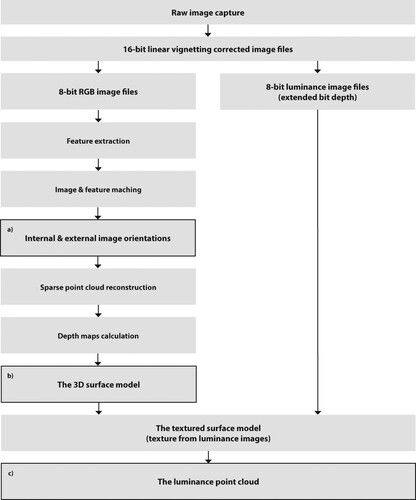
Images captured in the NEF image format were developed into linear 16-bit TIFF images using the DCRaw¹⁶ image processing programme. In the conversion, the Nikon raw colour space was used, and the pixels were interpolated using adaptive homogeneity-directed (AHD) interpolation. We corrected vignetting, and then the processing branched into the photogrammetry part and the luminance photometry part (Figure 3). The 16-bit images were processed in two different 8-bit versions. For the photogrammetric image version, the RGB images were processed so that as many feature points as possible were identified. For the luminance photometry image version, the 16-bit linear RGB images were transformed into monochromatic relative luminance images by applying Equation 1. The 16-bit monochromatic luminance data was coded over the three 8-bit RGB channels of an 8-bit image to obtain the extended bit depth, as described in Section 3.1 (Camera equipment and image data).

Agisoft Metashape software version 1.6.0.9925 was utilized for the 3D reconstruction (Figure 3). Internal and external image orientations were solved using the following alignment parameters: accuracy was set to ‘highest’, generic preselection was used, and the tie point limit was set to 100,000. For internal orientation, optimization parameters focal length (f), principal point coordinates (cx, cy), radial distortion coefficients (k1, k2, k3) and tangential distortion coefficients (p1, p2) were used.

In Agisoft Metashape, there are three methods to reconstruct a surface mesh model: directly from the sparse cloud, using the dense cloud and using the depth maps. We created the 3D surface model by applying the depth maps based mesh reconstruction method (Agisoft Metashape User Manual¹⁷). Depth map generation parameters were set ‘ultra high quality’ with ‘mild filtering’. At this point, a dense mesh model textured with the RGB images was exported for visual assessment. However, the exported RGB 3D model was not used for creating the luminance point cloud. Instead, the RGB images used for 3D reconstruction were replaced with the luminance images (see Figure 3). The surface model was textured with luminance images using the blending mode value: average, which uses the weighted average value of all pixels from individual photos. The mesh model textured with the luminance images was exported from Agisoft Metashape in the.obj format. The model was opened with CloudCompare¹⁸ version 2.9.1 and sampled into a point cloud using the Sample Points tool. The point cloud was exported as a text file in the format XYZRGB. The text file was processed by a Python programme written by us. For each point, a 16-bit relative luminance value was calculated from the R, G and B values. An absolute luminance value was calculated from each relative luminance value by applying the luminance calibration constant. The constant was obtained by capturing images of an Optronic Laboratories, Inc., model 455–6–1 reference luminance source’s exit port. The luminance value of the exit port was simultaneously measured with a Konica Minolta CS-2000 spectroradiometer. Finally, the luminance calibration constant was achieved by comparing the camera measurement to the spectroradiometer measurement. Each calculated absolute luminance value was stored as a scalar for each 3D point, and the point cloud was saved in the format XYZL, where L is the absolute luminance value. The luminance point cloud visualizations were created in CloudCompare.

Case study

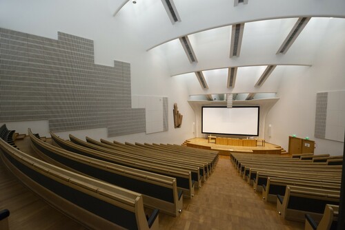
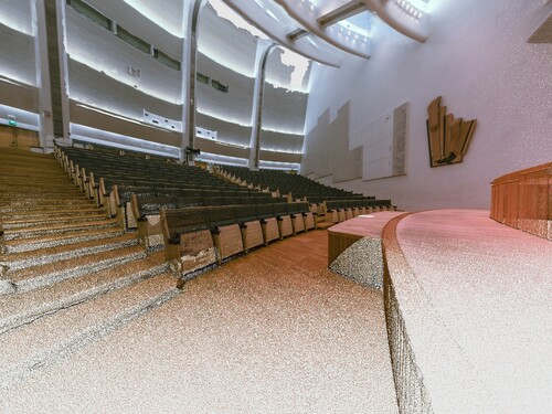
In the presented case, the measured space is a lecture hall (Aalto Hall, Aalto University, Espoo, Finland), designed by architect Alvar Aalto. This interior and the entire building are considered culturally valuable and are protected under the Finnish Act on the Protection of the Built Heritage. The protection implies that any altering of the space is strictly regulated. However, the light sources can be updated as better lighting technologies emerge and the original light sources are no longer available. Due to the geometry of the space (see Figure 4), both its geometry and lighting can be considered difficult to measure. The area of Aalto Hall is 493 m², and the maximum allowed number of persons inside is 570.

Figure 4. The measured lecture hall.

Results

Luminance image location documentation

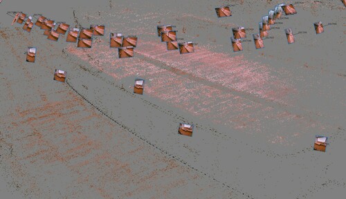
When applying the photogrammetric reconstruction workflow described in Section 3.2 (Workflow for 3D luminance mapping), the locations and orientations of the captured images were archived as metadata. This was executed in the internal and external camera orientation phase of the photogrammetric process, as illustrated in Figure 3. Figure 5 shows the 145,301 tie points used for camera alignment at which the 453 images were captured. Luminance images incorporated the same internal and external orientations as the RGB images captured for photogrammetric reconstruction.

Figure 5. The tie points used for camera alignment.

The reconstructed 3D surface model

Figure 6 shows the 3D surface model reconstructed from RGB images. The 3D model was reconstructed using 453 images in Agisoft Metashape. The mesh density varied considerably, depending on the number of unique features in the surface texture. Table 1 shows information about the 3D model. Figure 7 illustrates a detail from the textured surface model.

Figure 6. The textured 3D surface model.

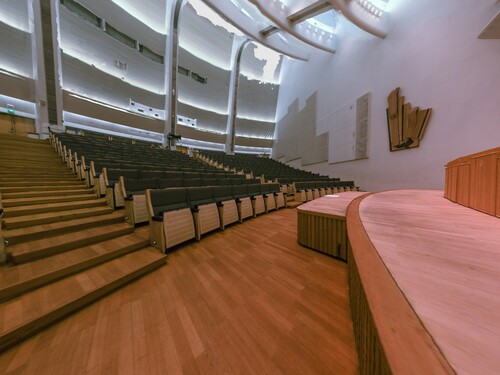
Figure 7. A detail from the textured surface model shown both without texture (left) and with image texture (right).

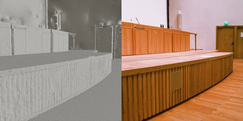
Table 1. The processing parameters.

Number of images	453
Tie points	145,301
Faces	21,655,220
Vertices	10,827,683
Texture size (pixels)	4,096 × 4,096
Texture count	16

The luminance point cloud

The pseudo-coloured luminance point cloud

Figure 8 presents the luminance point cloud of the measurement area. Luminance point clouds were utilizable for visualizing or analyzing the luminance distribution of an interior in 3D, and the pseudo-colours represented the absolute luminance value range of 0.0–1142.1 cd/m².

Figure 8. A luminance point cloud.

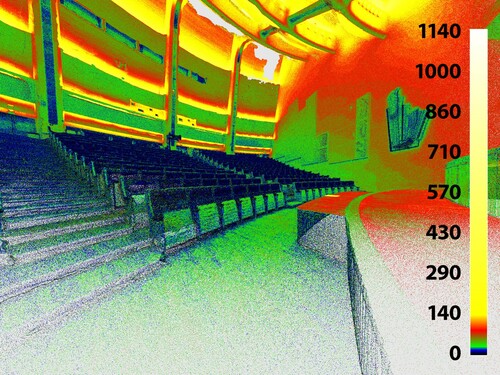
The luminance point cloud was sampled from the textured surface model and consisted of 100,002,877 points. Hence, the point density of the point cloud had an even distribution of approximately 80,000 points per square metre. Every point in the point cloud was coloured with its respective luminance value, as described in Section 3.2 (Workflow for 3D luminance mapping).

Figure 9 illustrates the RGB point cloud of the measurement area. The point cloud contains both the luminance values and the RGB presentation. Switching between the luminance and RGB presentations assists in visual lighting assessment.

Figure 9. An RGB point cloud.

Quantifiable comparison of the reflective surface

During the 3D reconstruction of the measured environment, both the geometry and the radiometry are approximated to a certain extent. In order to assess the correspondence between single-image luminance measurements and the reconstructed luminance point cloud, seven surface areas (areas A to G) were chosen. Figure 10 illustrates the areas. As the measurement image set consisted of 453 images, each surface area existed in tens of images. We chose to present three single measurements per surface area selected from different measurement locations. Table 2 presents the luminance values from single measurements from the luminance point cloud and the relative differences between the average luminance in three single images and the point cloud. The luminance values of the single images were used as the ground truth to which the luminance values of the point cloud were compared.

Figure 10. The luminance measurement areas A to G.

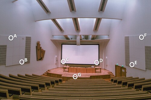
Table 2. The median luminance values measured from the selected reference areas and analyzed for single images and the reconstructed point cloud.

	Single image median luminance and their average (cdm^−2)				Median luminance in the equivalent point cloud region (cdm^−2)	Relative difference between the average luminance of three single images and the point cloud
A	72.33	69.10	64.89	68.77	79.80	16.0%
B	57.99	56.06	55.45	56.50	64.63	14.4%
C	155.86	158.80	154.55	156.40	148.17	5.3%
D	135.33	140.07	133.47	136.29	132.97	2.4%
E	57.81	59.68	53.16	56.88	64.63	13.6%
F	69.95	71.73	60.90	67.53	72.17	6.9%
G	203.64	205.06	193.07	200.59	193.79	3.4%
						Average: 8.9%

Discussion

We presented simultaneous imaging luminance photometry and photogrammetry applied to an indoor space through a case study and the 3D luminance point cloud created from the measurement. The 3D reconstruction automatically created documentation of the imaging luminance measurements where the positions and the orientations of the camera were placed in a 3D point cloud, as described in Section 3.2 (Workflow for 3D luminance mapping). The measured luminance values remained constant through the 3D reconstruction with satisfactory confidence. The absolute luminance values of the reconstructed 3D point cloud were similar to the values in the single luminance images of the calibrated camera, with an average relative difference of 8.9%.

The presented 3D luminance mapping methods offer several potential benefits for the AECOO industry. As the presented method constitutes both geometric reconstruction and luminance mapping, the method can also be applied in cases where no pre-existing 3D digital documentation is available. Therefore, 3D luminance mapping is also compatible with buildings for which BIMs, do not exist. Hence, the method can also be applied with older buildings and, for example, cultural heritage sites that may not have any up-to-date digital documentation available. In such cases, the evaluation of current lighting conditions can be carried out without needing a full building survey by terrestrial laser scanning and manual modelling of the existing building. For complex sites, the manual modelling may alone require several weeks of working time (e.g. Kersten et al., 2017), making lighting estimation via 3D modelling and simulation rather inefficient. Potentially, the presented method can simultaneously serve the needs of the 3D documentation of building geometry and mapping the lighting conditions, leading to further cost savings via the use of more affordable instruments. In comparison with TLS, close range photogrammetry utilizing Agisoft Metashape has been found to be feasible for the 3D documentation of the built environment (Kersten, Mechelke, & Maziull, 2015). As the photogrammetric reconstruction simultaneously solves the imaging locations, they can also be included in the building documentation and queried according to the position, thus simplifying data management in projects. Furthermore, applying a luminance-calibrated camera does not necessarily increase the workload of photogrammetric measurement, and the luminance calculations can be implemented in the photogrammetric reconstruction process without a significant increase in computing time.

In retrofitting projects, the method allows for the verification of the existing lighting systems’ performance, and identification of the most significant problem areas in the building, where modifications to the lighting system have to be considered. This can support energy savings via the use of natural light (Gago, Muneer, Knez, & Köster, 2015) or an estimation of visual comfort (Konis, 2013). Future work should address the approach in a real-life AECOO scenario and measure the amount of time and money that could be saved during the retrofitting phase of the building (e.g. installing new windows or lights in a specific area).

Large, smooth, uniform and mono-coloured surfaces are problematic to capture and reconstruct accurately with photogrammetry (Lehtola, Kurkela, & Hyyppä, 2014). Such surfaces lack the unique features that are essential for photogrammetric reconstruction. In addition, obstructed and dark areas can be difficult to reconstruct. Good measurement practices can help these problems to a certain extent. By ensuring sufficient and diffuse illumination, the measurer can use a low ISO value with a digital camera in order to have as high a signal-to-noise ratio as possible. In the case of 3D lighting measurement, however, lighting cannot be adjusted. The best practices should ensure the presence of each feature in two or more input images. A tripod could be used when capturing the whole photogrammetric image series, but this would be slow and impractical.

Large uniform surfaces are convenient to measure with a laser scanner, if such a device is available. Compared to photogrammetry, laser scanning benefits from better measuring accuracy and precision on flat and featureless surfaces and from direct scale determination, among other things. Laser scanning is an active measuring method that emits either visible or infrared radiation, and thus it cannot solely be used in measuring luminance. Moreover, laser scanners often include a digital camera for colouring the scanned point clouds. If the camera in the laser scanner is controllable and luminance is calibrated, it is possible to capture luminance point clouds with the scanner; otherwise the luminance measurements can only be used for visual inspection of the 3D point cloud if an uncalibrated scanner camera is used. Nevertheless, photogrammetric reconstruction combined with laser scanning benefits from the advantages of both methods (Julin et al., 2019). These benefits include the dimensional accuracy of laser scanning and the dynamic range and resolution of photogrammetry. Presumably, the integration of laser scanning and photogrammetry is even a necessity, unless all of the surfaces of the measurement environment have features that are suitable in terms of photogrammetry. Hence for future research, we strongly recommend considering laser scanning as a part of 3D luminance measurement.

It is possible to integrate the presented 3D reconstruction method into conventional indoor luminance measurements as they are described in CEN or IES measurement standards or guidelines (CEN, 2002; IES, 2014). In such an integration, the 3D model works as a catalogue of luminance measurements performed from the locations and measurement directions according to the guidelines. Moreover, HDR measurement for glare assessment is also possible in this scenario. Obviously, this would require a lot of front-end software development, as no current off-the-shelf 3D reconstruction software is especially designed for luminance measurement. A possible topic for further research could include a hybrid method approach, where the luminance and HDR glare measurements are taken from a tripod following the standardized measurement guidelines, and the same imaging luminance photometer is used for non-HDR photogrammetry. In this way, it is possible to obtain the standardized measurements in order to register the 3D point cloud and to perform the photogrammetry in a pragmatic time frame.

Conclusions

In this study, we presented a workflow where photogrammetric 3D reconstruction and imaging luminance photometry are performed from the same image set captured with a luminance-calibrated camera. Furthermore, we demonstrated the workflow via a case study. We assessed the luminance data quality of the created luminance point cloud by comparing the luminance values in the point cloud to single luminance images used as ground truth data. The relative average difference between the luminance point cloud and the single luminance images was 8.9%. Both 3D measurement and reality-based 3D modelling are spreading from a niche position to various forms of applications. The workflow introduced in this article could already be repeated with low-cost equipment such as compact cameras. In even more open-ended predictions of the future, we will hopefully see nighttime 3D city models in addition to today’s daytime models. For creating such nighttime 3D city models, the authors believe that luminance photogrammetry could certainly be a utilizable method. Even though this research focused on indoor applications, the presented workflow can be generalized for various 3D lighting measuring and modelling concepts.

Disclosure statement

No potential conflict of interest was reported by the author(s).

Additional information

Funding

This work was supported by the Academy of Finland – Strategic Research Council under Grant [No. 293389, 314312].

Notes

1 Agisoft Metashape. Agisoft. Available at: https://www.agisoft.com/ (accessed February 4, 2020)

2 COLMAP. Johannes L. Schoenberger. Available at: https://colmap.github.io/ (accessed August 28, 2020)

3 iWittnessPRO. Photometrix Photogrammetry Software. Available at: https://www.photometrix.com.au/ (accessed August 28, 2020)

4 Meshroom. ALICEVISION association. Available at: https://alicevision.org/ (accessed August 28, 2020)

5 RealityCapture. Capturing Reality s.r.o. Available at: https://www.capturingreality.com/ (accessed February 4, 2020)

6 VisualSFM. Changchang Wu. Available at: http://ccwu.me/vsfm/ (accessed August 28, 2020)

7 WebODM. OpenDroneMap. Available at: https://www.opendronemap.org/ (accessed August 28, 2020)

8 LUMA: Luminance Analysis. Syscomp Electronic Design Limited. Available at: https://www.ee.ryerson.ca/~phiscock/astronomy/luma/luma-58.zip (accessed August 28, 2020)

9 AGi32. Lighting Analysts. Available at: https://lightinganalysts.com/ (accessed August 28, 2020)

10 AutoLUX. Keysoft Solutions. Available at: https://www.keysoftsolutions.co.uk/bim-products/keysoft-traffic/keylights/ (accessed August 28, 2020)

11 DIALux. DIAL. Available at: https://www.dial.de/en/home/ (accessed August 28, 2020)

12 Radiance. Lawrence Berkeley National Laboratory. Available at: https://www.radiance-online.org/ (accessed August 28, 2020)

13 Relux. Relux Informatik AG. Available at: https://relux.com/en/ (accessed August 28, 2020)

14 TechnoTeam LMK Mobile Advanced. TechnoTeam Bildverarbeitung GmbH. Available at: https://www.technoteam.de/apool/tnt/content/e5183/e5432/e5733/e5736/LMK_mobile_manual_EOS550D_eng.pdf (accessed February 4, 2020)

15 LMK LabSoft. TechnoTeam Bildverarbeitung GmbH. Available at: https://www.technoteam.de/product_overview/lmk/software/lmk_labsoft/index_eng.html (accessed February 4, 2020)8.

16 DCRaw. Dave Coffin. Available at: https://www.dechifro.org/dcraw/ (accessed February 4, 2020)

17 Agisoft Metashape User Manual: Professional Edition, Version 1.6. 2020 Agisoft LLC. Available at: https://www.agisoft.com/pdf/metashape-pro_1_6_en.pdf (accessed October 25, 2020)

18 CloudCompare. CloudCompare project. Available at: http://www.cloudcompare.org/ (accessed February 4, 2020)

References

- Albota, M. G. (1976). Short chronological history of photogrammetry. Proceedings of XIII Congress of the International Society for Photogrammetry. Commission VI, Helsinki, (pp. 20).
- Anaokar, S., & Moeck, M. (2005). Validation of high dynamic range imaging to luminance measurement. Leukos, 2(2), 133–144. doi:https://doi.org/10.1582/LEUKOS.2005.02.02.005
- Bellia, L., Bisegna, F., & Spada, G. (2011). Lighting in indoor environments: Visual and non-visual effects of light sources with different spectral power distributions. Building and Environment, 46(10), 1984–1992. doi:https://doi.org/10.1016/j.buildenv.2011.04.007
- Borisuit, A., Scartezzini, J.-L., & Thanachareonkit, A. (2010). Visual discomfort and glare rating assessment of integrated daylighting and electric lighting systems using HDR imaging techniques. Architectural Science Review, 53(4), 359–373. doi:https://doi.org/10.3763/asre.2009.0094
- Brown, D. C. (1971). Close-range camera calibration. Photogrammetric Engineering, 37(8), 855–866.
- Brown, D. C. (1976). The bundle adjustment-progress and prospect. Proceedings of XIII Congress of the International Society for Photogrammetry. Commission VI, Helsinki.
- Cai, H. (2015). Using high dynamic range photogrammetry for luminance mapping of the Sky and the Sun. AEI 2015: Birth and Life of the Integrated Building, doi:https://doi.org/10.1061/9780784479070.029
- CEN - EN 12464-1. (2002). Light and lighting - lighting of work places - Part 1: Indoor work Places. European Committee for Standardization. Brussels.
- El-Hakim, S. F., Boulanger, P., Blais, F., & Beraldin, J. A. (1997). System for indoor 3D mapping and virtual environments. Videometrics V, 3174, 21–35. International Society for Optics and Photonics. doi:https://doi.org/10.1117/12.279791
- Foldbjerg, P., Asmussen, T. F., Roy, N., Sahlin, P., Ålenius, L., Jensen, H. W., & Jensen, C. (2012). Daylight Visualizer and Energy & Indoor Climate Visualizer, a Suite of Simulation Tools for Residential Buildings. Proceedings of the building simulation and optimization conference BSO12, Loughborough, September.
- Fryer, J. G., & Brown, D. C. (1986). Lens distortion for close-range photogrammetry. Photogrammetric Engineering and Remote Sensing, 52(1), 51–58.
- Furukawa, Y., Curless, B., Seitz, S. M., & Szeliski, R. (2009). Reconstructing building interiors from images. 2009 IEEE 12th International Conference on Computer Vision, (pp. 80–87). IEEE. doi:https://doi.org/10.1109/ICCV.2009.5459145
- Gago, E. J., Muneer, T., Knez, M., & Köster, H. (2015). Natural light controls and guides in buildings. Energy saving for electrical lighting, reduction of cooling load. Renewable and Sustainable Energy Reviews, 41, 1–13. doi:https://doi.org/10.1016/j.rser.2014.08.002
- Georgantas, A., Brédif, M., & Pierrot-Desseilligny, M. (2012). An accuracy assessment of automated photogrammetric techniques for 3D modelling of complex interiors. International Archives of the Photogrammetry, Remote Sensing and Spatial Information Sciences, 39, 23–28.
- Haggrén, H., & Mattila, S. (1997). 3D indoor modeling from videography. Videometrics V, 3174, 14–20. International Society for Optics and Photonics. doi:https://doi.org/10.1117/12.279781
- Haggrén, H., & Niini, I. (1990). Relative orientation using 2D projective transformations. The Photogrammetric Journal of Finland, 12(1), 22–23.
- Heikkilä, J. (2000). Geometric camera calibration using circular control points. IEEE Transactions on Pattern Analysis and Machine Intelligence, 22(10), 1066–1077. Oct. 2000. doi:https://doi.org/10.1109/34.879788
- Heikkilä, J., & Silven, O. (1997). A four-step camera calibration procedure with implicit image correction. Proceedings of IEEE computer society conference on computer vision and pattern recognition, (pp. 1106–1112). IEEE. doi:https://doi.org/10.1109/CVPR.1997.609468
- Hirschmuller, H. (2008). Stereo processing by Semiglobal Matching and Mutual Information. IEEE Transactions on Pattern Analysis and Machine Intelligence, 30(2), 328–341. February. doi:https://doi.org/10.1109/TPAMI.2007.1166
- Hiscocks, P. D. (2016). LUMA: Luminance Analysis Software Manual. Syscomp electronic design limited. https://www.ee.ryerson.ca/~phiscock/astronomy/luma/luma-manual-0.3.pdf
- Hiscocks, P. D., & Eng, P. (2011). Measuring luminance with a digital camera. Syscomp electronic design limited. https://www.atecorp.com/atecorp/media/pdfs/data-sheets/Tektronix-J16_Application.pdf
- Hiscocks, P. D., & Eng, P. (2013). Measuring luminance with a digital camera: case history. https://www.ee.ryerson.ca/~phiscock/astronomy/light-pollution/luminance-case-history.pdf
- IEC. (1999). 61966-2-1: 1999 Multimedia systems and equipment-colour measurement and management-Part 2-1: Colour management-Default RGB colour space-sRGB. International Electrotechnical Commission. Geneva.
- IES - ANSI/IES RP-3-13. (2014). American National standard practice on lighting for educational facilities. Illuminating Engineering Society. New York.
- Ikehata, S., Yang, H., & Furukawa, Y. (2015). Structured indoor modeling. Proceedings of the IEEE International Conference on Computer Vision, (pp. 1323–1331).
- Ingman, M., Virtanen, J.-P., Vaaja, M. T., & Hyyppä, H. (2020). A comparison of low-cost sensor systems in automatic cloud-based indoor 3D Modeling. Remote Sensing, 12(16), 2624. doi:https://doi.org/10.3390/rs12162624
- Jancosek, M., & Pajdla, T. (2011). Multi-view reconstruction preserving weakly-supported surfaces. CVPR, 2011, 3121–3128. IEEE. doi:https://doi.org/10.1109/CVPR.2011.5995693
- Julin, A., Jaalama, K., Virtanen, J.-P., Maksimainen, M., Kurkela, M., Hyyppä, J., & Hyyppä, H. (2019). Automated multi-sensor 3D reconstruction for the web. ISPRS International Journal of Geo-Information, 8(5), 221. doi:https://doi.org/10.3390/ijgi8050221
- Kersten, T. P., Büyüksalih, G., Tschirschwitz, F., Kan, T., Deggim, S., Kaya, Y., & Baskaraca, A. P. (2017). The Selimiye Mosque of Edirne, Turkey – an immersive and interactive virtual reality experience using HTC Vive. The International Archives of the Photogrammetry, Remote Sensing and Spatial Information Sciences, XLII-5/W1, 403––409. doi:https://doi.org/10.5194/isprs-archives-XLII-5-W1-403-2017
- Kersten, T., Mechelke, K., & Maziull, L. (2015). 3D model of al zubarah fortress in Qatar—Terrestrial laser scanning vs. dense image matching. The International Archives of Photogrammetry, Remote Sensing and Spatial Information Sciences, 40(5), 1–8. doi:https://doi.org/10.5194/isprsarchives-XL-5-W4-1-2015
- Konis, K. (2013). Evaluating daylighting effectiveness and occupant visual comfort in a side-lit open-plan office building in San Francisco, California. Building and Environment, 59, 662–677. doi:https://doi.org/10.1016/j.buildenv.2012.09.017
- Kurkela, M., Maksimainen, M., Vaaja, M. T., Virtanen, J.-P., Kukko, A., Hyyppä, J., & Hyyppä, H. (2017). Camera preparation and performance for 3D luminance mapping of road environments. Photogrammetric Journal of Finland, 25(2), 1–23. doi:https://doi.org/10.17690/017252.1
- Lehtola, V. V., Kaartinen, H., Nüchter, A., Kaijaluoto, R., Kukko, A., Litkey, P., … Hyyppä, J. (2017). Comparison of the Selected State-Of-The-Art 3D indoor scanning and point cloud generation methods. Remote Sensing, 9(8), 796. doi:https://doi.org/10.3390/rs9080796
- Lehtola, V. V., Kurkela, M., & Hyyppä, H. (2014). Automated image-based reconstruction of building interiors–a case study. Photogrammetric Journal of Finland, 24(1), 1–13. doi:https://doi.org/10.17690/0414241.1
- León-Vega, H. A., & Rodríguez-Laitón, M. I. (2019). Fisheye lens image capture analysis for indoor 3d reconstruction and evaluation. The International Archives of Photogrammetry, Remote Sensing and Spatial Information Sciences, 42, 179–186. doi:https://doi.org/10.5194/isprs-archives-XLII-2-W17-179-2019
- Loe, D. L., & Rowlands, E. (1996). The Art and Science of lighting: A strategy for lighting design. International Journal of Lighting Research and Technology, 28(4), 153–164. doi:https://doi.org/10.1177/14771535960280040401
- Lowe, D. G. (1999). Object recognition from local scale-invariant features. Proceedings of the Seventh IEEE International Conference on Computer Vision, 2, 1150–1157. IEEE. doi:https://doi.org/10.1109/ICCV.1999.790410
- Luhmann, T., Robson, S., Kyle, S., & Harley, I. (2006). Close range photogrammetry: Principles, techniques and applications. Whittles Publishing. Caithness.
- Mei, X., Sun, X., Zhou, M., Jiao, S., Wang, H., & Zhang, X. (2011). On building an accurate stereo matching system on graphics hardware, 2011 IEEE International Conference on Computer Vision Workshops (ICCV Workshops), Barcelona, (pp. 467–474). doi:https://doi.org/10.1109/ICCVW.2011.6130280
- Meyer, J. E., Gibbons, R. B., & Edwards, C. J. (2009). Development and validation of a luminance camera. Virginia Tech Transportation Institute. Blacksburg. http://scholar.lib.vt.edu/VTTI/reports/Luminance_Camera_021109.pdf
- Muhamad, W. N. W., Zain, M. Y. M., Wahab, N., Aziz, N. H. A., & Kadir, R. A. (2010). Energy efficient lighting system design for building. 2010 International Conference on Intelligent Systems, Modelling and Simulation, (pp. 282–286). IEEE. doi:https://doi.org/10.1109/ISMS.2010.59
- Nister, D. (2004). An efficient solution to the five-point relative pose problem. IEEE Transactions on Pattern Analysis and Machine Intelligence, 26(6), 756–770. June. doi:https://doi.org/10.1109/TPAMI.2004.17
- Öztürk, L. D. (2003). The effect of luminance distribution on interior perception. Architectural Science Review, 46(3), 233–238. doi:https://doi.org/10.1080/00038628.2003.9696989
- Pollefeys, M., Koch, R., & Van Gool, L. (1999). Self-calibration and metric reconstruction inspite of varying and unknown intrinsic camera parameters. International Journal of Computer Vision, 32(1), 7–25. doi:https://doi.org/10.1023/A:1008109111715
- Rea, M. S., & Jeffrey, I. G. (1990). A new luminance and image analysis system for lighting and vision I. Equipment and calibration. Journal of the Illuminating Engineering Society, 19(1), 64–72. doi:https://doi.org/10.1080/00994480.1990.10747942
- Rodrigue, M., Demers, C., & Parsaee, M. (2020). Lighting in the third dimension: Laser scanning as an architectural survey and representation method. Intelligent Buildings International, 1–17. doi:https://doi.org/10.1080/17508975.2020.1745741
- Romanoni, A., Delaunoy, A., Pollefeys, M., & Matteucci, M. (2016). Automatic 3d reconstruction of manifold meshes via delaunay triangulation and mesh sweeping. 2016 IEEE Winter Conference on Applications of Computer Vision (WACV), (pp. 1–8.) IEEE. doi:https://doi.org/10.1109/WACV.2016.7477650
- Roy, G. G. (2000). A Comparative study of lighting simulation packages suitable for use in architectural design. School of Engineering, Murdoch University. Perth.
- Shikder, S. H., Price, A., & Mourshed, M. (2009). Evaluation of four artificial lighting simulation tools with virtual building reference. Summer Computer Simulation Conference 2009, SCSC 2009, Part of the 2009 International Summer Simulation Multiconference, ISMc, 41(3), 430–437.
- So, A. T. P., & Leung, L. M. (1998). Indoor lighting design incorporating human psychology. Architectural Science Review, 41(3), 113–124. doi:https://doi.org/10.1080/00038628.1998.9697420
- Stathopoulou, E. K., Welponer, M., & Remondino, F. (2019). Open-source image-based 3d reconstruction Pipelines: Review, comparison and evaluation. The International Archives of Photogrammetry, Remote Sensing and Spatial Information Sciences, 42, 331–338. doi:https://doi.org/10.5194/isprs-archives-XLII-2-W17-331-2019
- Tiller, D. K., & Veitch, J. A. (1995). Perceived Room Brightness: Pilot study on the effect of luminance distribution. International Journal of Lighting Research and Technology, 27(2), 93–101. doi:https://doi.org/10.1177/14771535950270020401
- Vaaja, M. T., Kurkela, M., Maksimainen, M., Virtanen, J.-P., Kukko, A., Lehtola, V. V., … Hyyppä, H. (2018). Mobile mapping of night-time road environment lighting conditions. Photogrammetric Journal of Finland, 26(1), 1–17. doi:https://doi.org/10.17690/018261.1
- Vaaja, M. T., Kurkela, M., Virtanen, J.-P., Maksimainen, M., Hyyppä, H., Hyyppä, J., & Tetri, E. (2015). Luminance-corrected 3D point clouds for road and street environments. Remote Sensing, 7(9), 11389–11402. doi:https://doi.org/10.3390/rs70911389
- Van Den Wymelenberg, K., Inanici, M., & Johnson, P. (2010). The effect of luminance distribution patterns on occupant preference in a daylit office environment. Leukos, 7(2), 103–122. doi:https://doi.org/10.1582/LEUKOS.2010.07.02003
- Wüller, D., & Gabele, H. (2007). The usage of digital cameras as luminance meters. Digital Photography III, 6502, 65020U. International Society for Optics and Photonics. doi:https://doi.org/10.1117/12.703205