Automatic determination of part build orientation for laser powder bed fusion

ABSTRACT

In this paper, an automatic determination method of part build orientation for laser powder bed fusion is presented. This method includes two steps. First, an existing facet clustering-based approach is applied to automatically generate the alternative orientations of a laser powder bed fusion part. Second, support volume, volumetric error, surface roughness, build time and build cost are considered. Their values in each alternative orientation are estimated by certain estimation models. The weights of these factors are determined via pairwise comparison. The weighted sum model is used to calculate a summary value of the factors in each alternative orientation. According to the calculated summary values, an optimal orientation to build the part is generated. To demonstrate the method, a set of part orientation cases are tested, and effectiveness analysis and efficiency and characteristic comparisons are reported. The demonstration results suggest that the proposed method can work for both regular and freeform surface models, produce stable and reasonable results and provide desired efficiency.

KEYWORDS:

• Laser powder bed fusion
• computer-aided part orientation
• process planning
• alternative orientation
• optimal orientation

1. Introduction

Additive manufacturing (AM), historically known as rapid prototyping, is a set of processes for making three-dimensional (3D) parts from 3D model data via joining materials in a layer upon layer manner (ISO/ASTM 52900 2015). AM processes have distinguishing characteristics in high design flexibility, no additional cost for geometric complexity, fewer waste material and non-essential assemblage over conventional subtractive manufacturing processes (Gibson, Rosen, and Stucker 2015; Chua and Leong 2017; Yang et al. 2019; Pham et al. 2019; Li et al. 2020). In addition, AM processes make it possible to fabricate complex parts and produce products with heterogeneous materials and customisable functionalities (Wang et al. 2019a, 2019b; Jiang 2020; Jiang et al. 2020; Wang et al. 2021). Convinced by such characteristics and potential, some have anticipated that AM processes would bring revolutionary changes to the manufacturing industry (Gao et al. 2015).

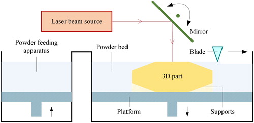
Existing AM processes were divided into seven categories, where powder bed fusion is one of them (ISO 17296-2 2015). In this process, either a laser beam or an electron beam is used to fuse the powder material together to fabricate a 3D part (Shuai et al. 2019; Wang et al. 2020a, 2020b). According to the energy source, powder bed fusion can be further classified into selective laser sintering, electron beam melting, direct metal laser melting and selective laser melting, where the latter two processes are commonly referred to as laser powder bed fusion (LPBF) (Yap, Chua, and Dong 2016; Sing and Yeong 2020). An LPBF machine, whose schematic diagram is depicted in Figure 1, generally consists of a build platform, a powder bed, a recoater blade, a powder feeding apparatus, a laser beam source and a moving mirror. The use of an LPBF machine to build a 3D part includes the following steps:

(1)	A layer of powder material from the powder feeding apparatus is spread on the build platform by the recoater blade;
(2)	A moving laser beam generated by the laser beam source and the moving mirror is applied to selectively fuse the powder material to create a layer of the part;
(3)	The build platform is lowered and a new layer of powder material from the powder feeding apparatus is spread over its previous layer by the recoater blade;
(4)	The second and third steps are repeated until the entire part is completely formed.

LPBF allows rapid fabrication of parts with relatively high mechanical performance directly from powders without the time-consuming mould design process (Yu et al. 2019a, 2019b). This makes it an attractive technology for producing high-quality functional components in aerospace, automotive and biomedical industries (Huang et al. 2020; Sing and Yeong 2020).

Figure 1. Schematic diagram of the LPBF process.

Generally, the application of the LPBF process to realise a product consists of five activities, where process planning is an indispensable one (Kim et al. 2015; Qin et al. 2020a). Process planning for LPBF is the planning of the process parameters to build a part using an LPBF machine, which mainly include the build orientation, supports, slices, laser scanning path and machine parameters (Ahsan, Habib, and Khoda 2015). It includes four preparation tasks before the fabrication of a part (Kulkarni, Marsan, and Dutta 2000). Part orientation is the first task, which directly affects its three subsequent tasks: support generation, model slicing and path planning (Du et al. 2018; Jiang, Xu, and Stringer 2018, 2019a, 2019b; Zhao and Guo 2020; Jiang and Ma 2020).

In the LPBF process, the orientation to build a part is one of the most essential process parameters, since it has an important influence on the time and cost to build the part and the quality and properties of the as-built part (Edwards and Ramulu 2014; Wauthle et al. 2015; Calignano 2018; Li et al. 2018; Kuo et al. 2020; Du et al. 2020). Part orientation for LPBF is the determination of an optimal orientation to build a part using an LPBF machine based on certain production requirements on the part. In real workshops, an LPBF machine operator usually determines the build orientation of an LPBF part according to their production experience and intuitive analysis on the part. Different operators could determine different build orientations for an identical part under the same production requirements. This would have a negative influence on the quality and properties of the part.

In this paper, a method for automatic determination of part build orientation for LPBF is proposed. This method determines the build orientation of an LPBF part based on a two-step strategy. First, a facet clustering-based approach presented by Qin et al. (2020b) is applied to automatically generate the alternative orientations of the part. Second, an optimal orientation to build the part is selected via a multi-objective decision-making process, in which the objectives are to simultaneously optimise the support volume, volumetric error, surface roughness, build time and build cost.

The remainder of the paper is organised as follows: Section 2 documents an overview of related work. Section 3 explains the details of the proposed method. Section 4 reports the demonstration of the method. Section 5 ends the paper with a conclusion together with a suggestion of some future research directions.

2. Related work

The main research topics involved in automatic determination of part build orientation for LPBF include design for AM, process planning for AM, and part orientation for AM. In this section, a brief introduction of the first and second topics is, respectively, provided. Then a review of the the existing research work on the third topic is presented. Based on the review, the importance of the proposed method is clarified.

2.1. Design for AM

Design for AM refers to an activity of designing an AM product, in which the functional performance and other key lifecycle considerations such as manufacturability, reliability and cost of the product are optimised subjected to the capabilities of the used AM process (Rosen 2014a, 2014b; Rosen et al. 2015; Thompson et al. 2016; Vaneker et al. 2020). The design mainly includes two tasks, which are conceptual design and detailed design. Conceptual design is the very first stage of AM product realisation process, in which the outline of function and the form of an AM product are articulated. It involves the design of interactions, experiences, processes and strategies and serves to provide a description of the proposed AM product in terms of concept sketches (Williams, Mistree, and Rosen 2011).

Detailed design is the stage where the design is refined and the plans, specifications and estimates are created. The most important task in this stage is geometry design (Gao et al. 2015). In general, geometry design for AM is carried out via either computer-aided design (CAD) modelling or reverse engineering. CAD modelling is performed in a CAD system based on the result of conceptual design and outputs a tessellated 3D model of the product, which is generally encoded in STL (standard tessellation language), OBJ (Wavefront object), 3MF (3D manufacturing format) or AMF (additive manufacturing file) format (Qin et al. 2019b). Reverse engineering generates a tessellated 3D model of a 3D object from its 2D image or physical model. The tessellated 3D model is also encoded in a specific format like STL, OBJ, 3MF or AMF.

In addition to geometry design, detailed design also involves the design of specifications of an AM product and the selection of an AM machine to fabricate the product (Qin et al. 2020a). Generally, the specifications to be designed can be classified from macro, micro and production levels. Macro level specifications mainly include tolerance, topology, material, colour and properties. Surface texture, material composition and porosity are three major micro level specifications. An important production level specification is cost models for AM production. The details about the design of these specifications can be found from the studies of Thompson et al. (2016) and Vaneker et al. (2020).

2.2. Process planning for AM

In traditional subtractive manufacturing, process planning generally involves determination of machining processes and corresponding parameters for converting a workpiece from an engineering drawing to the final form. In AM, the engineering drawing and machining processes are respectively replaced by tessellated 3D model and AM processes. The aim of process planning remains the same, namely, to determine specific AM process plans to enable efficient and accurate manufacture of a part (Newman et al. 2015). Process planning for AM includes four successive tasks, which are part orientation, support generation, model slicing and path planning (Kulkarni, Marsan, and Dutta 2000). In real AM workshops, these tasks are completed in software tools supplied by AM machine manufacturers. However, the four tasks are common for all AM processes. Effective methods can be developed to carry out in an integrated process planning system outside AM machines.

Part orientation is required for all AM processes. It aims to determine a desirable orientation to build a part via carrying out a comprehensive analysis of a tessellated 3D model of the part and specific production requirements and preferences on the part (Di Angelo, Di Stefano, and Guardiani 2020). In this task, the tessellated 3D model is the output from the AM design activity. The production requirements and preferences are specified by AM designers or AM process planners.

Support generation is required for the AM processes that are not free of supports (e.g. material jetting, electron beam melting, LPBF). It aims to determine the minimum supports needed for building a part through performing a geometric analysis of a tessellated 3D model of the part in a specified orientation (Jiang, Xu, and Stringer 2018). In this task, the tessellated 3D model in a specified orientation is the output of the part orientation task.

Model slicing transforms process planning from 3D model domain to layer domain. It is needed for all AM processes. The slicing task involves intersecting a 3D model with a horizontal plane. Its input is a tessellated 3D model of a part with supports in a specified orientation, and its output includes the thickness of individual layers and the geometry of the contour to be accumulated. In general, the output information is encoded in a proprietary file format. Apart from the tessellated 3D model, slicing can also be carried out on an original CAD model or a reverse engineering model (Zhao and Guo 2020).

Path planning is a pure layer domain task and is also required for all AM processes. It aims to determine the tool path and process parameters for building each layer from slices of a tessellated 3D model of a part. Path planning can be divided into inner path planning and outer path planning. Inner path planning mainly addresses determination of the pattern and geometric coordinates of the inner path and the associated process parameters. Outer path planning controls the accuracy of the outer boundary of a slice. It involves the use of a material-removing tool to form the outer boundary of a slice to a 3D shape (Zhao and Guo 2020).

2.3. Part orientation for AM

To implement the automation of part orientation for AM, there are many available methods in the literature (Di Angelo, Di Stefano, and Guardiani 2020). These methods can be categorised into one-step methods and two-step methods on the basis of the process they solve the part orientation issue. Theoretically, a 3D part has an infinite number of possible build orientations. A one-step method generally develops a specialised algorithm (Alexander, Allen, and Dutta 1998; Delfs, Tows, and Schmid 2016; Golmohammadi and Khodaygan 2019; Griffiths et al. 2019; Ulu et al. 2020; Wang and Qian 2020) or applies an existing optimisation algorithm, such as the genetic algorithm (Hur et al. 2001; Masood, Rattanawong, and Iovenitti 2003; Thrimurthulu, Pandey, and Reddy 2004; Ahn, Kim, and Lee 2007; Padhye and Deb 2011; Zhang and Li 2013; Paul and Anand 2015; Brika et al. 2017; Chowdhury, Mhapsekar, and Anand 2018), particle swarm algorithm (Padhye and Deb 2011; Cheng and To 2019; Raju et al. 2019; Shen et al. 2020) or bacterial foraging algorithm (Raju et al. 2019), to directly search an orientation enabling one or more part orientation factors to be optimal from infinite possible orientations. In a one-step method, the 3D model of a part is first rotated with a random or fixed angle. Then certain estimation models of the considered part orientation factors are used to estimate the values of the factors under each rotation (which corresponds to an orientation to be evaluated). An optimal orientation is produced by an multi-objective optimisation procedure, in which the objective function value under each rotation is a summary value of the considered factors under this rotation. There is usually a contradictory issue in this process: How to set a suitable iteration number or rotation angle? If the iteration number or rotation angle is set too large, the number of computation of the objective function values can be reduced, but the risk of missing the true optimal orientation will be very high; If it is set too small, such risk can be reduced, but it will greatly increase the number of computation. For this reason, most of the existing one-step methods suffer from the issue of high computational cost, which make them difficult to be applied to part orientation in real workshops.

A two-step method divides the part orientation task into two successive steps. The first step is to generate a small number of alternative orientations from infinite possible orientations. In the existing two-step methods, such generation is realised by reference plane searching (Lan et al. 1997), convex hull detection (Xu, Loh, and Wong 1999; West, Sambu, and Rosen 2001; Byun and Lee 2006), shape feature recognition (Zhang et al. 2016; Al-Ahmari, Abdulhameed, and Khan 2018; Qin et al. 2019a) and facet clustering (Zhang et al. 2019; Qin et al. 2020b). The second step is to select an optimal orientation from the generated alternatives. The selection is generally completed by a multi-objective decision-making process (West, Sambu, and Rosen 2001; Byun and Lee 2006; Zhang et al. 2016; Qin et al. 2019a). In this process, certain estimation models of the considered part orientation factors are first used to estimate the values of the factors under each alternative. Then a summary value of the considered factors under each alternative is calculated using an aggregation model. An optimal orientation is selected based on the calculated summary values. From such principle, it can be seen that a two-step method focuses on a small number of alternatives. It will not spend time on a large number of meaningless orientations like a one-step method. However, the methods based on reference plane searching or shape feature recognition are not realistic for freeform surface models, because such models do not have reference plane and it is difficult to define suitable shape features for them. The methods based on convex hull detection have an accuracy issue, since convex hull is not the exact 3D model. Compared to these methods, the method based on facet clustering of Zhang et al. (2019) can avoid reference plane searching and shape feature recognition, and most importantly work for both regular and freeform surface models. But this method could produce unstable and unreasonable results and would not be efficient for a high-resolution 3D model. The method based on facet clustering of Qin et al. (2020b) provides a practical tool for automatic generation of alternative orientations for LPBF. This method maintains the advantages of the method of Zhang et al. (2019) and can overcome its limitations, but the method does not address the selection of an optimal orientation from the generated alternatives.

2.4. Importance of the proposed method

In this paper, the line of research in Qin et al. (2020b) is continued and a complete method for rapid determination of part build orientation for LPBF is proposed. This method adopts the two-step strategy to determine the build orientation of an LPBF part. The first step is completed using the method of Qin et al. (2020b), while the second step is realised by an automatic selection approach based on multi-objective decision-making. Compared to the existing one-step methods, the proposed method can provide desired efficiency, since it does not need to spend time on a large number of meaningless orientations. Compared to the existing two-step methods based on reference plane searching, convex hull detection and shape feature recognition, the proposed method does not have the accuracy issue and are applicable for both regular and freeform surface models. Compared to the existing two-step method based on facet clustering, the proposed method can produce stable and reasonable results and simultaneously provide higher efficiency.

3. Details of the proposed method

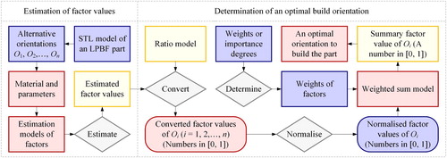
In this section, a method for automatic determination of the build orientation of an LPBF part is presented. The schematic representation of this method is depicted in Figure 2. As can be seen from the figure, the presented method takes as input the 3D model of an LPBF part encoded in the STL format, together with the material, layer thickness, recoating time, hatch spacing and scanning velocity to build the part and the weights or importance degrees of the considered part orientation factors support volume, volumetric error, surface roughness, build time and build cost. It outputs an optimal orientation to build the part, together with the estimated factor values of the part in this orientation. This method consists of an alternative orientation generation step and an optimal orientation selection step. In the former step, a small number of alternative orientations of an LPBF part are automatically generated by the method of Qin et al. (2020b). The objective of the latter step is to select an orientation from the generated alternatives that can simultaneously optimise the considered factors. To achieve this, an automatic selection approach based on multi-objective decision-making is developed, whose working process is shown in Figure 3. Firstly, certain estimation models are applied to estimate the values of the considered factors in each alternative orientation. Then each estimated factor value is converted into a number in [0, 1] using a ratio model and the converted results are normalised. After that, the weights of the considered factors are either directly input or determined. Finally, a summary value of the factors in each alternative orientation is calculated by the weighted sum model, and an optimal orientation is generated according to the calculated summary values.

Figure 2. Framework of the proposed build orientation determination method.

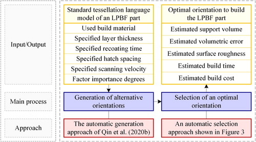
Figure 3. Schematic diagram of an optimal orientation selection approach.

For the details regarding the alternative orientation generation step, please refer to (Qin et al. 2020b). The present section explains the details of the optimal orientation selection step, which consists of estimation of factor values and determination of an optimal orientation.

3.1. Factor value estimation

According to the studies of Edwards and Ramulu (2014), Wauthle et al. (2015), Brika et al. (2017), Cheng and To (2019) and Griffiths et al. (2019), the build orientation factors (i.e. the factors affected by the build orientation) of an LPBF part include support volume, volumetric error, surface roughness, build time, build cost, strength, elongation, hardness, residual stress, fatigue performance, distortion and microstructure. Among them, the support volume, volumetric error, surface roughness, build time and build cost in a given build orientation can be estimated via analysing the geometry of the STL model of the part:

(1) Support volume. When the angle between the normal vector of a planar triangular facet of the STL model of an LPBF part and the build orientation is greater than a threshold (commonly 135 deg), this facet is considered as an overhang and additional supports are required to sustain the overhang to avoid collapse or build failure during the fabrication of the part. Apart from overhangs, supports are also needed for the top areas of a hollow 3D model. In process planning for LPBF, the total volume of the supports required for a part is an important factor, because it has direct influence on the build time and build cost of the part. To estimate the total support volume of an LPBF part, Autodesk Meshmixer, a free software for working with triangle meshes, is applied in the proposed method. Firstly, the STL model of an LPBF part is imported into the software. Then the model is rotated around the x axis by an angle of ${\theta }_{\mathrm{x}}$ and rotated around the y axis by an angle of ${\theta }_{\mathrm{y}}$, so that the build orientation O given by a unitised vector (x, y, z) is vertically upward. After the rotations, supports can be generated and their volume (${\mathrm{m}\mathrm{m}}^3$) can be estimated by the software. In this process, the angles (deg) ${\theta }_{\mathrm{x}}$ and ${\theta }_{\mathrm{y}}$ can be obtained via the following equations (Zhang et al. 2019): (1) ${\theta }_{\mathrm{x}}=\left\{\begin{array}{cc}\arctan \left(y/z\right)& \mathrm{i}\mathrm{f}y\ne 0\mathrm{o}\mathrm{r}z\ne 0\\ 0& \mathrm{i}\mathrm{f}y=0\mathrm{a}\mathrm{n}\mathrm{d}z=0\end{array}\right.$(1) (2) ${\theta }_{\mathrm{y}}=-\arctan \frac{x}{\sqrt{y^2+z^2}}$(2) In theory, the greater the total support volume, the longer the build time, and the higher the build cost. The objective is to minimise the total support volume if it is one of the part orientation factors considered in the optimal orientation determination.

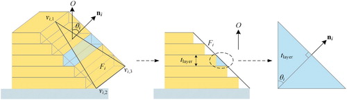
(2) Volumetric error. There are two types of surface errors in LPBF. The first type appears in the tessellation of 3D models. It is caused by approximating a surface with a set of planar triangles and can be reduced via controlling the chordal error. The second type is the so-called volumetric error, which is caused by fabricating each facet with staircases in a layer upon layer manner and may have significant influence on the shape accuracy of the as-built parts. Volumetric error cannot be eliminated, but its effect can be reduced via specifying appropriate build orientation and layer thickness. To date, a number of models for estimating the total volumetric error of an AM part have been presented. Representative examples are the estimation models in Masood, Rattanawong, and Iovenitti (2003), Zhang and Li (2013), and Luo and Wang (2016). In the proposed method, the model in Luo and Wang (2016) is used to estimate the total volumetric error of an LPBF part in a given build orientation O. Firstly, the volumetric error of each facet in the STL model of an LPBF part in O is estimated via geometric analysis. The total volumetric error of the part in O is then obtained by calculating the sum of the volumetric error of all facets. Suppose the STL model of an LPBF part includes $n^{\prime }$ facets $F_1=(v_{1,1},v_{1,2},v_{1,3})$, $F_2=(v_{2,1},v_{2,2},v_{2,3})$,…, $F_{n^{\mathrm{\prime }}}=(v_{n^{\prime },1},v_{n^{\prime },2},v_{n^{\prime },3})$. Then the total volumetric error (${\mathrm{m}\mathrm{m}}^3$) of this part in O, as illustrated in Figure 4, can be estimated using the following equation: (3) $E_{\mathrm{v}\mathrm{o}\mathrm{l}\mathrm{u}\mathrm{m}\mathrm{e}\mathrm{t}\mathrm{r}\mathrm{i}\mathrm{c}}^O=\sum _{i=1}^{n^{\prime }}{E}_i=\sum _{i=1}^{n^{\prime }}(\frac{1}{2}{t}_{\mathrm{l}\mathrm{a}\mathrm{y}\mathrm{e}\mathrm{r}}|\cos {\theta }_i|A_i)$(3) where $E_i$ is the volumetric error (${\mathrm{m}\mathrm{m}}^3$) of $F_i$, $t_{\mathrm{L}\mathrm{a}\mathrm{y}\mathrm{e}\mathrm{r}}$ is the layer thickness (mm) in O, ${\theta }_i$ is the angle (deg) between the normal vector of $F_i$ and O, and $A_i$ is the area (${\mathrm{m}\mathrm{m}}^2$) of $F_i$ that can be calculated using the following equation: (4) $A_i=\sqrt{p_i(p_i-d(v_{i,1},v_{i,2}))(p_i-d(v_{i,1},v_{i,3}))(p_i-d(v_{i,2},v_{i,3}))}$(4) where $d(v_{i,1},v_{i,2})$, $d(v_{i,1},v_{i,3})$ and $d(v_{i,2},v_{i,3})$ are, respectively, the lengths (mm) of the three edges of $F_i$ and (5) $p_i=\frac{1}{2}(d(v_{i,1},v_{i,2})+d(v_{i,1},v_{i,3})+d(v_{i,2},v_{i,3}))$(5) Generally, the greater the total volumetric error of an LPBF part, the greater the impact on the shape accuracy of the part. Thus, the objective is to minimise the total volumetric error if it is one of the part orientation factors considered in the optimal orientation determination.

Figure 4. An illustration of the volumetric error of a facet.

(3) Surface roughness. Surface roughness reflects the unevenness of a real surface. It is generally quantified by the deviations in the normal vector direction of the real surface from its ideal form. Small deviations indicate that the real surface is smooth. There are a number of different parameters available for describing surface roughness (ISO 4287 1997), where Ra is the most common by far. In the field of AM, Ra is also the most commonly used parameter for measuring the surface roughness of an AM part (Strano et al. 2013; Calignano 2018). Without loss of generality, Ra will also be used to quantify the surface roughness of an LPBF part in this paper. In the literature, many estimation models of the average surface roughness of an AM part are established based on the staircase effect caused by the layer upon layer building manner of AM processes. However, according to the research findings of Strano et al. (2013) and Calignano (2018), the estimation models based on staircase effect cannot accurately predict the average surface roughness of an LPBF part, since it is mainly affected by build orientation and process parameters. In the method of Brika et al. (2017), a model for estimating the average surface roughness of an LPBF part was established on the basis of a study of the average surface roughness of LPBF Ti6Al4V samples in different build orientations and with a constant layer thickness of 0.03 mm. This model is used to predict the average surface roughness of an LPBF part in a given build orientation O in the proposed method. Firstly, the surface roughness of each facet in the STL model of an LPBF part in O is estimated by a linear regression function. Then the roughness per unit area is calculated and used as the average surface roughness of the part in O. Suppose the STL model of an LPBF part includes $n^{\prime }$ facets $F_1=(v_{1,1},v_{1,2},v_{1,3})$, $F_2=(v_{2,1},v_{2,2},v_{2,3})$,…, $F_{n^{\mathrm{\prime }}}=(v_{n^{\prime },1},v_{n^{\prime },2},v_{n^{\prime },3})$. The average surface roughness (mm) of this part in O can be estimated using the following equation: (6) $R{a}^O=\frac{\sum _{i=1}^{n^{\prime }}\left(R{a}_i{A}_i\right)}{\sum _{i=1}^{n^{\prime }}{A}_i}=\frac{\sum _{i=1}^{n^{\prime }}((0.0094148+0.0000389|{\theta }_i-90\left|\right)A_i)}{\sum _{i=1}^{n^{\prime }}{A}_i}$(6) where $R{a}_i$ is the surface roughness (mm) of $F_i$ in O, $A_i$ is the area (${\mathrm{m}\mathrm{m}}^2$) of $F_i$ that can be calculated using Equation (4(4) $A_i=\sqrt{p_i(p_i-d(v_{i,1},v_{i,2}))(p_i-d(v_{i,1},v_{i,3}))(p_i-d(v_{i,2},v_{i,3}))}$(4) ), and ${\theta }_i$ is value of the angle (deg) between the normal vector of $F_i$ and O. For an as-built LPBF part, the greater the average surface roughness, the worse the surface quality. Therefore, the objective is to minimise the average surface roughness if it is one of the part orientation factors considered in the optimal orientation determination.

(4) Build time. Build time and build cost are two important indicators for nearly all AM processes. Many of the existing part orientation methods consider these factors and establish their estimation models with respect to build orientation and process parameters under specific AM processes. To estimate the build time of an LPBF part in a given build orientation O, an estimation model for LPBF process presented by Brika et al. (2017) is introduced. According to the model, the total build time (s) of an LPBF part in O can be estimated using the following equation: (7) $T_{\mathrm{b}\mathrm{u}\mathrm{i}\mathrm{l}\mathrm{d}}^O=\frac{h_{\mathrm{m}\mathrm{o}\mathrm{d}\mathrm{e}\mathrm{l}}^O}{t_{\mathrm{l}\mathrm{a}\mathrm{y}\mathrm{e}\mathrm{r}}}{T}_{\mathrm{r}\mathrm{e}\mathrm{c}\mathrm{o}\mathrm{a}\mathrm{t}\mathrm{i}\mathrm{n}\mathrm{g}}+\frac{V_{\mathrm{m}\mathrm{o}\mathrm{d}\mathrm{e}\mathrm{l}}+V_{\mathrm{s}\mathrm{u}\mathrm{p}\mathrm{p}\mathrm{o}\mathrm{r}\mathrm{t}}^O}{R_{\mathrm{b}\mathrm{u}\mathrm{i}\mathrm{l}\mathrm{d}}}$(7) where $R_{\mathrm{b}\mathrm{u}\mathrm{i}\mathrm{l}\mathrm{d}}$ is the build rate (${\mathrm{m}\mathrm{m}}^3$/s), i.e. the volume deposited per unit time, and other symbols are explained in Table 1. The build rate can be calculated using the following equation (Tang, Pistorius, and Beuth 2017): (8) $R_{\mathrm{b}\mathrm{u}\mathrm{i}\mathrm{l}\mathrm{d}}=t_{\mathrm{l}\mathrm{a}\mathrm{y}\mathrm{e}\mathrm{r}}{s}_{\mathrm{h}\mathrm{a}\mathrm{t}\mathrm{c}\mathrm{h}}{v}_{\mathrm{s}\mathrm{c}\mathrm{a}\mathrm{n}\mathrm{n}\mathrm{i}\mathrm{n}\mathrm{g}}$(8) where all symbols are also defined in Table 1. Obviously, the objective is to minimise the total build time if it is one of the part orientation factors considered in the optimal orientation determination.

Table 1. An explanation of the symbols in the estimation model of build time.

Symbol	Meaning	Unit	Value
$h_{\mathrm{m}\mathrm{o}\mathrm{d}\mathrm{e}\mathrm{l}}^O$	STL model height in O	mm	Calculate according to the STL model and O
$t_{\mathrm{l}\mathrm{a}\mathrm{y}\mathrm{e}\mathrm{r}}$	Layer thickness	mm	Specify based on the technical data of the used machine
$T_{\mathrm{r}\mathrm{e}\mathrm{c}\mathrm{o}\mathrm{a}\mathrm{t}\mathrm{i}\mathrm{n}\mathrm{g}}$	Recoating time	s	Specify based on the technical data of the used machine
$V_{\mathrm{m}\mathrm{o}\mathrm{d}\mathrm{e}\mathrm{l}}$	STL model volume	${\mathrm{m}\mathrm{m}}^3$	Calculate according to the STL model
$V_{\mathrm{s}\mathrm{u}\mathrm{p}\mathrm{p}\mathrm{o}\mathrm{r}\mathrm{t}}^O$	Support volume in O	${\mathrm{m}\mathrm{m}}^3$	Estimate using the Autodesk Meshmixer software
$s_{\mathrm{h}\mathrm{a}\mathrm{t}\mathrm{c}\mathrm{h}}$	Hatch spacing	mm	Specify based on the technical data of the used machine
$v_{\mathrm{s}\mathrm{c}\mathrm{a}\mathrm{n}\mathrm{n}\mathrm{i}\mathrm{n}\mathrm{g}}$	Laser scanning velocity	mm/s	Specify based on the technical data of the used machine

(5) Build cost. To estimate the build cost of an LPBF part in a given build orientation, a generic estimation model presented by Baumers et al. (2016) is used. According to the model, build cost consists of direct cost and indirect cost, where the direct cost includes material cost and energy cost. That is, the total build cost (GBP) of an LPBF part in a given build orientation O is the sum of the material cost, energy cost and indirect cost of the part in O. This can be described by the following equation: (9) $C_{\mathrm{b}\mathrm{u}\mathrm{i}\mathrm{l}\mathrm{d}}^O=C_{\mathrm{m}\mathrm{a}\mathrm{t}\mathrm{e}\mathrm{r}\mathrm{i}\mathrm{a}\mathrm{l}}^O+C_{\mathrm{e}\mathrm{n}\mathrm{e}\mathrm{r}\mathrm{g}\mathrm{y}}^O+C_{\mathrm{i}\mathrm{n}\mathrm{d}\mathrm{i}\mathrm{r}\mathrm{e}\mathrm{c}\mathrm{t}}^O$(9) According to a build cost estimation model for LPBF process proposed by Brika et al. (2017), the material cost (GBP), energy cost (GBP) and indirect cost (GBP) in O can be respectively calculated using the following equations: (10) $\begin{array}{rl}{C}_{\mathrm{m}\mathrm{a}\mathrm{t}\mathrm{e}\mathrm{r}\mathrm{i}\mathrm{a}\mathrm{l}}^O=& (V_{\mathrm{m}\mathrm{o}\mathrm{d}\mathrm{e}\mathrm{l}}+V_{\mathrm{s}\mathrm{u}\mathrm{p}\mathrm{p}\mathrm{o}\mathrm{r}\mathrm{t}}^O)\\ & (1+r_{\mathrm{w}\mathrm{a}\mathrm{s}\mathrm{t}\mathrm{e}}){\rho }_{\mathrm{m}\mathrm{a}\mathrm{t}\mathrm{e}\mathrm{r}\mathrm{i}\mathrm{a}\mathrm{l}}{P}_{\mathrm{m}\mathrm{a}\mathrm{t}\mathrm{e}\mathrm{r}\mathrm{i}\mathrm{a}\mathrm{l}}{p}_{\mathrm{m}\mathrm{a}\mathrm{t}\mathrm{e}\mathrm{r}\mathrm{i}\mathrm{a}\mathrm{l}}\end{array}$(10) (11) $\begin{array}{rl}{C}_{\mathrm{e}\mathrm{n}\mathrm{e}\mathrm{r}\mathrm{g}\mathrm{y}}^O=& (V_{\mathrm{m}\mathrm{o}\mathrm{d}\mathrm{e}\mathrm{l}}+V_{\mathrm{s}\mathrm{u}\mathrm{p}\mathrm{p}\mathrm{o}\mathrm{r}\mathrm{t}}^O)\\ & {\rho }_{\mathrm{m}\mathrm{a}\mathrm{t}\mathrm{e}\mathrm{r}\mathrm{i}\mathrm{a}\mathrm{l}}{P}_{\mathrm{m}\mathrm{a}\mathrm{t}\mathrm{e}\mathrm{r}\mathrm{i}\mathrm{a}\mathrm{l}}{R}_{\mathrm{k}\mathrm{W}\mathrm{h}/\mathrm{k}\mathrm{g}}{p}_{\mathrm{e}\mathrm{n}\mathrm{e}\mathrm{r}\mathrm{g}\mathrm{y}}\end{array}$(11) (12) $C_{\mathrm{i}\mathrm{n}\mathrm{d}\mathrm{i}\mathrm{r}\mathrm{e}\mathrm{c}\mathrm{t}}^O=R_{\mathrm{G}\mathrm{B}\mathrm{P}/\mathrm{h}}{T}_{\mathrm{b}\mathrm{u}\mathrm{i}\mathrm{l}\mathrm{d}}^O$(12) where all symbols are explained in Table 2. Obviously, the objective is to minimise the total build cost if it is one of the part orientation factors considered in the optimal orientation determination.

Table 2. An explanation of the symbols in the estimation model of build cost.

Symbol	Meaning	Unit	Value
$V_{\mathrm{m}\mathrm{o}\mathrm{d}\mathrm{e}\mathrm{l}}$	STL model volume	${\mathrm{m}}^3$	Calculate according to the STL model
$V_{\mathrm{s}\mathrm{u}\mathrm{p}\mathrm{p}\mathrm{o}\mathrm{r}\mathrm{t}}^O$	Support volume in O	${\mathrm{m}}^3$	Estimate using the Autodesk Meshmixer software
$r_{\mathrm{w}\mathrm{a}\mathrm{s}\mathrm{t}\mathrm{e}}$	Material waste ratio	–	0.1, found from the data used in Ruffo, Tuck, and Hague (2006)
${\rho }_{\mathrm{m}\mathrm{a}\mathrm{t}\mathrm{e}\mathrm{r}\mathrm{i}\mathrm{a}\mathrm{l}}$	Density of material	$\mathrm{k}\mathrm{g}/{\mathrm{m}}^3$	Find from the technical data of the used material
$P_{\mathrm{m}\mathrm{a}\mathrm{t}\mathrm{e}\mathrm{r}\mathrm{i}\mathrm{a}\mathrm{l}}$	Porosity of material	–	Find from the technical data of the used material
$p_{\mathrm{m}\mathrm{a}\mathrm{t}\mathrm{e}\mathrm{r}\mathrm{i}\mathrm{a}\mathrm{l}}$	Price of material	GBP/kg	Find from the material supplier's website
$R_{\mathrm{k}\mathrm{W}\mathrm{h}/\mathrm{k}\mathrm{g}}$	Consumption rate	kWh/kg	162.13, found from the data used in Brika et al. (2017)
$p_{\mathrm{e}\mathrm{n}\mathrm{e}\mathrm{r}\mathrm{g}\mathrm{y}}$	Price of energy	GBP/kWh	Find from the energy supplier's website
$R_{\mathrm{G}\mathrm{B}\mathrm{P}/\mathrm{h}}$	Indirect cost rate	GBP/h	44.08, converted from 53.35 USD/h in Brika et al. (2017)
$T_{\mathrm{b}\mathrm{u}\mathrm{i}\mathrm{l}\mathrm{d}}^O$	Build time in O	h	Calculate using the estimation model in Equation (7(7) $T_{\mathrm{b}\mathrm{u}\mathrm{i}\mathrm{l}\mathrm{d}}^O=\frac{h_{\mathrm{m}\mathrm{o}\mathrm{d}\mathrm{e}\mathrm{l}}^O}{t_{\mathrm{l}\mathrm{a}\mathrm{y}\mathrm{e}\mathrm{r}}}{T}_{\mathrm{r}\mathrm{e}\mathrm{c}\mathrm{o}\mathrm{a}\mathrm{t}\mathrm{i}\mathrm{n}\mathrm{g}}+\frac{V_{\mathrm{m}\mathrm{o}\mathrm{d}\mathrm{e}\mathrm{l}}+V_{\mathrm{s}\mathrm{u}\mathrm{p}\mathrm{p}\mathrm{o}\mathrm{r}\mathrm{t}}^O}{R_{\mathrm{b}\mathrm{u}\mathrm{i}\mathrm{l}\mathrm{d}}}$(7) )

Compared to the support volume, volumetric error, surface roughness, build time and build cost, the strength, elongation, hardness, residual stress, fatigue performance, distortion and microstructure of an LPBF part in a given build orientation are more difficult to estimate. Although several existing part orientation methods, such as the methods of Zhang et al. (2016), Brika et al. (2017), Cheng and To (2019) and Raju et al. (2019), have considered some of these factors, the estimation models in them are either not for the LPBF process or incomplete. From other existing literature, such as the articles of Bartolomeu et al. (2016), Mukherjee, Zhang, and DebRoy (2017), Vastola, Pei, and Zhang (2018), Li et al. (2019) and Tan, Sing, and Yeong (2020), some related estimation models can be found. However, build orientation is not a variable in these models. To this end, the estimation of the strength, elongation, hardness, residual stress, fatigue performance, distortion and microstructure of an LPBF part in a given build orientation is not considered in the proposed method for the time being.

3.2. Optimal orientation determination

The basic components of an optimal orientation selection problem in the proposed method include a set of alternative orientations $\mathbf{O}=\{O_1,O_2,\dots ,O_m\}$, a set of part orientation factors $\mathbf{F}=\{F_1,F_2,\dots ,F_n\}$, a vector of weights of part orientation factors $\mathbf{w}=[w_1,w_2,\dots ,w_n{]}^{\mathrm{T}}$ and a decision matrix $\mathbf{M}=[v_{i,j}{]}_{m\times n}$, where $O_1,O_2,\dots ,O_m$ are m alternative orientations of an LPBF part generated by the method of Qin et al. (2020b), $F_1,F_2,\dots ,F_n$ are n different part orientation factors considered in optimal orientation determination, $v_{i,j}$ is the value of the j-th factor of the i-th alternative orientation, and $w_1,w_2,\dots ,w_n$ are respectively the weights of $F_1,F_2,\dots ,F_n$ such that $0\le w_1,w_2,\dots ,w_n\le 1$ and $w_1+w_2+\cdots +w_n=1$. Based on these components, the optimal orientation determination for an LPBF part is carried out according to the following steps:

(1) Convert each estimated factor value of the part into a number in [0, 1]. To make the estimated factor values easy to process, each of them is converted into a number in [0, 1]. A ratio model can be used to implement such conversion. Brauers et al. (2008) tested a set of ratio models and found that the best ratio model for transforming real numbers into the numbers in [0, 1] is: (13) ${\alpha }_{i,j}=\frac{v_{i,j}}{\sqrt{\sum _{i=1}^m{v}_{i,j}^2}}$(13) This model is used to convert the estimated factor values into the numbers in [0, 1] in the proposed method. That is, the decision matrix M is converted into a matrix ${\mathbf{M}}_{\mathrm{C}}=[{\alpha }_{i,j}{]}_{m\times n}$ using the ratio model.

(2) Normalise the converted results. In general, there are two different types of factors in a multi-objective decision-making problem, i.e. positive and negative factors. Positive factors have positive effect on the decision-making result, while negative factors affect the result adversely. For example, tensile strength and surface roughness, respectively, belong to positive and negative factors in optimal orientation determination for an LPBF part, since they, respectively, have positive and negative influences on the determination result. To unify the effect of different types of factors on the decision-making result, a complement rule is usually adopted to normalise the numbers quantifying the values of negative factors. This rule is also used to normalise the converted factor values in the proposed method. 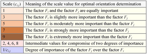That is, the converted decision matrix ${\mathbf{M}}_C$ is normalised as ${\mathbf{M}}_N=[x_{i,j}{]}_{m\times n}$, where (14) $x_{i,j}=\left\{\begin{array}{cc}{\alpha }_{i,j}& \text{ if {F\_j} is a positive factor}\\ 1-{\alpha }_{i,j}& \text{ if {F\_j} is a negative factor}\end{array}\right.$(14) (3) Determine the weights of the considered factors. In the proposed method, the weights of the considered factors are used to measure their relative importance for optimal orientation determination. The values of factor weights are either directly assigned by users or determined via pairwise comparison. If a user directly provides the values of the weights of factors, this step will be skipped. If a user explicitly specifies the importance degrees of each pair of factors for optimal orientation determination, the weight values will be calculated using a scaling approach based on pairwise comparison (Saaty 1977). This approach determines the weight vector $\mathbf{w}=[w_1,w_2,\dots ,w_n{]}^{\mathrm{T}}$ from a positive reciprocal pairwise comparison matrix $\mathbf{C}=[c_{i,j}{]}_{n\times n}$, where $c_{i,j}$ is the scale value which stands for the degree of importance of the factor $F_i$ over the factor $F_j$ for optimal orientation determination and are defined in Figure 5.

Figure 5. Definition of the elements of a pairwise comparison matrix.

According to the positive reciprocity, all $c_{i,j}$ must satisfy the conditions that $c_{i,j}>0$ and $c_{i,j}=1/c_{j,i}$. The matrix $\mathbf{C}$ is consistent if and only if $c_{i,k}{c}_{k,j}=c_{i,j}$ for all $i,j,k=1,2,\dots ,n$. In practical applications, the matrix is not necessarily consistent. But the inconsistencies must be controlled within a certain range. To define the range of inconsistencies, three indicators named consistency index (CI), random index (RI) and consistency ratio (CR) were introduced. The value of CI can be calculated via the following equation: (15) $CI=\frac{{\lambda }_{\mathrm{m}\mathrm{a}\mathrm{x}}-n}{n-1}$(15) where ${\lambda }_{\mathrm{m}\mathrm{a}\mathrm{x}}$ is the maximum eigenvalue of the matrix $\mathbf{C}$. RI is the average consistency rate of 500 randomly constructed n-order pairwise comparison matrices ${\mathbf{C}}_1,{\mathbf{C}}_2,\dots ,{\mathbf{C}}_{500}$, whose value can be computed using the following equation: (16) $RI=\frac{\sum _{i=1}^{500}C{I}_i}{500}$(16) where $C{I}_1,C{I}_2,\dots ,C{I}_{500}$ are the CI values of the matrices ${\mathbf{C}}_1,{\mathbf{C}}_2,\dots ,{\mathbf{C}}_{500}$, respectively. The values of RI from n=1 to n=15 are listed in Table 3.

Table 3. The random index values when the matrix order is within 15.

n	1	2	3	4	5	6	7	8	9	10	11	12	13	14	15
RI	0.00	0.00	0.58	0.90	1.12	1.24	1.32	1.41	1.45	1.49	1.51	1.54	1.56	1.57	1.59

CR is defined as the ratio of CI and RI: (17) $CR=\frac{CI}{RI}$(17) If the CR value of a pairwise comparison matrix $\mathbf{C}$ is negative, then $\mathbf{C}$ is not a positive reciprocal matrix and the elements of $\mathbf{C}$ need to be adjusted until all $c_{i,j}$ satisfy the conditions that $c_{i,j}>0$ and $c_{i,j}=1/c_{j,i}$. If CR=0, then $\mathbf{C}$ is a consistent matrix. If 0<CR<0.10, then the inconsistencies in $\mathbf{C}$ are acceptable. When $\mathbf{C}$ is consistent or its inconsistencies are acceptable, the normalised principal eigenvector is used as the weight vector $\mathbf{w}$. That is, the normalised ${\mathbf{w}}^{\prime }(\mathbf{C}{\mathbf{w}}^{\prime }={\lambda }_{\mathrm{m}\mathrm{a}\mathrm{x}}{\mathbf{w}}^{\prime })$ is used as $\mathbf{w}$. Otherwise, the inconsistent scale values in the matrix $\mathbf{C}$ need to be adjusted until $0\le CR<0.10$. To sum up, the determination of factor weights using the scaling approach based on pairwise comparison includes three steps. The first step is to construct a positive reciprocal pairwise comparison matrix $\mathbf{C}$ according to Figure 5. The second step is to calculate the CR value of the matrix $\mathbf{C}$ using Equation (17(17) $CR=\frac{CI}{RI}$(17) ). In the last step, the factor weights are determined as the elements of the normalised principal eigenvector of the matrix $\mathbf{C}$ if $0\le CR<0.10$. Otherwise, the inconsistent scale values in the matrix $\mathbf{C}$ are adjusted and the second step is repeated until $0\le CR<0.10$. For example, suppose the degrees of importance of the factors support volume, volumetric error, surface roughness, build time and build cost for optimal orientation determination are expressed in the following positive reciprocal pairwise comparison matrix: $\mathbf{C}=\left[\begin{array}{ccccc}1& 3& 3& 1/2& 1/2\\ 1/3& 1& 1& 1/4& 1/4\\ 1/3& 1& 1& 1/2& 1/2\\ 2& 4& 2& 1& 1/5\\ 2& 4& 2& 5& 1\end{array}\right]$

The maximum eigenvalue of this matrix is ${\lambda }_{\mathrm{m}\mathrm{a}\mathrm{x}}=5.4899$. According to Equation (17(17) $CR=\frac{CI}{RI}$(17) ), the CR value of the matrix $\mathbf{C}$ is 0.1094. Since CR>0.10, the inconsistencies in $\mathbf{C}$ are unacceptable. If the scale values $c_{4,5}$ and $c_{5,4}$ in $\mathbf{C}$ are, respectively, adjusted to 1/2 and 2, that is, the degrees of importance of the five factors are expressed by the following matrix: $\mathbf{C}=\left[\begin{array}{ccccc}1& 3& 3& 1/2& 1/2\\ 1/3& 1& 1& 1/4& 1/4\\ 1/3& 1& 1& 1/2& 1/2\\ 2& 4& 2& 1& 1/2\\ 2& 4& 2& 2& 1\end{array}\right]$ then ${\lambda }_{\mathrm{m}\mathrm{a}\mathrm{x}}=5.2097$ and CR=0.0468. Since $0<CR<0.10$, the inconsistencies are acceptable. The principal eigenvector of $\mathbf{C}$ is ${\mathbf{w}}^{\prime }=[0.4095,0.1561,0.2147,0.5275,0.6954{]}^{\mathrm{T}}$. By normalising ${\mathbf{w}}^{\prime }$, the factor weight vector is $\mathbf{w}=[0.2044,0.0779,0.1072,0.2633,0.3472{]}^{\mathrm{T}}$.

(4) Calculate a summary value of factors in each alternative orientation. Part orientation problem is a typical multi-objective problem. A general solution for such problem is to transform it into a single-objective problem, because a decision can be made easier under a single-objective function value than multiple objective function values (Di Angelo, Di Stefano, and Guardiani 2020). In the existing part orientation methods (Lan et al. 1997; Hur et al. 2001; Thrimurthulu, Pandey, and Reddy 2004; Byun and Lee 2006; Paul and Anand 2015; Brika et al. 2017; Chowdhury, Mhapsekar, and Anand 2018), one of the most efficient and widely used model to achieve such transformation is the weighted sum model. This model is used to calculate a summary value of the factors in each alternative orientation in the proposed method. That is, the summary value of factors in the alternative orientation $O_i(i=1,2,\dots ,m)$ is calculated using the following equation: (18) $f\left(O_i\right)=f(x_{i,1},x_{i,2},\dots ,x_{i,n})=\sum _{j=1}^n(w_j{x}_{i,j})$(18) where $x_{i,j}$ are the elements of the normalised decision matrix ${\mathbf{M}}_{\mathrm{N}}$ and $w_j$ is the determined weight of the factor $F_j$.

(5) Generate an optimal orientation for the part. Each of the alternative orientations having the maximum summary value of factors is generated as an optimal orientation for the part.

4. Demonstration of the proposed method

In this section, a set of examples are first presented to illustrate the application of the proposed method. Then theoretical analysis and comparisons to the existing part orientation methods are carried out to evaluate the method.

4.1. Case studies

Twelve parts are used as cases to illustrate the application of the proposed method. The STL models of these parts are shown in Figure 6. The basic information of the parts is listed in Table 4. Among all STL models in Figure 6, the STL model of Part 4 was provided by Zhang et al. (2016). The STL models of the remaining parts were downloaded from Thingiverse, a free and open-source online community for sharing 3D models. Based on the surface types, the 12 STL models can be divided into two groups. The first group includes the STL models from Part 1 to Part 6, which are all regular surface models. The STL models from Part 7 to Part 12 constitute the second group, as all of them belong to freeform surface models. The reasons for choosing these models can be roughly explained from two aspects. On the one hand, the number of the facets in the twelve models increases sequentially. This will facilitate the subsequent efficiency comparison, since the part orientation time and the number of facets are positively correlated. On the other hand, the twelve models include six regular surface models and six freeform surface models, which will demonstrate that the proposed method is applicable for both types of models.

Figure 6. The STL models of 12 LPBF parts.

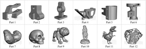
Table 4. The basic information of the 12 LPBF parts.

Part Unit	Vertices –	Facets –	Surface –	Length mm	Width mm	Height mm	Area ${\mathrm{m}\mathrm{m}}^2$	Volume ${\mathrm{m}\mathrm{m}}^3$
Part 1	140	284	Regular	38.31	10.00	25.40	2629.50	2864.45
Part 2	410	828	Regular	27.00	16.00	23.00	2535.94	4593.24
Part 3	798	1592	Regular	120.00	80.00	167.89	60,941.50	404,405.00
Part 4	1181	2426	Regular	74.09	33.75	34.34	9137.33	9603.15
Part 5	1876	3776	Regular	125.00	75.00	80.00	46,576.40	228,889.00
Part 6	3160	6324	Regular	160.00	122.00	162.00	96,711.40	639,850.00
Part 7	6610	13,240	Freeform	35.89	26.48	22.04	2408.50	7354.99
Part 8	33,863	67,722	Freeform	119.81	88.13	94.90	36,451.00	535,216.00
Part 9	44,368	88,724	Freeform	86.06	56.88	68.00	17,165.80	88,637.20
Part 10	51,216	104,352	Freeform	34.05	33.88	60.00	5172.53	908.27
Part 11	54,314	108,888	Freeform	132.16	58.46	125.00	23,930.60	120,669.00
Part 12	80,276	161,606	Freeform	48.32	40.93	40.00	6915.89	1914.96

Suppose the 12 parts will be built using Ti6Al4V and the LPBF machine EOSINT M270. The values of layer thickness, recoating time, hatch spacing, laser scanning velocity, material density, material porosity and material price are cited from (Brika et al. 2017) and listed in Table 5. The value of energy price is obtained from the energy supplier's website and also provided in Table 5. Before building the parts, the four preparation tasks, part orientation, support generation, model slicing and path planning, are needed to be completed in sequence. The present paper focuses on part orientation using the proposed method. It is further assumed that support volume, volumetric error, surface roughness, build time and build cost are the factors considered in the determination of an optimal build orientation of each part and the importance degrees of these factors are specified in the following positive reciprocal pairwise comparison matrix: $\mathbf{C}=\left[\begin{array}{ccccc}1& 2& 2& 1& 1\\ 1/2& 1& 2& 1/2& 1/2\\ 1/2& 1/2& 1& 1/3& 1/3\\ 1& 2& 3& 1& 1\\ 1& 2& 3& 1& 1\end{array}\right]$

Table 5. The values of some variables for estimating factor values.

Variable Unit	$t_{\mathrm{l}\mathrm{a}\mathrm{y}\mathrm{e}\mathrm{r}}$ mm	$T_{\mathrm{r}\mathrm{e}\mathrm{c}\mathrm{o}\mathrm{a}\mathrm{t}\mathrm{i}\mathrm{n}\mathrm{g}}$ s	$s_{\mathrm{h}\mathrm{a}\mathrm{t}\mathrm{c}\mathrm{h}}$ mm	$v_{\mathrm{s}\mathrm{c}\mathrm{a}\mathrm{n}\mathrm{n}\mathrm{i}\mathrm{n}\mathrm{g}}$ mm/s	${\rho }_{\mathrm{m}\mathrm{a}\mathrm{t}\mathrm{e}\mathrm{r}\mathrm{i}\mathrm{a}\mathrm{l}}$ kg/${\mathrm{m}}^3$	$P_{\mathrm{m}\mathrm{a}\mathrm{t}\mathrm{e}\mathrm{r}\mathrm{i}\mathrm{a}\mathrm{l}}$ –	$p_{\mathrm{m}\mathrm{a}\mathrm{t}\mathrm{e}\mathrm{r}\mathrm{i}\mathrm{a}\mathrm{l}}$ GBP/kg	$p_{\mathrm{e}\mathrm{n}\mathrm{e}\mathrm{r}\mathrm{g}\mathrm{y}}$ GBP/kWh
Value	0.03	20	0.07	1,250	4,430	99.5%	247.86	0.16

Based on the conditions above, the build orientation for each of the twelve parts can be automatically determined using the proposed method. For example, the build orientation of Part 1 is determined via the following steps:

(1) Generate the alternative orientations for building the part. The alternative orientations of the part are automatically generated by the method of Qin et al. (2020b). It is worth noting that the number of facet clusters used to generate alternative orientations is set as 6 for regular surface models and is set as 12 for freeform surface models when using the method. The generated alternative orientations are listed in the first column of Table 6. The schematic diagram of these alternative orientations is shown in Figure 7.

Figure 7. Schematic diagram of the generated alternative orientations of Part 1.

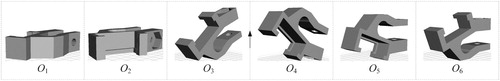
Table 6. The estimated factor values in the alternative orientations of Part 1.

Generated alternative orientation	$V_{\mathrm{s}\mathrm{u}\mathrm{p}\mathrm{p}\mathrm{o}\mathrm{r}\mathrm{t}}^{O_i}$	$E_{\mathrm{v}\mathrm{o}\mathrm{l}\mathrm{u}\mathrm{m}\mathrm{e}\mathrm{t}\mathrm{r}\mathrm{i}\mathrm{c}}^{O_i}$	$R{a}^{O_i}$	$T_{\mathrm{b}\mathrm{u}\mathrm{i}\mathrm{l}\mathrm{d}}^{O_i}$	$C_{\mathrm{b}\mathrm{u}\mathrm{i}\mathrm{l}\mathrm{d}}^{O_i}$
Unit of the factor value	${\mathrm{m}\mathrm{m}}^3$	${\mathrm{m}\mathrm{m}}^3$	μm	h	GBP
$O_1=(+0.0000,+0.0000,-1.0000)$	218.6600	22.1375	10.4642	2.1781	100.0687
$O_2=(+0.0000,+0.0000,+1.0000)$	145.9500	22.1375	10.4642	2.1704	99.6339
$O_3=(-0.3420,-0.9397,+0.0000)$	1880.5100	24.8010	10.9248	5.6166	253.8252
$O_4=(+0.3420,+0.9397,+0.0000)$	2610.2700	23.8270	10.9248	5.6938	258.1897
$O_5=(+0.0000,+1.0000,+0.0000)$	2408.1200	25.0293	10.9584	5.0262	228.4960
$O_6=(+0.0000,-1.0000,+0.0000)$	1731.7600	25.2946	10.9584	4.9547	224.4509

(2) Estimate the values of the considered factors in each alternative orientation. Using the estimation models from Equation (1(1) ${\theta }_{\mathrm{x}}=\left\{\begin{array}{cc}\arctan \left(y/z\right)& \mathrm{i}\mathrm{f}y\ne 0\mathrm{o}\mathrm{r}z\ne 0\\ 0& \mathrm{i}\mathrm{f}y=0\mathrm{a}\mathrm{n}\mathrm{d}z=0\end{array}\right.$(1) ) to Equation (12(12) $C_{\mathrm{i}\mathrm{n}\mathrm{d}\mathrm{i}\mathrm{r}\mathrm{e}\mathrm{c}\mathrm{t}}^O=R_{\mathrm{G}\mathrm{B}\mathrm{P}/\mathrm{h}}{T}_{\mathrm{b}\mathrm{u}\mathrm{i}\mathrm{l}\mathrm{d}}^O$(12) ), the values of the five factors in each generated alternative orientation of Part 1 are estimated. The estimated results are listed in Table 6.

(3) Convert each estimated factor value of the part into a number in [0, 1]. The estimated values of the five factors in each generated alternative orientation of Part 1 are converted into the numbers in [0, 1] using the ratio model in Equation (13(13) ${\alpha }_{i,j}=\frac{v_{i,j}}{\sqrt{\sum _{i=1}^m{v}_{i,j}^2}}$(13) ). A converted decision matrix is obtained as follows: ${\mathbf{M}}_{\mathrm{C}}=\left[\begin{array}{ccccc}0.0499& 0.3780& 0.3961& 0.1962& 0.1987\\ 0.0333& 0.3780& 0.3961& 0.1955& 0.1978\\ 0.4290& 0.4235& 0.4135& 0.5060& 0.5040\\ 0.5954& 0.4069& 0.4135& 0.5129& 0.5127\\ 0.5493& 0.4274& 0.4148& 0.4528& 0.4537\\ 0.3950& 0.4319& 0.4148& 0.4463& 0.4457\end{array}\right]$

(4) Normalise the converted results. For each of the five factors, the objective is to minimise the value of the factor. Thus, each of them is a negative factor. According to Equation (14(14) $x_{i,j}=\left\{\begin{array}{cc}{\alpha }_{i,j}& \text{ if {F\_j} is a positive factor}\\ 1-{\alpha }_{i,j}& \text{ if {F\_j} is a negative factor}\end{array}\right.$(14) ), the converted decision matrix ${\mathbf{M}}_{\mathrm{C}}$ is normalised as follows: ${\mathbf{M}}_{\mathrm{N}}=\left[\begin{array}{ccccc}0.9501& 0.6220& 0.6039& 0.8038& 0.8013\\ 0.9667& 0.6220& 0.6039& 0.8045& 0.8022\\ 0.5710& 0.5765& 0.5865& 0.4940& 0.4960\\ 0.4046& 0.5931& 0.5865& 0.4871& 0.4873\\ 0.4507& 0.5726& 0.5852& 0.5472& 0.5463\\ 0.6050& 0.5681& 0.5852& 0.5537& 0.5543\end{array}\right]$

(5) Determine the weights of the considered factors. The weights of the considered factors are calculated by the scaling approach based on pairwise comparison. The maximum eigenvalue of the pairwise comparison matrix $\mathbf{C}$ is ${\lambda }_{\mathrm{m}\mathrm{a}\mathrm{x}}=5.0394$. According to Equation (17(17) $CR=\frac{CI}{RI}$(17) ), the CR value of $\mathbf{C}$ is $CR=0.0088$. Since 0<CR<0.10, the inconsistencies in $\mathbf{C}$ are acceptable. The principal eigenvector of $\mathbf{C}$ is ${\mathbf{w}}^{\prime }=[0.5148,0.2954,0.1915,0.5528,0.5528{]}^{\mathrm{T}}$. By normalising ${\mathbf{w}}^{\prime }$, the factor weight vector is $\mathbf{w}=[0.2443,0.1402,0.0909,0.2623,0.2623{]}^{\mathrm{T}}$.

(6) Calculate a summary value of factors in each alternative orientation. Using Equation (18(18) $f\left(O_i\right)=f(x_{i,1},x_{i,2},\dots ,x_{i,n})=\sum _{j=1}^n(w_j{x}_{i,j})$(18) ), the summary values of the five factors in the six alternative orientations of Part 1 are calculated as follows:

$f\left(O_1\right)=0.7952$; $f\left(O_2\right)=0.7997$; $f\left(O_3\right)=0.5333$; $f\left(O_4\right)=0.4909$; $f\left(O_5\right)=0.5304$; $f\left(O_6\right)=0.5712$

(7) Generate an optimal orientation for the part. Since $O_2$ is the only alternative orientation that has the maximum summary value of factors, it is generated as the optimal orientation for Part 1. The schematic diagram of this orientation is shown in Figure 8. The estimated factor values of the part in this orientation are listed in Table 7.

Figure 8. The generated optimal orientation of each of the 12 LPBF parts.

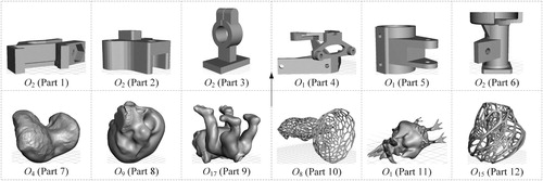
Table 7. The estimated factor values in the optimal orientation of each of the 12 LPBF parts.

Part	Generated optimal orientation	$V_{\mathrm{s}\mathrm{u}\mathrm{p}\mathrm{p}\mathrm{o}\mathrm{r}\mathrm{t}}^{O_i}$	$E_{\mathrm{v}\mathrm{o}\mathrm{l}\mathrm{u}\mathrm{m}\mathrm{e}\mathrm{t}\mathrm{r}\mathrm{i}\mathrm{c}}^{O_i}$	$R{a}^{O_i}$	$T_{\mathrm{b}\mathrm{u}\mathrm{i}\mathrm{l}\mathrm{d}}^{O_i}$	$C_{\mathrm{b}\mathrm{u}\mathrm{i}\mathrm{l}\mathrm{d}}^{O_i}$
–	Unit of the factor value	${\mathrm{m}\mathrm{m}}^3$	${\mathrm{m}\mathrm{m}}^3$	μm	h	GBP
Part 1	$O_2=(+0.0000,+0.0000,+1.0000)$	145.9500	22.1375	10.4642	2.1704	99.6339
Part 2	$O_2=(+1.0000,+0.0000,+0.0000)$	167.4100	21.4108	10.5592	3.4667	159.0793
Part 3	$O_2=(+0.0000,+0.0000,+1.0000)$	13,377.0000	551.7687	10.8011	75.3003	3,869.0913
Part 4	$O_1=(+0.0000,+1.0000,+0.0000)$	4587.1500	78.8480	10.6058	7.7516	360.3676
Part 5	$O_1=(+0.0000,+0.0000,-1.0000)$	13,022.0000	375.1246	10.2877	40.4139	2,099.8284
Part 6	$O_2=(+0.0000,+0.0000,-1.0000)$	39,032.0000	840.0294	10.6613	101.8394	5,382.5733
Part 7	$O_4=(-0.0007,+0.0001,+0.9999)$	1183.3700	22.8656	10.6987	4.9844	230.9516
Part 8	$O_9=(-0.9746,+0.1419,+0.1731)$	15,849.0000	347.5876	10.8183	79.2603	4,219.0663
Part 9	$O_{17}=(+0.0884,+0.1803,+0.9796)$	10,913.8000	164.3367	10.6973	23.2229	1,154.6889
Part 10	$O_8=(+0.1199,-0.9915,+0.0500)$	8317.5850	49.3868	10.6976	7.2288	330.7878
Part 11	$O_1=(+0.9802,-0.1916,-0.0503)$	24,248.0000	228.8950	10.9073	26.9175	1,377.2533
Part 12	$O_{15}=(+0.4968,+0.2169,+0.8403)$	10,813.0400	66.2267	10.8418	8.4612	389.7227

For each of the remaining 11 parts, the build orientation can be determined via the same steps. The results of alternative orientation generation for the eleven parts are provided in Figures S1–S11. The results of factor value estimation for the eleven parts are listed in Tables S1–S11. The results of optimal orientation determination for the 12 parts are listed in Table 7 and depicted in Figure 8.

4.2. Effectiveness analysis

The main components of the proposed method are the alternative orientation generation approach in Qin et al. (2020b) and the optimal orientation selection approach in Section 2. An effectiveness analysis is carried out via, respectively, analysing the effectiveness of these two approaches.

In general, whether a build orientation determination method is effective depends on whether the determined build orientations can meet the pre-set objective. The objective of the proposed method is to concurrently optimise the total support volume, total volumetric error, average surface roughness, total build time and total build cost. It has been demonstrated in Qin et al. (2020b) that the alternative orientation generation approach can theoretically benefit the simultaneous optimisation of the total support volume, average surface roughness, total build time and total build cost of an LPBF part.

The optimal orientation selection approach applies the weighted sum model to determine a build orientation which can simultaneously optimise the total support volume, total volumetric error, average surface roughness, total build time and total build cost from the alternative orientations generated by the alternative orientation generation approach. From this principle, it is not difficult to conclude that the proposed method is theoretically effective.

4.3. Efficiency comparison

Theoretically, the time complexity of the alternative orientation generation approach of Qin et al. (2020b) is $O\left(n^{\prime }\mathrm{l}\mathrm{o}\mathrm{g}{n}^{\prime }\right)$, where $n^{\prime }$ is the number of facets of an STL model. The used estimation models of volumetric error, surface roughness, build time and build cost on m alternative orientations and $n^{\prime }$ facets have $O\left(m{n}^{\prime }\right)$ run-time. The optimal orientation determination on m alternative orientations and n factors has $O\left(mn\right)$ run-time. Therefore, the time complexity of the proposed method is $O(n^{\prime }\mathrm{l}\mathrm{o}\mathrm{g}{n}^{\prime }+m{n}^{\prime }+mn)$.

From the theoretical analysis above, it is difficult to imagine how efficient the proposed method is. To this end, an efficiency testing experiment and two efficiency comparison experiments were carried out on a machine with Intel(R) Core(TM) i9-7900X CPU, 8 GB RAM and NVIDIA GeForce GTX 1080 Ti GPU:

(1) Experiment 1. The purpose of this experiment is to test the time spent on determination of the build orientations of specific LPBF parts for the proposed method. In the experiment, the STL models of the twelve parts in Figure 6 were taken as input of the proposed method. For each STL model, the method was executed ten times. The results of the experiment are the average time spent on alternative orientation generation, factor value estimation and optimal orientation determination for the method, which are listed in Table 8. It is worth noting that the time of factor value estimation does not include the time spent on estimation of support volume, because this estimation was completed by Autodesk Meshmixer and it is very difficult to count the exact time spent on the estimation of this software. The average time of the entire part orientation process of the proposed method is the sum of the average time of alternative orientation generation, factor value estimation and optimal orientation determination, which is also listed in Table 8. As can be concluded from the table, most of the build orientation determination time is spent on factor value estimation for each part. The proposed method can generate the optimal orientation of a regular surface model within several seconds. It is also efficient for a freeform surface model.

Table 8. The actual build orientation determination time of the proposed method.

The input STL model of LPBF part (.stl)	Part 1	Part 2	Part 3	Part 4	Part 5	Part 6
Number of facets in the STL model ($n^{\prime }$)	284	828	1592	2426	3776	6324
Number of the alternative orientations (m)	6	6	6	8	8	8
Time of alternative orientation generation (s)	0.0156	0.0625	0.1106	0.1597	0.2895	0.4538
Time of factor value estimation (s)	0.0984	0.2681	0.5140	1.0292	1.5887	2.6461
Time of optimal orientation determination (s)	0.0150	0.0150	0.0147	0.0156	0.0156	0.0156
Time of the entire part orientation process (s)	0.1290	0.3456	0.6393	1.2045	1.8938	3.1155
The input STL model of LPBF part (.stl)	Part 7	Part 8	Part 9	Part 10	Part 11	Part 12
Number of facets in the STL model ($n^{\prime }$)	13,240	67,722	88,724	104,352	108,888	161,606
Number of the alternative orientations (m)	24	24	24	24	24	24
Time of alternative orientation generation (s)	0.9607	5.9256	9.6683	10.2501	10.6240	18.1546
Time of factor value estimation (s)	16.5983	84.8202	110.7432	131.0347	135.5582	202.8251
Time of optimal orientation determination (s)	0.0315	0.0310	0.0312	0.0313	0.0315	0.0313
Time of the entire part orientation process (s)	17.5905	90.7768	120.4427	141.3161	146.2137	221.0110

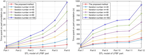
(2) Experiment 2. The purpose of this experiment is to compare the build orientation determination time taken by an existing one-step method and the proposed method with respect to specific STL models. As reviewed in Section 1, there are many one-step methods in the literature. It is not realistic to implement each method and compare its execution time with that of the proposed method on specific STL models. However, it is still possible to compare the build orientation determination time of an existing one-step method and the proposed method with respect to specific STL models, because factor value estimation is an indispensable task for each method and most of the build orientation determination time is spent on this task (see Table 8). The time of factor value estimation is determined by the number of iterations (alternative orientations) for a one-step method (the proposed method) and the number of factors. It is found from experiments that the effect of the number of iterations (alternative orientations) on the time of factor value estimation is roughly uniform. If it is assumed that the effect of the number of alternative orientations on the time of alternative orientation generation and the time of optimal orientation determination in Table 8 is also roughly uniform, the time of the entire part orientation process per alternative orientation calculated from the data in the table can be used to estimate the time of the entire part orientation process of an existing one-step method. Take Part 1 as an example, as the time of the entire part orientation process for the STL model is 0.1290 s and the number of the alternative orientations is 6, the time of the entire part orientation process per alternative orientation for the STL model is 0.1290/6 s. Suppose an existing one-step method needs to perform computation on 20 iterations. The time of the entire part orientation process of this method for the STL model of Part 1 is $20\times 0.1290/6\mathrm{s}=0.4300$  s. By this way, the time of the entire part orientation process of an existing one-step method for the STL models of the twelve parts in Figure 6 when the number of iterations m=20, 40, 60, 80, 100 is estimated. Based on the estimated results, a comparison of the part orientation time of an existing one-step method and the proposed method with respect to the 12 STL models is depicted in Figure 9. It can be concluded from the figure that an existing one-step method could outperform the proposed method when m is smaller than the number of the generated alternative orientations for the STL model of each part. However, most of the existing one-step methods are difficult to generate optimal solutions in such few iterations. For instance, an optimisation algorithm for optimising AM process parameters generally requires 100 iterations to obtain the optimal solutions according to the study of Raju et al. (2019). From this point of view, the proposed method has obvious advantage in efficiency over a one-step method.

Figure 9. Efficiency comparison result of the proposed method and an existing one-step method.

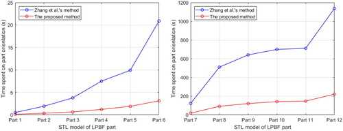
(3) Experiment 3. The purpose of this experiment is to compare the build orientation determination time taken by the facet clustering-based method of Zhang et al. (2019) and the proposed method with respect to specific STL models. In the experiment, the STL models of Part 1 to Part 12 in Figure 6 were respectively taken as the input of the two methods. Each of these methods was executed 10 times for each STL model. The value of k in Zhang et al.'s method was assigned 6 for Part 1 to Part 6 and assigned 12 for Part 7 to Part 12. Further, it is assumed that the time of factor value estimation and the time of optimal orientation determination of the two methods are the same for each part to ensure the fairness of the comparison. The result of the experiment is the average time spent on part orientation of the two methods, which is depicted in Figure 10. As can be seen from the figure, the proposed method consumes significantly less time than Zhang et al.'s method consumes for the STL models of every part. This shows that the proposed method has higher efficiency than Zhang et al.'s method.

Figure 10. Efficiency comparison result of the proposed method and Zhang et al.'s method.

4.4. Characteristic comparison

Section 1 classified the existing part orientation methods into one-step methods and two-step methods, where two steps methods were further divided into reference plane searching based methods, convex hull detection based methods, shape feature recognition based methods and facet clustering based methods. It also described the main characteristics of these methods. Briefly, the one-step methods can be applied to both regular and freeform surface models, but they generally need expensive computation to obtain desired results. The reference plane searching based methods and the shape feature recognition based methods can greatly reduce the amount of computation, but they are not applicable for freeform surface models. The convex hull detection based methods have an accuracy issue. The facet clustering based method of Zhang et al. (2019) can address the limitations of these three types of two-step methods, but it suffers from the issues of producing unstable and unreasonable results and having relatively low efficiency.

Compared to the existing one-step methods, the proposed method does not need to spend time on the computation of meaningless build orientations. This has been demonstrated in Experiment 2 in Section 3.3. Compared to the existing reference plane searching based methods and shape feature recognition based methods, the proposed method is applicable for both regular and freeform surface models. This has been illustrated in Section 3.1. Compared to the facet clustering based method of Zhang et al. (2019), the proposed method has the advantages in generating stable and reasonable results and providing higher efficiency. The first advantage was verified in Qin et al. (2020b). The second advantage has been demonstrated in Experiment 3 in Section 3.3.

5. Conclusion

In this paper, an automatic determination method of part build orientation for LPBF has been proposed. This method includes a step of alternative orientation generation and a step of optimal orientation selection. In the former step, the approach of Qin et al. (2020b) is applied to automatically generate the alternative orientations of an LPBF part. In the latter step, the part orientation factors support volume, volumetric error, surface roughness, build time and build cost are considered and the values of these factors in each alternative orientation are estimated using certain estimation models. The estimated factor values are converted into the numbers in [0, 1] by a ratio model and the converted results are normalised via a normalisation rule. A scaling approach based on pairwise comparison is introduced to determine the weights of the considered factors. With the normalised factor values and determined factor weights, the weighted sum model is used to calculate a summary value of the factors in each alternative orientation. An optimal orientation of the part is generated according to the calculated results. The paper has also presented a set of part orientation cases to illustrate the application of the proposed method and evaluated the method via effectiveness analysis and efficiency and characteristic comparisons. The evaluation results suggest that the proposed method is theoretically effective and can be applied to both regular and freeform surface models. Further, the results also show that the method can produce stable and reasonable results and provide desired efficiency.

Detailed work in the present paper revealed several limitations of the proposed method, which need to be addressed in future work:

(1)	Build orientation determination for multi-part production in LPBF. An important characteristic of the LPBF process is the support of multi-part production. The proposed method focuses on build orientation determination for production of one single part, it is not applicable for the situation where a group of parts in the same build need to be orientated simultaneously. It is of necessity and importance to improve the method to deal with this situation.
(2)	Improvement of the proposed method to consider the mechanical properties of the as-built parts. The LPBF process results in anisotropic mechanical properties. Desired mechanical properties may sometimes be more important than support volume, volumetric error, surface roughness, build time and build cost, as they are of importance for the quality of an as-built part. The proposed method does not consider the mechanical properties of the as-built parts because of the availability of suitable estimation models. It will be extended to take into account these factors once suitable estimation models are available.
(3)	Systematic determination of the process parameters to build an LPBF part. In LPBF, the influence of process parameters on part quality and production stability is comprehensive and contradictory. As one example, varying build orientations will result in different laser scanning patterns in slices. Different types of scanning patterns may contribute to deviations for the part quality. As another example, success in layer upon layer bonding in LPBF are quite dependent on recoating time and slice areal properties. Delamination may occur if these process parameters are not taken into well consideration. The proposed method studies the build orientation determination issue separately by fixing other process parameters, which is sometimes insufficient. An ideal way is to comprehensively determine all process parameters via weighing certain part quality factors. To this end, it would be desirable to extend the proposed method to implement the systematic determination of the process parameters to build an LPBF part.
(4)	Integration of the proposed method into CAD systems. The proposed method is a stand-alone method for automatically determining the build orientation of an LPBF part. The ultimate goal of the research of part orientation for LPBF is to integrate novel methods into CAD systems to assist design and process planning for LPBF. To this end, it would be desirable to study and implement the integration of the proposed method into CAD systems.

Acknowledgments

The authors are very grateful to the five anonymous reviewers for their insightful comments for the improvement of the paper. The authors are also very grateful to Dr Yicha Zhang at the Department of Mechanical Engineering and Design, University of Technology of Belfort-Montbéliard, France for providing the STL file of Part 4.

Disclosure statement

No potential conflict of interest was reported by the author(s).

Data availability

The STL files of the 12 LPBF parts and the implementation code of the proposed method have been deposited in the GitHub repository (https://github.com/YuchuChingQin/LPBFPartOrientation).

Additional information

Funding

This work was supported by the EPSRC UKRI Innovation Fellowship [grant number EP/S001328/1], the EPSRC Fellowship in Manufacturing [grant number EP/R024162/1], and the EPSRC Future Advanced Metrology Hub [grant number EP/P006930/1].

Notes on contributors

Yuchu Qin

Yuchu Qin is currently a PhD candidate and a part-time research fellow at the EPSRC Future Advanced Metrology Hub, University of Huddersfield, UK. He received a PhD degree in Measurement Technology and Instrument from School of Mechanical Science and Engineering, Huazhong University of Science and Technology, China in 2017. He has an MSc degree in Computer Application Technology and a BSc degree in Computer Science and Technology. His research interests include Intelligent Manufacturing, Computational Intelligence, and Knowledge Engineering. He has published over thirty papers about these research topics in a number of international journals such as Virtual and Physical Prototyping, Robotics and Computer-Integrated Manufacturing, Knowledge-Based Systems, Journal of Intelligent Manufacturing, Computers & Industrial Engineering, Computer-Aided Design, and Advanced Engineering Informatics.

Qunfen Qi

Qunfen Qi is currently a senior research fellow at the EPSRC Future Advanced Metrology Hub, University of Huddersfield, UK. She received a Ph.D. degree in Precision Engineering from University of Huddersfield in 2013. She is an EPSRC UKRI Innovation Fellow, an EPSRC Peer Review Full College Member, an EPSRC Women in Engineering Society (WES) member, and a fellow of the Higher Education Academy (FHEA). Her research lies in knowledge modelling for manufacturing covering smart information systems, abstract mathematical theory (category theory), geometrical product specifications and verification (GPS), additive manufacturing (AM), and surface metrology. She has worked for fifteen years in developing decision-making tools for smart product design and inspection, using category theory as its foundation.

Peizhi Shi

Peizhi Shi is currently a research fellow at the EPSRC Future Advanced Metrology Hub, University of Huddersfield, UK. He received a PhD degree in Computer Science from School of Computer Science, the University of Manchester, UK in 2019, a Master's degree in Software Engineering from the University of Science and Technology of China in 2013, and a BSc degree in Computer Science and Technology from Guilin University of Electronic Technology, China in 2010. His current research interests include machine learning, active learning, 3D object classification, machine perception, and their applications in manufacturing domain.

Paul J. Scott

Paul J. Scott is currently a professor at the EPSRC Future Advanced Metrology Hub of the University of Huddersfield. He received a Ph.D. degree in Statistics from Imperial College London in 1983. He has an honours degree in Mathematics and an M.Sc. degree in Statistics. His research interests are in manufacturing informatics, geometrical product specifications and verification, philosophy of the measurement of product geometry, and foundations of specifying and characterising solutions for real world industrial problems. He was the project leader for twenty published ISO standards and is currently working on four new ISO documents. He is a fellow of Royal Statistical Society (FRSS), an EPSRC fellow of Manufacturing, a leading member of ISO TC 213, a founder member of the strategic group AG1 and the technical review group AG2 of ISO TC 213, a convenor of the working group WG15 and the advisory group AG12 of ISO TC 213, a core member of BSI TDW4, a convenor of BSI TDW4/-/9, a visiting industrial professor of Taylor Hobson Ltd., and the Taylor Hobson Chair for Computational Geometry.

Xiangqian Jiang

Xiangqian Jiang is currently the chair professor and the director of the EPSRC Future Advanced Metrology Hub, University of Huddersfield and the Royal Academy of Engineering and Renishaw Chair in Precision Metrology. She has a D.Sc. degree in Precision Engineering and a Ph.D. degree in Surface Metrology. Her research interests mainly lie in Surface Measurement, Precision Engineering, and Advanced Manufacturing Technologies. She was made a Dame Commander of the Order of the British Empire for services to Engineering and Manufacturing in 2017. She is a fellow of the Royal Academy of Engineering (FREng), a fellow of the Royal Society of Arts (FRSA), a fellow of the Institute of Engineering Technologies (FIET), a fellow of the International Academy of Production Research (FCIRP), a fellow of the International Society for Nanomanufacturing (FISNM), a principle member of ISO TC 213 and BSI TW/4, an advisory member for UK national measurement system, and the UK Chairman of the International Academy of Production Research.

References

- Ahn, D., H. Kim, and S. Lee. 2007. “Fabrication Direction Optimization to Minimize Post-Machining in Layered Manufacturing.” International Journal of Machine Tools and Manufacture 47 (3-4): 593–606.
- Ahsan, A. N., M. A. Habib, and B. Khoda. 2015. “Resource Based Process Planning for Additive Manufacturing.” Computer-Aided Design 69: 112–125.
- Al-Ahmari, A. M., O. Abdulhameed, and A. A. Khan. 2018. “An Automatic and Optimal Selection of Parts Orientation in Additive Manufacturing.” Rapid Prototyping Journal 24 (4): 698–708.
- Alexander, P., S. Allen, and D. Dutta. 1998. “Part Orientation and Build Cost Determination in Layered Manufacturing.” Computer-Aided Design 30 (5): 343–356.
- Bartolomeu, F., S. Faria, O. Carvalho, E. Pinto, N. Alves, F. S. Silva, and G. Miranda. 2016. “Predictive Models for Physical and Mechanical Properties of Ti6Al4V Produced by Selective Laser Melting.” Materials Science and Engineering: A 663: 181–192.
- Baumers, M., P. Dickens, C. Tuck, and R. Hague. 2016. “The Cost of Additive Manufacturing: Machine Productivity, Economies of Scale and Technology-push.” Technological Forecasting and Social Change 102: 193–201.
- Brauers, W. K. M., E. K. Zavadskas, F. Peldschus, and Z. Turskis. 2008. “Multi-Objective Decision-making for Road Design.” Transport 23 (3): 183–193.
- Brika, S. E., Y. F. Zhao, M. Brochu, and J. Mezzetta. 2017. “Multi-Objective Build Orientation Optimisation for Powder Bed Fusion by Laser.” Journal of Manufacturing Science and Engineering 139 (11): 111011.
- Byun, H.-S., and K. H. Lee. 2006. “Determination of the Optimal Build Direction for Different Rapid Prototyping Processes Using Multi-criterion Decision Making.” Robotics and Computer-Integrated Manufacturing 22 (1): 69–80.
- Calignano, F.. 2018. “Investigation of the Accuracy and Roughness in the Laser Powder Bed Fusion Process.” Virtual and Physical Prototyping 13 (2): 97–104.
- Cheng, L., and A. To. 2019. “Part-scale Build Orientation Optimization for Minimizing Residual Stress and Support Volume for Metal Additive Manufacturing: Theory and Experimental Validation.” Computer-Aided Design 113: 1–23.
- Chowdhury, S., K. Mhapsekar, and S. Anand. 2018. “Part Build Orientation Optimization and Neural Network-based Geometry Compensation for Additive Manufacturing Process.” Journal of Manufacturing Science and Engineering 140 (3): 031009.
- Chua, C. K., and K. F. Leong. 2017. 3D Printing and Additive Manufacturing: Principles and Applications (The 5th Edition of Rapid Prototyping: Principles and Applications). Singapore: World Scientific Publishing.
- Delfs, P., M. Tows, and H.-J. Schmid. 2016. “Optimized Build Orientation of Additive Manufactured Parts for Improved Surface Quality and Build Time.” Additive Manufacturing 12: 314–320.
- Di Angelo, L., P. Di Stefano, and E. Guardiani. 2020. “Search for the Optimal Build Direction in Additive Manufacturing Technologies: A Review.” Journal of Manufacturing and Materials Processing 4 (3): 71.
- Du, Z., H.-C. Chen, M. J. Tan, G. Bi, and C. K. Chua. 2018. “Investigation of Porosity Reduction, Microstructure and Mechanical Properties for Joining of Selective Laser Melting Fabricated Aluminium Composite Via Friction Stir Welding.” Journal of Manufacturing Processes 36: 33–43.
- Du, Z., H.-C. Chen, M. J. Tan, G. Bi, and C. K. Chua. 2020. “Effect of nAl2O3 on the Part Density and Microstructure During the Laser-based Powder Bed Fusion of AlSi10Mg Composite.” Rapid Prototyping Journal 26 (4): 727–735.
- Edwards, P., and M. Ramulu. 2014. “Fatigue Performance Evaluation of Selective Laser Melted Ti–6Al–4V.” Materials Science and Engineering: A 598: 327–337.
- Gao, W., Y. Zhang, D. Ramanujan, K. Ramani, Y. Chen, C. B. Williams, C. C. Wang, Y. C. Shin, S. Zhang, and P. D. Zavattieri. 2015. “The Status, Challenges, and Future of Additive Manufacturing in Engineering.” Computer-Aided Design 69: 65–89.
- Gibson, I., D. Rosen, and B. Stucker. 2015. Additive Manufacturing Technologies: 3D Printing, Rapid Prototyping, and Direct Digital Manufacturing. 2nd ed. New York: Springer-Verlag.
- Golmohammadi, A. H., and S. Khodaygan. 2019. “A Framework for Multi-objective Optimisation of 3D Part-build Orientation with a Desired Angular Resolution in Additive Manufacturing Processes.” Virtual and Physical Prototyping 14 (1): 19–36.
- Griffiths, V., J. P. Scanlan, M. H. Eres, A. Martinez-Sykora, and P. Chinchapatnam. 2019. “Cost-driven Build Orientation and Bin Packing of Parts in Selective Laser Melting (SLM).” European Journal of Operational Research 273 (1): 334–352.
- Huang, S., S. L. Sing, G. Delooze, R. Wilson, and W. Y. Yeong. 2020. “Laser Powder Bed Fusion of Titanium-tantalum Alloys: Compositions and Designs for Biomedical Applications.” Journal of the Mechanical Behavior of Biomedical Materials 108: 103775.
- Hur, S.-M., K.-H. Choi, S.-H. Lee, and P.-K. Chang. 2001. “Determination of Fabricating Orientation and Packing in SLS Process.” Journal of Materials Processing Technology 112 (2-3): 236–243.
- ISO 17296-2. 2015. Additive manufacturing–General principles–Part 2: Overview of process categories and feedstock. International Organization for Standardization.
- ISO4287. 1997. Geometrical Product Specifications (GPS)–Surface texture: Profile method–Terms, definitions and surface texture parameters. International Organization for Standardization.
- ISO/ASTM 52900. 2015. Additive manufacturing–General principles–Terminology. International Organization for Standardization.
- Jiang, J.. 2020. “A Novel Fabrication Strategy for Additive Manufacturing Processes.” Journal of Cleaner Production 272: 122916.
- Jiang, J., and Y. Ma. 2020. “Path Planning Strategies to Optimize Accuracy, Quality, Build Time and Material Use in Additive Manufacturing: A Review.” Micromachines 11 (7): 633.
- Jiang, J., X. Xu, and J. Stringer. 2018. “Support Structures for Additive Manufacturing: A Review.” Journal of Manufacturing and Materials Processing 2 (4): 64.
- Jiang, J., X. Xu, and J. Stringer. 2019a. “Optimisation of Multi-part Production in Additive Manufacturing for Reducing Support Waste.” Virtual and Physical Prototyping 14 (3): 219–228.
- Jiang, J., X. Xu, and J. Stringer. 2019b. “Optimization of Process Planning for Reducing Material Waste in Extrusion Based Additive Manufacturing.” Robotics and Computer-Integrated Manufacturing 59: 317–325.
- Jiang, J., X. Xu, Y. Xiong, Y. Tang, G. Dong, and S. Kim. 2020. “A Novel Strategy for Multi-part Production in Additive Manufacturing.” International Journal of Advanced Manufacturing Technology 109 (5): 1237–1248.
- Kim, D. B., P. Witherell, R. Lipman, and S. C. Feng. 2015. “Streamlining the Additive Manufacturing Digital Spectrum: A Systems Approach.” Additive Manufacturing 5: 20–30.
- Kulkarni, P., A. Marsan, and D. Dutta. 2000. “A Review of Process Planning Techniques in Layered Manufacturing.” Rapid Prototyping Journal 6 (1): 18–35.
- Kuo, C. N., C. K. Chua, P. C. Peng, Y. W. Chen, S. L. Sing, S. Huang, and Y. L. Su. 2020. “Microstructure Evolution and Mechanical Property Response Via 3D Printing Parameter Development of Al–Sc Alloy.” Virtual and Physical Prototyping 15 (1): 120–129.
- Lan, P.-T., S.-Y. Chou, L.-L. Chen, and D. Gemmill. 1997. “Determining Fabrication Orientations for Rapid Prototyping with Stereolithography Apparatus.” Computer-Aided Design 29 (1): 53–62.
- Li, P., D. H. Warner, J. W. Pegues, M. D. Roach, N. Shamsaei, and N. Phan. 2019. “Towards Predicting Differences in Fatigue Performance of Laser Powder Bed Fused Ti-6Al-4V Coupons From the Same Build.” International Journal of Fatigue 126: 284–296.
- Li, X., Y. H. Tan, P. Wang, X. Su, H. J. Willy, T. S. Herng, and J. Ding. 2020. “Metallic Microlattice and Epoxy Interpenetrating Phase Composites: Experimental and Simulation Studies on Superior Mechanical Properties and Their Mechanisms.” Composites Part A: Applied Science and Manufacturing 135: 105934.
- Li, Y., K. Zhou, P. Tan, S. B. Tor, C. K. Chua, and K. F. Leong. 2018. “Modeling Temperature and Residual Stress Fields in Selective Laser Melting.” International Journal of Mechanical Sciences 136: 24–35.
- Luo, N., and Q. Wang. 2016. “Fast Slicing Orientation Determining and Optimizing Algorithm for Least Volumetric Error in Rapid Prototyping.” International Journal of Advanced Manufacturing Technology 83 (5-8): 1297–1313.
- Masood, S. H., W. Rattanawong, and P. Iovenitti. 2003. “A Generic Algorithm for a Best Part Orientation System for Complex Parts in Rapid Prototyping.” Journal of Materials Processing Technology 139 (1-3): 110–116.
- Mukherjee, T., W. Zhang, and T. DebRoy. 2017. “An Improved Prediction of Residual Stresses and Distortion in Additive Manufacturing.” Computational Materials Science 126: 360–372.
- Newman, S. T., Z. Zhu, V. Dhokia, and A. Shokrani. 2015. “Process Planning for Additive and Subtractive Manufacturing Technologies.” CIRP Annals 64 (1): 467–470.
- Padhye, N., and K. Deb. 2011. “Multi-objective Optimisation and Multi-criteria Decision Making in SLS Using Evolutionary Approaches.” Rapid Prototyping Journal 17 (6): 458–478.
- Paul, R., and S. Anand. 2015. “Optimization of Layered Manufacturing Process for Reducing Form Errors with Minimal Support Structures.” Journal of Manufacturing Systems 36: 231–243.
- Pham, M. T., S. H. Yeo, T. J. Teo, P. Wang, and M. L. S. Nai. 2019. “Design and Optimization of a Three Degrees-of-freedom Spatial Motion Compliant Parallel Mechanism with Fully Decoupled Motion Characteristics.” Journal of Mechanisms and Robotics 11 (5): 051010.
- Qin, Y., Q. Qi, P. J. Scott, and X. Jiang. 2019a. “Determination of Optimal Build Orientation for Additive Manufacturing Using Muirhead Mean and Prioritised Average Operators.” Journal of Intelligent Manufacturing 30 (8): 3015–3034.
- Qin, Y., Q. Qi, P. J. Scott, and X. Jiang. 2019b. “Status, Comparison, and Future of the Representations of Additive Manufacturing Data.” Computer-Aided Design 111: 44–64.
- Qin, Y., Q. Qi, P. J. Scott, and X. Jiang. 2020a. “An Additive Manufacturing Process Selection Approach Based on Fuzzy Archimedean Weighted Power Bonferroni Aggregation Operators.” Robotics and Computer-Integrated Manufacturing 64: 101926.
- Qin, Y., Q. Qi, P. Shi, P. J. Scott, and X. Jiang. 2020b. “Automatic Generation of Alternative Build Orientations for Laser Powder Bed Fusion Based on Facet Clustering.” Virtual and Physical Prototyping 15 (3): 307–324.
- Raju, M., M. K. Gupta, N. Bhanot, and V. S. Sharma. 2019. “A Hybrid PSO–BFO Evolutionary Algorithm for Optimization of Fused Deposition Modelling Process Parameters.” Journal of Intelligent Manufacturing 30 (7): 2743–2758.
- Rosen, D.. 2014a. “Design for Additive Manufacturing: Past, Present, and Future Directions.” Journal of Mechanical Design 136 (9): 090301.
- Rosen, D. W.. 2014b. “Research Supporting Principles for Design for Additive Manufacturing: This Paper Provides a Comprehensive Review on Current Design Principles and Strategies for AM.” Virtual and Physical Prototyping 9 (4): 225–232.
- Rosen, D. W., C. C. Seepersad, T. W. Simpson, and C. B. Williams. 2015. “Design for Additive Manufacturing: A Paradigm Shift in Design, Fabrication, and Qualification.” Journal of Mechanical Design 137 (11): 110301.
- Ruffo, M., C. Tuck, and R. Hague. 2006. “Cost Estimation for Rapid Manufacturing-laser Sintering Production for Low to Medium Volumes.” Proceedings of the Institution of Mechanical Engineers, Part B: Journal of Engineering Manufacture 220 (9): 1417–1427.
- Saaty, T. L.. 1977. “A Scaling Method for Priorities in Hierarchical Structures.” Journal of Mathematical Psychology 15 (3): 234–281.
- Shen, H., X. Ye, G. Xu, L. Zhang, J. Qian, and J. Fu. 2020. “3D Printing Build Orientation Optimization for Flexible Support Platform.” Rapid Prototyping Journal 26 (1): 59–72.
- Shuai, C., W. Yang, Y. Yang, C. Gao, C. He, and H. Pan. 2019. “A Continuous Net-like Eutectic Structure Enhances the Corrosion Resistance of Mg Alloys.” International Journal of Bioprinting 5 (2): 207.
- Sing, S. L., and W. Y. Yeong. 2020. “Laser Powder Bed Fusion for Metal Additive Manufacturing: Perspectives on Recent Developments.” Virtual and Physical Prototyping 15 (3): 359–370.
- Strano, G., L. Hao, R. M. Everson, and K. E. Evans. 2013. “Surface Roughness Analysis, Modelling and Prediction in Selective Laser Melting.” Journal of Materials Processing Technology 213 (4): 589–597.
- Tan, J. H. K., S. L. Sing, and W. Y. Yeong. 2020. “Microstructure Modelling for Metallic Additive Manufacturing: a Review.” Virtual and Physical Prototyping 15 (1): 87–105.
- Tang, M., P. C. Pistorius, and J. L. Beuth. 2017. “Prediction of Lack-of-fusion Porosity for Powder Bed Fusion.” Additive Manufacturing 14: 39–48.
- Thompson, M. K., G. Moroni, T. Vaneker, G. Fadel, R. I. Campbell, I. Gibson, A. Bernard, J. Schulz, P. Graf, Ahuja, B., et al.. 2016. “Design for Additive Manufacturing: Trends, Opportunities, Considerations, and Constraints.” CIRP Annals 65 (2): 737–760.
- Thrimurthulu, K., P. M. Pandey, and N. V. Reddy. 2004. “Optimum Part Deposition Orientation in Fused Deposition Modeling.” International Journal of Machine Tools and Manufacture 44 (6): 585–594.
- Ulu, E., N. Gecer Ulu, W. Hsiao, and S. Nelaturi. 2020. “Manufacturability Oriented Model Correction and Build Direction Optimization for Additive Manufacturing.” Journal of Mechanical Design 142 (6): 062001.
- Vaneker, T., A. Bernard, G. Moroni, I. Gibson, and Y. Zhang. 2020. “Design for Additive Manufacturing: Framework and Methodology.” CIRP Annals 69 (2): 578–599.
- Vastola, G., Q. X. Pei, and Y.-W. Zhang. 2018. “Predictive Model for Porosity in Powder-bed Fusion Additive Manufacturing At High Beam Energy Regime.” Additive Manufacturing 22: 817–822.
- Wang, C., and X. Qian. 2020. “Simultaneous Optimization of Build Orientation and Topology for Additive Manufacturing.” Additive Manufacturing 34: 101246.
- Wang, J., W. J. Wu, W. Jing, X. Tan, G. J. Bi, S. B. Tor, K. F. Leong, C. K. Chua, and E. Liu. 2019a. “Improvement of Densification and Microstructure of ASTM A131 EH36 Steel Samples Additively Manufactured Via Selective Laser Melting with Varying Laser Scanning Speed and Hatch Spacing.” Materials Science and Engineering: A 746: 300–313.
- Wang, P., M. H. Goh, Q. Li, M. L. S. Nai, and J. Wei. 2020a. “Effect of Defects and Specimen Size with Rectangular Cross-section on the Tensile Properties of Additively Manufactured Components.” Virtual and Physical Prototyping 15 (3): 251–264.
- Wang, P., P. Huang, F. L. Ng, W. J. Sin, S. Lu, M. L. S. Nai, Z. Dong, and J. Wei. 2019b. “Additively Manufactured CoCrFeNiMn High-entropy Alloy Via Pre-alloyed Powder.” Materials & Design 168: 107576.
- Wang, P., X. Li, S. Luo, M. L. S. Nai, J. Ding, and J. Wei. 2021. “Additively Manufactured Heterogeneously Porous Metallic Bone with Biostructural Functions and Bone-like Mechanical Properties.” Journal of Materials Science & Technology 62: 173–179.
- Wang, P., J. Song, M. L. S. Nai, and J. Wei. 2020b. “Experimental Analysis of Additively Manufactured Component and Design Guidelines for Lightweight Structures: A Case Study Using Electron Beam Melting.” Additive Manufacturing 33: 101088.
- Wauthle, R., B. Vrancken, B. Beynaerts, K. Jorissen, J. Schrooten, J.-P. Kruth, and J. Van Humbeeck. 2015. “Effects of Build Orientation and Heat Treatment on the Microstructure and Mechanical Properties of Selective Laser Melted Ti6Al4V Lattice Structures.” Additive Manufacturing 5: 77–84.
- West, A. P., S. P. Sambu, and D. W. Rosen. 2001. “A Process Planning Method for Improving Build Performance in Stereolithography.” Computer-Aided Design 33 (1): 65–79.
- Williams, C. B., F. Mistree, and D. W. Rosen. 2011. “A Functional Classification Framework for the Conceptual Design of Additive Manufacturing Technologies.” Journal of Mechanical Design 133 (12): 121002.
- Xu, F., H. Loh, and Y. Wong. 1999. “Considerations and Selection of Optimal Orientation for Different Rapid Prototyping Systems.” Rapid Prototyping Journal 5 (2): 54–60.
- Yang, Y., G. Wang, H. Liang, C. Gao, S. Peng, L. Shen, and C. Shuai. 2019. “Additive Manufacturing of Bone Scaffolds.” International Journal of Bioprinting 5 (1): 148.
- Yap, C. Y., C. K. Chua, and Z. L. Dong. 2016. “An Effective Analytical Model of Selective Laser Melting.” Virtual and Physical Prototyping 11 (1): 21–26.
- Yu, W., S. L. Sing, C. K. Chua, and X. Tian. 2019a. “Influence of Re-melting on Surface Roughness and Porosity of AlSi10Mg Parts Fabricated by Selective Laser Melting.” Journal of Alloys and Compounds 792: 574–581.
- Yu, W. H., S. L. Sing, C. K. Chua, C. -N. Kuo, and X. L. Tian. 2019b. “Particle-reinforced Metal Matrix Nanocomposites Fabricated by Selective Laser Melting: A State of the Art Review.” Progress in Materials Science 104: 330–379.
- Zhang, J., and Y. Li. 2013. “A Unit Sphere Discretization and Search Approach to Optimize Building Direction with Minimized Volumetric Error for Rapid Prototyping.” International Journal of Advanced Manufacturing Technology 67 (1-4): 733–743.
- Zhang, Y., A. Bernard, R. K. Gupta, and R. Harik. 2016. “Feature Based Building Orientation Optimization for Additive Manufacturing.” Rapid Prototyping Journal 22 (2): 358–376.
- Zhang, Y., R. Harik, G. Fadel, and A. Bernard. 2019. “A Statistical Method for Build Orientation Determination in Additive Manufacturing.” Rapid Prototyping Journal 25 (1): 187–207.
- Zhao, D., and W. Guo. 2020. “Shape and Performance Controlled Advanced Design for Additive Manufacturing: A Review of Slicing and Path Planning.” Journal of Manufacturing Science and Engineering 142 (1): 010801.